R&D Investment, International Trade, and
‘Home Market’ and ‘Competitiveness’ E¤ects
¤
Armando José Garcia Pires
yTechnical University of Lisbon
October 2, 2003
Abstract
We analyze the e¤ects of R&D investment on international trade. The importance of studying this comes from the fact that one of the most im-portant characteristics of modern industrial organization is that …rms try to in‡uence market behavior through strategic variables as R&D. More-over international competition between …rms is, more and more, also cen-tered in R&D competition (besides output and price competition). With this in mind, we develop an oligopolist reciprocal-markets model where …rms engage in R&D investment to achieve future reductions in marginal costs. We …nd ‘home market e¤ects’ at the level of R&D investment, i.e.: …rms located in countries that host a higher share of skilled-labor perform higher levels of R&D investment. As consequence, …rms in these countries are more competitive than …rms in other countries, and as such they can penetrate more easily foreign markets. As result of this ‘competitiveness e¤ect’, countries where these …rms are located run trade surplus, while countries where …rms perform lower levels of R&D investment incur in trade de…cits.
Keywords: International Trade, R&D Investment, Home Market Ef-fects, Competitiveness E¤ects.
JEL Classi…cation: F12, F16, L13.
¤The author is grateful to Renato Flôres, Paula Fontoura, Peter Neary, Dermot Leahy, Frank Barry, Gianmarco Ottaviano, and all participants of the workshop “International Trade and Industrial Organization” held at University College Dublin (UCD), for helpful discussion and comments during the preparation of this work. Part of the research was conducted at UCD as a Marie Curie Fellow. This research was supported by a grant from Fundação para a Ciência e a Tecnologia (SFRH/BD/930/2000). The usual disclaimer applies.
yAddress for correspondence: CEDIN (Center of Research on European and International Economics), ISEG/UTL (Technical University of Lisbon/ Faculty of Economics and Busi-ness Administration), Rua Miguel Lupi, no20, Gab. 307, 1249-078 Lisbon, Portugal, e-mail:
1
Introduction
In this paper we try to access in what ways R&D investment by individual …rms can a¤ect trade ‡ows between countries. The existing literature on trade patterns under imperfect competition considers either monopolistic competition (Krugman, 1980) or oligopolist competition (Brander, 1981). The …rst case, as-sumes preference for variety and di¤erentiated goods; while the second asas-sumes strategic interactions between …rms and (most of the times) homogeneous goods. Also, both presuppose that …rms act strategically only in one strategic variable (prices in monopolistic competition models and outputs in oligopoly models); and …rms do not in‡uence future market behavior since they do not commit inter-temporally (more on this see Neary, 2002). Dynamically this means that …rms behave always in the same way in every period since they do not take ac-tions that can a¤ect future performances (as is the case with R&D investment). However, one of the most pervasive characteristics of modern industrial orga-nization is that …rms try to in‡uence market behavior through strategic variables as R&D investment. Moreover international competition between …rms is more and more centered also in R&D competition (besides output and price competi-tion). If that is so it is important to analyze in what ways this type of strategic behavior can in‡uence market outcomes, industry dynamics and international trade.
With this in mind, we developed an oligopolist reciprocal-markets model where …rms engage in cost-reducing R&D investment. We consider that …rms can act strategically in two strategic variables: R&D investment and output. We model the game as a two-stage game: …rms invest in R&D in the …rst stage (pre-market stage) while in the second stage …rms compete in outputs (market-stage). As in Spencer and Brander (1983) and Leahy and Neary (1996), the objective of R&D investment is future reductions in the levels of marginal costs. The …rst result obtained is the presence of ‘home market e¤ects’ in R&D investment, i.e.: …rms located in the country with more skilled labor perform higher levels of R&D investment. As result, …rms from this country are more competitive than …rms from other countries, since they have lower marginal costs. This ‘competitiveness e¤ect’, allow more e¢cient …rms to penetrate more easily foreign markets.
Given this result, other from Krugman (1980) and Brander (1981) can be quali…ed. In fact, while in these models the behavior of outputs and prices do not depend on the distribution of demand and labor markets (they only depend on the distribution of …rms), the contrary happens in the R&D model. This comes directly from the R&D investment channel, since if the spatial distribution of skilled-labor a¤ects the levels of R&D investment it also a¤ects the levels of outputs and prices.
country share of skilled-labor increases, since …rms in this country become more competitive than foreign …rms (remember that …rms in countries with more skilled-labor invest more in R&D and as such have lower marginal costs and prices). As result, the balance of trade of a more populated country does not need necessarily to deteriorate when foreign markets shrink (as it happens in the standard monopolistic competition and oligopolist models). In fact, our model predicts that countries with more skilled-labor will tend to run trade surplus, what is not necessarily the case in the models without R&D investment (i.e.: standard monopolistic and oligopolist trade models).
Besides this section this paper has more six sections. In the next section we introduce the base-line model. Our base model has two cases: the monopolistic competition model (from now on MCM) initially developed by Dixit and Stiglitz (1977) and applied to trade questions by people as Krugman (1980); and the Cournot-oligopoly model. In turn, in the Cournot oligopoly model we consider two sub-cases: the standard Cournot-oligopoly model as applied to trade ques-tions by Brander (1981); and the R&D investment oligopoly model (see Spencer and Brander, 1983, for the duopoly case). In the standard Cournot model (from now SCM) …rms only compete in quantities, while in the R&D investment model (from now RDM) …rms compete in both outputs and R&D investment levels. Then, we present the production equilibrium of the three models as well as some comparative statics. After, we look at the overlapping market condition, i.e.: we establish conditions for trade to be pro…table. Then, we analyze the patterns of trade implied by the MCM, the SCM and the RDM. We conclude by discussing the results.
2
The Model
We consider two general trade models: the MCM (see Krugman, 1980); and the oligopolist competition model (see Brander, 1981). The oligopoly model has two sub-cases: the standard oligopolist trade model (SCM) as in Brander (1981), and what we call the R&D investment oligopoly trade model (RDM) of what Spencer and Brander (1983) show the duopoly case. The RDM is the model of concern in this paper, the other two are used as counter-factual.
The encompassing model (i.e.: the common characteristics of all the mod-els) considers two regions, two sectors and two factors of production. The regions/countries1 are home (H) and foreign (F), where foreign variables are
indicated by an asterisk. The two sectors considered are the increasing returns hi-tech sector (HT S) and the constant returns/traditional sector (T S). Note that in the MCM theHT S is also a monopolistic competition sector, while in the oligopoly model theHT Sis a oligopolist sector. The goods are the increas-ing returns sector good (hi-tech good) and the constant returns sector good (traditional good). The traditional good as usual is the numéraire. Further-more theT S-good can be freely trade between regions without having to incur in any type of costs (namely transport costs), while the HT S-good is subject
to trade/transport costs (t) when exchange between di¤erent regions2. In the
MCM, these costs take the iceberg form, while in the SCM and the RDM these costs take the form of ad-valorem trade costs. Bellow we will explain the form of these costs under each model analyzed bellow.
The two factors of production are unskilled-labor (A)and skilled-labor (L). Both factors are sector-speci…c: factorAcan only be employed in theT S, while factorL in theHT S. Furthermore, the factorA is immobile between regions, and is distributed evenly between regions (i.e.: both home and foreign have
A
2 units of unskilled-labor). On the contrary, the factor L is perfectly mobile
between regions and u (u 2 (0;1)) denotes the share of this factor located at
H (and (1¡u)at F)3. Below, we will explain how these factors are used in
production.
Make also M = (A+L) the total number of workers/consumers (skilled plus unskilled-workers)4 in the world economy. Denominating r as the share
of workers atH (and consequently(1¡r)the share of consumers at F); then
rM= A
2 +uLis the number of workers atH; while(1¡r)M= A2 + (1¡u)L
is the number of workers at F. This means, that r is never equal to zero, since there are always a percentage of world workers that are immobile (i.e.: unskilled-labor). Furthermore:
r = A
2 +uL
A+L
(1¡r) = A
2 + (1¡u)L
A+L
Then r only changes with u (since only the skilled-labor moves between locations) andrM is linear inuL. Due to this fact through the paper, and for simpli…cation purposes, we sometimes work with rM instead of A2 +uL, but when deemed necessary we show results in terms of u, L and A (instead of r
andM only).
ConsiderNto be the total number of …rms in theHT Sin the world economy and sN=nthe number of …rms atH (therefore(1¡s)N =n¤is the number of …rms atF). As suchsis the share of …rms atH; and (1¡s)is the share of …rms atF.
On the other side, in all models analyzed, technology in theT S sector re-quires 1 unit ofAto produce one unit of output. Then, since the good produced in the T S is freely trade, it implies that in equilibrium unskilled labor wages are equal to one in both regions (i.e.: wA =w¤A= 1). Through the paper this sector is kept in the background. Just mention that the role of this sector is
2We use the terms trade costs and transport costs interchangeably through the paper. 3Note that this paper is not explicitly concern with location questions. Therefore the
mobility of skilled workers is assumed not to study migration dynamics and how these a¤ect the location of …rms, but instead to analyze in what ways di¤erent spatial distribution of skilled workers a¤ect trade ‡ows.
to represent the rest of the economy and to correct trade imbalances that can occur in theHT S.
Turning to production in the HTS, we consider C as the marginal costs of production and¡ the …xed costs. In all models under analysis both costs are incurred only in terms of skilled-labor. This will be made clear bellow. We also made an additional simpli…cation: we assume that the skilled labor wages are …xed in both regions and are equal to the unskilled labor wages5. This implies
that wA =w¤A=wL =wL¤ = 1, and that our model has a partial equilibrium nature. We assume this for two reasons. The …rst is for simpli…cation purposes, since the R&D model becomes very cumbersome when wages are not …xed. The second reason, is that we want to isolate any income e¤ects that can a¤ect trade patterns, and concentrate only in the role of R&D (in the case of the RDM). In the other two models (MCM and SCM) we also keep this assumption in order to maintain a comparison basis between the three models.
We further de…ne q as the sales of a representative home …rm in the home market;xas the exports by a representative home …rm to the foreign market,
q¤ as the sales of a representative foreign …rm in the foreign market,x¤ as the exports by a representative foreign …rm to the home market,q0as the production
and consumption of the numéraire good, andI the income. We turn next to the models under analysis.
2.1
Monopolistic Competition Model
In the MCM the aggregate utility is a Cobb-Douglas function of theT Soutput (q0) and a CES sub-utility function (Q) derived from consuming theHT Sgood6:
U =
µN P
l
Q(l)
¶¹ ¾ ¾¡1
q01¡¹ (1)
Where Q(l)is the amount of variety l demanded, and¾ (with¾ > 1) the elasticity of substitution between varieties, and¹is the share of nominal income (I) spent on manufactures.
Maximization subject to income (I) results that each consumer spends ¹I
in each variety. Normalizing¹I = 1 (as in Head et al., 2000), then the share spent on each variety is given by:
Q(l) = p
1¡¾ l
PN m=1p1
¡¾ m
5This assumption can be justi…ed if we think of two countries in the same stage of
de-velopment (for example Holland versus Belgium), since at this level wage di¤erentials should be smaller. At the regional level this can also happen since most OECD countries follow the rule: “same job, same payment”. As corollary our model can hardly be applied in between countries with big wage di¤erentials (e.g.: North-South countries) and/or countries with big regional wage di¤erentials.
6In monopolistic competition models varieties equals the number of …rms thereforelgoes
Wherepis the mill price charged by a representative home …rm (and respec-tivelyp¤ for a representative foreign …rm).
We de…ne total pro…ts by a representative home and foreign …rm as:
¦i = (pi¡Ci)qi(rM) +
³p
i
t ¡Ci
´
xi((1¡r)M)¡¡i
¦¤
i = (p¤i ¡Ci)qi(rM) +
µ
p¤ i
t ¡Ci
¶
xi((1¡r)M)¡¡¤i (2)
Here we are considering trade costs, t, on the iceberg form. Then for each unit consumed, the consumer must ordert >1units (since a share t¡1of the units ordered melts in transit).
Technology in the monopolistic HT S imply that both marginal costs and …xed costs are incurred in terms of skilled-labor. Then we have:
Ci = ciwL
¡i = fiwL (3)
Where ci are the constant marginal costs, fi the operational …xed costs, and wL the wage rate in the increasing returns sector. Furthermore, since all …rms are equal (symmetry assumption) then in equilibrium for alliandj(from both home and foreign …rms),ci =cj =c, and also fi =fj =f. Then in the MCM we haveCi=Cj=C, and¡i= ¡j = ¡.
2.2
Oligopoly Model
In the oligopoly model we consider quasi-linear preferences in the two goods with a quadratic sub-utility in the good produced by the oligopolist sector:
U =aQ¡b
2Q
2+q
0 (4)
And similarly for the foreign country. Where: Q=Pni=1qi+
Pn¤
i=1x¤i is the total home consumption of the hi-tech sector goods.
Each individual is endowed with a unit of labor (A orL), and_q0>0units of thenuméraire good7. Then consumers have the following budget constraint:
P Q+q0=I+
_
q0 (5)
From this maximization problem we can get the indirect demand. To do this, solve forq0in the budget constraint equation and substitute in the utility
function. Then use the …rst order condition to obtain:
7This assumption is made in order to assure that the consumption of the traditional good
P=a¡bQ (6)
Turning now to …rms, we de…ne total pro…ts by a representative H and F
…rm, respectively as:
¦i = (P¡Ci)qi(rM) + (P¤¡Ci¡t)xi(1¡r)M¡¡i ¦¤
i = (P¤¡Ci)q¤i (1¡r)M+ (P¡Ci¡t)x¤i(rM)¡¡i (7)
Wheret are the speci…c (per unit) transport costs. The structure ofC and ¡will be explained below.
We consider two cases related with the nature of the game played by …rms. The …rst case is the standard Cournot oligopoly model (see Brander, 1981). In this game …rms play a simultaneous one shot game in quantities. The second case is the Cournot oligopoly with R&D investment (see Spencer and Brander, 1983 for the duopoly case; and Leahy and Neary, 1996 for the duopoly case with n-sectors)8. In this game …rms play a two stage game, where in the …rst stage
…rms choose levels of R&D investment and in the second stage …rms compete in quantities (a la Cournot).
Now we explain the structure ofC(marginal costs) and¡(…xed costs). Note that these costs di¤erentiate the SCM from the RDM. In both cases analyzed (SCM and RDM), technology in theHT Simplies that the marginal costs and …xed costs are incurred only in terms of skilled labor. Then in the SCM we have:
Ci = ciwL
¡i = fiwL (8)
Whereci are the constant marginal costs of production,f the operational …xed costs, andwL the wage rate in the increasing returns sector.
In the RDM we have thatC and¡ are equal to:
Ci = (ci¡µki)wL (9)
¡i =
³
°k2i
2 +f
´
wL (10)
8Note that, skilled-workers in the SCM and also in the MCM do not have any special
Wherekis the level of R&D investment conducted byH…rms,µis a param-eter that indicates the cost-reducing e¤ect of R&D investment, and°is another parameter that measures the cost of R&D investment. Then, R&D investment has two main characteristics: …rst, reduces marginal costs (that is why this type of R&D investment is also called cost-reducing R&D investment); second, it increases …xed costs. The net e¤ect of R&D on the competitiveness of a …rm depends therefore on the balance between marginal and …xed costs: the …rst increases competitiveness the second reduces pro…tability. Note also, that the SCM is a special case of the RDM when bothµ and°are zero.
Furthermore, since all …rms are equal (symmetry assumption) then in equi-librium in both SCM and RDM, for all i and j (from home and foreign),
ci = cj = c, and fi = fj = f. Then in the SCM we have Ci = Cj = C, and¡i= ¡j= ¡. Note however that in the RDMCi does not necessarily equals
Cj and the same for ¡i and ¡j9. This happens to be so because if …rms per-form di¤erent levels of R&D investment they can also endogenously di¤erentiate themselves at the level of marginal and …xed costs (since both depend on the level of R&D investment).
3
Production and Equilibrium
In this section we derive expressions for outputs and prices for the SCM and MCM; and outputs, R&D and prices for the RDM. In principle this expressions must depend on both the spatial distribution of …rms and workers, as such we derive it for anys2[0;1], andu2[0;1].
3.1
Monopolistic Competition Model
From pro…t maximization we get the standard result from MCMs that marginal revenue equals marginal costs:
¾¡1
¾ p=c (11)
And the same for foreign …rm.
Then the individual demand functions for a representative variety produced in each country are given by:
9In practice, and since in these type of models …rms are only symmetric at the national
level (that is why these models are also called ‘national market games’), Ci can only be
di¤erent ofC¤
j (butCi=Cj), and the same for¡iand¡¤j (but also¡i= ¡j). Note however
q = p ¡¾
P1¡¾
x = p ¡¾
P¤(1¡¾)t 1¡¾
q¤ = p ¡¾
P¤(1¡¾)
x¤ = p¡¾
P1¡¾t
1¡¾ (12)
WhereP andP¤ are the price index at home and foreign respectively, and are de…ned as:
P1¡¾ = N³sp1¡¾+ (1¡s) (p¤t)1¡¾´
P¤(1¡¾) = N³s(pt)1¡¾+ (1
¡s)p¤(1¡¾)´ (13)
Then substitute in the expressions for outputs forpandp¤, andP and P¤ (noting thatp=p¤= ¾
¾¡1c), to get:
q = 1
N p(s+ (1¡s)t1¡¾)
x = t
1¡¾
N p(st1¡¾+ (1¡s))
q¤ = 1
N p(st1¡¾+ (1¡s))
x¤ = t1¡¾
N p(s+ (1¡s)t1¡¾) (14)
3.2
Standard Cournot Model
In this section we derive expression for outputs and prices for the SCM. The output equilibrium in the SCM is:
q = D+ (1¡s)N t
b(N+ 1)
x = D¡((1¡s)N+ 1)t
b(N+ 1)
q¤ = D+sN t
b(N+ 1)
x¤ = D¡(sN+ 1)t
WhereD=a¡cis a measure of market size.
The prices atH andF associated with the level of outputs de…ned above, are:
P = c+D+ (1¡s)N t
N+ 1
P¤ = c+D+sNt
N+ 1 (16)
3.3
R&D Investment Model
In this section we derive expression for outputs, R&D investment levels and prices for the RDM. We solve the RDM by backward induction, i.e.: we …nd …rst the output stage equilibrium and only then the R&D investment stage equilibrium. The output stage equilibrium is:
bq = D+ (1¡s)N t+µk((1¡s)N+ 1)¡(1¡s)N µk ¤
N+ 1
bx = D¡((1¡s)N+ 1)t+µk((1¡s)N+ 1)¡(1¡s)N µk ¤
N + 1
bq¤ = D+sN t+µk¤(sN+ 1)¡sN µk
N+ 1
bx¤ = D¡(sN+ 1)t+µk
¤(sN+ 1)¡sN µk
N+ 1 (17)
The …rst thing to note is that outputs increase with the level of local R&D investment (k)10 weight by the number of foreign …rms plus one, and decreases
with foreign R&D investment (k¤) weight by the number of foreign …rms. This can be interpreted that the assumption of symmetry between national …rms leads to ‘national market games’ type of outcomes, i.e.: home …rms bene…t from positive performance from other national …rms (and conversely from negative performance from foreign …rms). Note that this happens even without assuming R&D spillovers or other type of external economies.
To solve for the R&D investment stage equilibrium we suppose that there is no strategic R&D investment. In practice this means that …rms make their output and investment decisions simultaneously. This hypothesis, made for simpli…cation purposes, does not a¤ect our primary goal that is to see the role of R&D investment in international trade. The only thing that we ignore is the possibility that …rms over (or under) invest to in‡uence the …nal market outcome. We are therefore analyzing the relation between R&D investment and trade patterns when …rms invest at the optimal social market level11. Then it
comes that the R&D investment stage equilibrium is simply:
10Sincek
i=kj=kfor alli; j2n.
1 1It can be shown, that the question of strategic investment only matters in these issues
°k = µM(qr+x(1¡r))
°k¤ = µM(q¤(1¡r) +x¤r) (18)
It can be easily seen that R&D investment increases with total world pop-ulation of workers (M) and the cost-reducing e¤ect of R&D investment (µ); and decreases with the cost of R&D investment (°). Furthermore, and most importantly, the level of R&D investment depends on the size of the local and foreign labor market (r and as such u): it increases with local share of skilled labor and decreases with the foreign share of skilled labor. Since in these type of models, …rms depend more on local sales than exports, it is expected that an increase in the number of local skilled workers also increases the total level of R&D investment in that country (we will prove this assertion bellow).
The model can be solved simultaneously for q, q¤, x, x¤, k, and k¤. For simpli…cation we setb= 1. Even so, the RDM gives quite cumbersome expres-sions for output variables. The only exception is the expression for the level of R&D investment. Given this fact, the strategy that we are going to follow is to present explicitly only the expression for R&D investment (but not the one for outputs), and show some comparative statics analysis for both outputs and R&D investment variables12.
In the case of the level of R&D investment by a representative home and foreign …rm we have that:
k = µM
Á
µ ¡
µ2M¡°¢(D¡t(1¡r))¡2°N t(1¡s)
µ
r¡1
2
¶¶
k¤ = µM
Á
µ
2°sN t
µµ
r¡1
2
¶¶
+¡µ2M¡°¢(D¡rt)
¶
(19)
WithÁ='¡µ2M¡°¢, where'=¡°(N+ 1)¡µ2M¢13. As shown in the
appendix for havingk >0, we need two conditions to be satis…ed. The …rst one, is that the determinant of the system implied by the R&D investment conditions is positive. This implies14:
comparative relation between …rms in the market place (i.e.: some …rms are more ‘powerful’ than others). When …rms have the same commitment power (i.e.: wether all …rms can make strategic investment, or all …rms can not make strategic investment), only the level of R&D investment is a¤ected (i.e.: when …rms strategically invest they either over or under invest, and when they do not strategically invest they invest at the optimum level). However, the important point is that if all …rms have the same commitment power then …rms perform the same level of R&D investment (whatever over, under, or optimally investing), since they are symmetric. Then, also the comparative economic relation between existing …rms is not altered, only the level of this relation is a¤ected.
1 2The expressions for the other variables can be obtained upon request to the author. 1 3Note that,q,x,q¤andx¤also haveÁas denominator.
14Note that, the condition° > µ2M imply that the cost of R&D investment and the cost
° > µ2M (20) We call this condition the ‘determinant condition’. This condition implies in turn thatÁ <0, and' >0.
From the side of a representative home …rm we also need that market size is such that:
D > t µ2M¡°
µ
µ2M(1¡r) +°
µ
2N(1¡s)
µ
r¡1
2
¶
¡(1¡r)
¶¶
(21)
We call this the ‘R&D condition’. In appendix we show that, as long as,
° > µ2M, this condition is always satis…ed for r > 12 (and as such also for
u > 12), since the expression on the right side becomes negative, and D is positive. Forr < 12 (i.e.: foru < 12), we need market size to be su¢ciently big for this condition to be satis…ed.
Note that this condition from the side of the foreign …rm is just symmetric15:
D¤> t
µ2M¡°
µ
µ2M r¡°
µ
2sN
µ
r¡1
2
¶
+r
¶¶
(22)
Then, also as long as,° > µ2M, this condition is always satis…ed foru < 12; while for u > 12 we need market size to be su¢ciently big for this condition to be ful…lled. This means that the country with higher share of skilled labor performs always positive levels of R&D investment independently of market size. Then, the symmetry present in our model implies that if for example the R&D condition for home …rms is not satis…ed, the R&D condition for foreign …rms is satis…ed (and vice-versa). However as shown in appendix as long as countries do not di¤er very much at the level of labor markets, even for not very large market size levels, the two R&D conditions will most of the times be satis…ed.
We can also solve for equilibrium prices. The general expression is:
P = c+D+ (1¡s)N t¡µN(sk+ (1¡s)k ¤)
N+ 1
P¤ = c+D+sN t¡µN(sk+ (1¡s)k¤)
N+ 1 (23)
Note …rst, that prices bene…t from the levels of R&D investment of bothH
andF …rms. R&D investment in this sense is world welfare improving, since it
the threshold level°=µ2M is 100), but is low ifµ= 5(because in this case the threshold level is2500). Therefore what matters is not the absolute value of°orµ, but their relative value.
1 5We denote market size by an asterisk to stress that this is the R&D condition from the
diminishes prices in both countries (but of course it diminishes more the prices in the country where …rms that invest are established since consumers do not have to pay the associated extra transport costs).
The explicit expressions for home and foreign prices are:
P = c+°(N+1)(D+N t(1¡s))¡µ2M(D(N+1)¡2N t(1¡r)(s¡12))
'(N+1)
P¤ = c+°(N+1)(D+sN t)¡µ2M(D(N+1)+2rN t(s¡12))
'(N+1) (24)
4
Comparative Statics
In this section we show some comparative statics on the short-run behavior of these three models. We will see that the …rst two models (MCM and the SCM) have fairly similar behaviors, but the same does not happen with the RDM.
4.1
Monopolistic Competition Model
The comparative statics on the MCM will be used to derive two known results from this model, namely the ‘competition’ and the ‘price index’ e¤ects.
4.1.1 Behavior of Outputs: Competition E¤ect
The …rst thing to note, in the MCM is that outputs do not depend on the distribution of demand and labor markets16:
dq du =
dx
du = 0 (25)
Whatever the size of the home or foreign market, …rms do not appear to react to new market opportunities, i.e.: …rms do not increase (decrease) outputs when demand at home or foreign increase (decrease).
On the other side since ¾ > 1local sales decrease with the share of local …rms:
dq ds=¡
1
p
t2¾¡t¾+1
N(st¾+t(1¡s))2 <0 (26) This is the so called ‘competition e¤ect’: local sales of a representative …rm diminishes with the level of local competition.
16Note that since outputs do not depend on the distribution of demand, then in order to
On the contrary, and also since¾ >1, exports of a representative home …rm increase with the share of local …rms:
dx ds =
1
p
t¾+1¡t2
N(ts+t¾(1¡s))2 >0 (27) This results also from the ‘competition e¤ect’, when there is less competition in the foreign market local …rms …nd it easier to export.
4.1.2 Behavior of Prices: Price Index E¤ect
The …rst thing to be observed is that the price index in a location do not depend on the spatial distribution of demand or labor markets:
dP du = 0
Therefore labor and demand patterns do not a¤ect price policies of …rms. On the other side, the relation between the price index and the local share of …rms is:
dP
ds =¡(¡1)
1
1¡¾p¡s¡t1¡¾¡1¢¡½¢ ¾
1¡¾
N1¡1¾1¡t
1¡¾ 1¡¾
Since¾ >1, then it can be checked that this derivative is negative, i.e.: price index is lower in the country that hosts a large share of …rms. This is the so called ‘price index e¤ect’, and results from the fact that home produce varieties do not have to incur in transport costs while imports have. As such the country that host more …rms (and varieties by consequence of equality between …rms and varieties) has a lower price index.
4.2
Standard Cournot Model
The comparative statics on the SCM will be used to show that the MCM and the SCM have similar comparative statics results, and in consequence it also features ‘competition’ and the ‘price index’ e¤ects.
4.2.1 Behavior of Outputs: Competition E¤ect
As it happened with the MCM, bothqandx, in the SCM do not depend directly on the distribution of demand or labor markets17:
17Also, as referred above for the MCM, since outputs do not depend on the distribution of
dq du =
dx
du = 0 (28)
We think that this is so, because when consumers increase in a location this will not result in more sales per …rm but the possibility of more …rms enter the market in a proportion that maintain constant the level of sales per …rm. However this is the economic mechanism in place, this can be thought as a not totally satisfactory explanation for real world events.
On the other side, we can see that local sales per …rm decrease with the share of local …rms:
dq ds =¡
N t
(N+ 1)b <0 (29)
An increase in the number of local …rms make local competition more …ercer leading to a decrease in the level of local sales per …rm. Note that this ‘compe-tition e¤ect’ is also present in the MCM.
On the contrary, and also as in the MCM, exports per …rm increase with the number of local …rms:
dx ds =
Nt
(N+ 1)b >0 (30)
This is so, because when the number of local …rms increases (and given the symmetry of the model) the number of foreign …rms decreases and as such it is more easy for home …rms to penetrate the foreign market.
4.2.2 Behavior of Prices: Price Index E¤ect
Again the …rst thing to note is that prices do not depend on the distribution of demand or labor markets:
dP du = 0
Once again, as in the MCM, prices do not depend on labor markets or spatial distribution of demand.
On the contrary, we have that prices fall with the number of local …rms:
dP ds =¡
Nt N+ 1 <0
4.3
R&D Investment Model
The comparative statics on the RDM will show in …rst place that the results derived before for the SCM and the MCM need to be quali…ed under the RDM; and second a new set of results will be derived namely ‘home market’ e¤ects on R&D, ‘competitiveness’ e¤ects, and ‘price discrimination’ e¤ects. None of these results are present either on the MCM or SCM.
4.3.1 Behavior of R&D Investment: Home Market E¤ects in R&D
Comparative statics on the behavior of R&D investment is very important, since in our model, R&D can make …rms asymmetric. Has consequence some …rms can become more competitive in the market place and a¤ect trade patterns.
The derivative ofkin relation tostell us what happens to the level of R&D investment when competition in a country increases or decreases:
dk ds =
2µM N °t Á
µ
r¡1
2
¶
(31)
It happens that this relation depends on the share of workers in each market. A bigger local share of skilled-workers (u > 12) decreases the level of R&D investment when competition increases. The contrary happens foru < 12. When there is a symmetric distribution of skilled-workers (u= 1
2) the level of R&D
investment is unaltered, even when the share of …rms is increasing in the region. Therefore, what determines the behavior of R&D investment in relation to the competitive environment is the share of skilled workers/demand in a region. This is so for three motives. The …rst one, is that when the local labor market is bigger, local …rms have a natural cost advantage over foreign …rms since they do not have to incur in trade costs to serve local consumers. As such local …rms do not need to invest so much in R&D to capture market share. The second reason, is that when competition in the local market increases the probability that an increase in R&D investment will lead to conquer market share can be very small since …erce competition have already probably lead prices down to break even levels (i.e.: close to marginal costs). The third reason, is that when …rms have local markets of the same size (u=1
2), …rms invest the same even if
faced with more competition, the adjustment will come through the number of local …rms and not through the level of R&D investment.
To show the existence of ‘home market e¤ects’ in R&D, we look at the derivative of R&D investment in relation to local share of skilled-workers:
dk du =¡
µLt Á
¡
°(2 (1¡s)N+ 1)¡µ2M¢ (32)
with the share of local skilled-workers18. Firms located in the region that hosts
a higher share of skilled-workers (and demand) will perform higher levels of R&D investment. Therefore we have ‘home market e¤ects’ at the level of R&D investment. This in turn implies that …rms located in the country with more skilled labor are more competitive than their foreign counterparts (since they have lower marginal costs, i.e.: a ‘better’ production technology). Therefore, R&D investment, through the labor market channel, allow …rms to become endogenously asymmetric: …rms that perform higher levels of R&D investment will have lower marginal costs, and this allows them to make higher pro…ts. The asymmetry results from di¤erent labor market conditions, i.e.: labor markets can di¤erentiate …rms at the level of costs because it allows them to perform di¤erent levels of R&D investment according to the spatial distribution of skilled labor.
4.3.2 Behavior of Outputs: Competition E¤ect Revisited
We start by analyzing how local sales change with local competition. The derivative ofqin relation to sis:
dq ds=¡
N t Á(N+1)
¡
2µ2M(1¡r)¡°(N+ 2)¡µ2M¢¡°2(N+ 1)¢ (33)
The sign of this derivative is not straight forward and we had opted to use simulation techniques to see its behavior.
We start by settingN= 100,A= 50,L= 50(i.e.: M = 100),t= 2,µ= 5,
°= 3000, andD= 5000. This is our central case. As we can see in the …gure bellow the derivative is negative only for usuperior to a threshold value (the expression is negative foru >0:30, and the reverse foru <0:30). This comes in contrast with the SCM and RDM where local sales always decrease with local share of …rms. Here local sales only decrease with local sales when a country hosts a share of skilled-labor superior to a threshold value. This shows that the local sales of …rms located in small countries (as mirrored by the low share of skilled-labor located there) can increase when the level of competition in the local market increases since they can take away sales to foreign exports.
We also check how these results change with di¤erent values. The …rst thing to note, is that changing the level of trade costs (t), or the number of …rms (N), does not change the results. Only changes in °,µ, M, or in the relation betweenA andL a¤ects the results. Note then, that increasing ° is the same as decreasingµ, orM, and decreasing°is the same as increasingµ, orM, since these are connected through the stability condition° > µ2M.
Increasing ° for 5000(keeping constant the rest of the parameters) we get that the derivative is negative for any value ofu(see …gure bellow). The same scenario arises if we increaseA = 90 and L = 10(keeping therefore constant
M).
paren--10 -8 -6 -4 -2 0 2 4 6
0.2 0.4 u 0.6 0.8 1
Figure 1: Derivative ofqin relation tos(central case)
-5 -4 -3 -2 -1 0 1 2
0.2 0.4 u 0.6 0.8 1
Figure 2: Derivative qin relation tos(°= 5000, A= 90andL= 10)
Decreasing°for2550or increasingLin relation toA(but keeping M con-stant, for example settingA= 10, andL= 90) we get that the threshold value increases from the central case to values close to one-half (see …gure bellow).
The rational for this is that, when ° is low, …rms located in the country that hosts less workers can take sales away from …rms from the country with more skilled labor (i.e.: more competitive …rms) because R&D investment is not too costly, and so they can ameliorate their competitive position vis-a-vis their foreign competitors through less expensive R&D activities. Therefore, lower costs of R&D helps less competitive …rms (since …rms located in the country with less skilled labor perform lower levels of R&D investment). As corollary, the competition e¤ect present in the SCM and in the MCM needs some further
-60 -40 -20 0 20 40 60
0.2 0.4 0.6 0.8 1 u
Figure 3: Derivative qin relation tos(°= 2550, A= 10andL= 90)
quali…cations under the RDM. In fact some …rms can bene…t from increases in local competition as long as these …rms are less competitive (i.e.: as long they are located in the country with less skilled-labor).
Also ifAis relatively larger thanL, competition (for local inputs and mar-kets) is too …erce, and therefore local sales always decrease with local share of …rms. If on the contraryL is relatively large toA, then competition is not so strong and the level of competition only a¤ects negatively local sales when a country hosts a share of skilled labor above a threshold value.
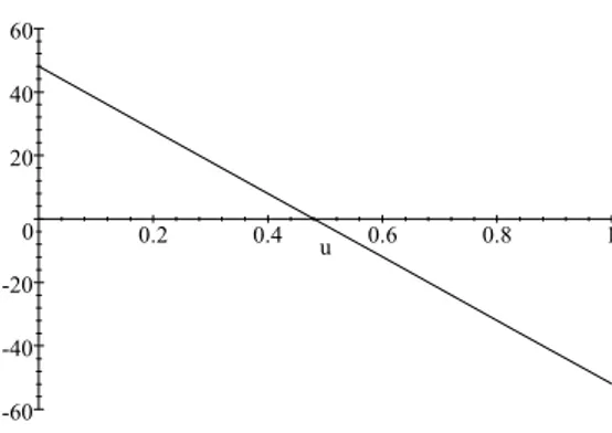
The derivative of exports in relation to local share of …rms is:
dx ds =
N t Á(N+ 1)
¡
2rµ2M¡°(N+ 2)¡µ2M¢¡°2(N+ 1)¢ (34)
We opted again to use simulation methods to check the sign of the derivative. The central case is once again: N = 100,A= 50,L= 50(i.e.: M = 100),t= 2,
µ = 5, ° = 3000, and D = 5000. As it can be seen in the …gure bellow the derivative is only positive for u inferior to a threshold value. For u superior to a threshold value the derivative is negative (the expression is negative for
u >0:70, and the reverse foru <0:70). This comes in contrast with the SCM and MCM. This happens to be so because for higher values ofuthe exporting market becomes to small for allowing exports to increase for home …rms. The RDM therefore captures the e¤ects of the size of the exporting market.
We also check how these results change with di¤erent values. Once again, changing the level of trade costs (t), or the number of …rms (N), does not a¤ect the results.
-4 -2 0 2 4 6 8 10
0.2 0.4 0.6 0.8 1 u
Figure 4: Derivative ofxin relation tos(central case)
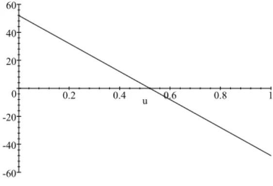
-2 -1 0 1 2 3 4
0.2 0.4 0.6 0.8 1 u
Decreasing ° for 2550, or making L relatively larger than A (for example
A= 10, and L= 90) we get that the threshold value ofudecreases in relation to the central case to values close to one half (see …gure bellow).
-60 -40 -20 0 20 40 60
0.2 0.4 0.6 0.8 1 u
Figure 6: Derivative ofxin relation tos(°= 2550,A= 10andL= 90)
The rational for this is that when°is low, more competitive …rms (i.e.: …rms located in the country with more skilled-labor) …nd it harder to impose their competitive edge over less competitive …rms. Once again lower costs of R&D investment can help less competitive …rms19. And as such less competitive …rms
can compete more e¢ciently with exports of more competitive …rms.
Furthermore if A is relatively larger than L, exports always increase with local share of …rms, since the location patterns of skilled-labor do not a¤ect very much export behavior. If on the contrary L is relatively large to A, location patterns of skilled-labor can a¤ect export behavior, and the derivative is negative foru bigger than a threshold value. This happens because when skilled-labor is very abundant less competitive …rms have more easy access to this factor to compete in more equal terms with more competitive …rms.
4.3.3 Behavior of Outputs: Competitiveness E¤ect
The derivative of local sales and exports in relation to u is the same in both cases:
dq du =
dx du=¡tµ
2L(°(2N(N+2)(1¡s)+1)¡µ2M(2N(1¡s)+1))
Á(N+1) (35)
19This result agrees with those who defend that one of the main roles of industrial policy is
First note, that this derivative is unambiguously positive20. As expected
(but even so not the case under the SCM or MCM), local demand contributes positively for local sales (demand e¤ect). The same is not straight forward in the case of exports. The rational for exports to increase withu is that when
uincreases,kalso increases, and so local …rms become more competitive than foreign …rms. As consequence of this ‘competitiveness e¤ect’, …rms located in the country with more skilled labor can gain market share in the foreign market. Note that this comes in contrast with both the SCM and MCM in whichudid not a¤ect exports and local sales.
This shows the presence of ‘competitiveness e¤ects’ in the RDM. When u
increases in a location this makes …rms in this location to invest more in R&D (‘home market e¤ects’ in R&D). In turn, this makes local …rms more competitive than foreign ones, since they will have lower marginal costs (‘competitiveness e¤ects’) due to R&D investment. Therefore asymmetric labor markets turn …rms asymmetric through the R&D channel leading to ‘home market e¤ects’ in R&D and ‘competitiveness e¤ects’.
4.3.4 Behavior of Prices: Spatial Price Discrimination E¤ect
The derivative of prices in relation to home share of skilled-labor is:
dP du =¡
µ
s¡1
2
¶
2µ2N tL '(N+ 1)
Prices decrease with local share of skilled-workers for s > 12, increases for
s <12, and are unchanged for a symmetric pattern location of …rms (i.e.: s= 1 2).
When demand is increasing in the small industrial country prices can go up for two reasons. First, because some of this extra demand has to be satis…ed by foreign …rms whose products incur in trade costs. Second, because an increase in demand in this country can mean more monopoly power (and as such higher prices) for existing …rms. The contrary happens in the country that hosts more …rms since an increase in local share of consumers has as side e¤ect an increase in R&D and as such reduction in costs and (in the end) in prices. Demand and labor market spatial patterns, and contrary to what happens in the SCM and MCM, therefore in‡uence directly the behavior of prices and this fact comes in side with the evidence on spatial price discrimination literature.
The behavior of prices in relation to home share of …rms is:
dP ds =¡
N t '(N+ 1)
¡
°(N + 1)¡2µ2M(1¡r)¢
Prices at home decrease when competition at home also increases (compe-tition e¤ect). See proof in appendix. The rational is the same as before for
20To see this note that the multiplicative term is always positive, and the same happens
the SCM and MCM, when more …rms are located in one country, consumers from that location do not have to pay for so many products the extra cost of transport costs. As such, in the RDM we also have in place a mechanism sim-ilar to the ‘price index’ e¤ect present in the MCM and SCM: prices are lower in the countries with more industry, and as such welfare is also higher in these locations.
5
Overlapping Market Condition
The overlapping market condition (OMC) gives the threshold level of market size (or trade costs) that makes trade pro…table for …rms (see Brander, 1981). Bellow this threshold level we are in autarchy: exports are too costly for …rms; above this threshold trade is possible: exports are pro…table.
As showed by Brander (1981), theOMCfrom the side of the foreign …rm is obtained by settingx¤= 0, ats= 1and solving for trade costs or market size21.
Therefore, the OMC states the minimum market size necessary (or maximum trade costs level) for a potential foreign …rm be able to export pro…tably to the home country when home hosts all the …rms. This condition can also be de…ned from the point of view of the home …rm. The correspondent OMC from the side of the home …rm is obtained by settingx= 0at s= 0and then also solve for market size or trade costs. The interpretation is the same as before for the OMC from the side of the foreign …rm. We will see below that under the SCM and MCM this condition is the same for both home and foreign …rms. However, under the RDM that is not the case anymore. This happens because …rms can endogenously become asymmetric as result of R&D investment, and being that so, is also natural that home and foreign …rms have di¤erent levels of market access to international markets (i.e.: they have di¤erent OMC).
5.1
Monopolistic Competition Model
In the MCM, the OMC is the same for both a representative home and foreign …rm. In fact whatever settingx¤= 0ats= 1, orx= 0ats= 0, and then solve for trade costs, the result comes that for all levels of trade costs trade is always possible, sincet >122. Therefore under the MCM trade is never forbidden.
5.2
Standard Cournot Model
In both the SCM and the RDM we opt by de…ning the OM C in relation to market size23. Then by settingx¤= 0, ats= 1and solving for Dwe get:
21Note that in all models considered is possible to solve the OMC for the trade costs variable.
On the contrary it is only possible to solve the OMC for the market size variable in the oligopoly model (since the monopolistic competition model does not have the variable market size).
22Only whent= 0, it is not pro…table for a potential home or foreign …rm to export, but
since iceberg trade costs assumet >1, then trade is always possible under the MCM.
23We opt for de…ne the OMC in relation to market size for two reasons. The …rst one, is
D > t(N+ 1) (36)
As such in the SCM theOM C gives the relation between market size (D) and trade costs (t), and the total number of …rms in the world economy (N), that makes trade pro…table for an individual …rm. Trade is restricted the higher the trade costs and the larger the number of …rms in the world economy. The role of trade costs is self explanatory: higher trade cost makes exports more costly. More …rms means more competition, and therefore less output per …rm, and this in turn less pro…tability of exports.
One further point must be made about the OMC. We need to stress that as we have explained in the introduction to this section, the way we de…ned the OMC above, sees trade from the point of view of the foreign …rm: if home host all the industry, the OMC gives the trigger level of market size that makes exports pro…table for a potential foreign …rm (a similar analysis can be made from the point of view of the home …rm). Bellow this threshold level foreign …rms are not able to export to the home market and therefore the home country in practice is protected from foreign competition (i.e.: autarchy)24. However,
and since the model is symmetric the same condition applies for home …rms to export to the foreign market25. Therefore, for D < t(N+ 1)we are in fact
technically in autarchy.
Since we are concerned we international trade questions we want therefore to prevent cases where trade is forbidden. As such we assume through the paper that the OMC for the SCM is always satis…ed, i.e.: D > t(N+ 1).
Finally, we show some comparative statics in the behavior of theOM C. The important thing to note is that, theOM Cis not a¤ected by changes in the local share of consumers (u):
dOMC du = 0
Firms decision to export is not a¤ected by the size of the consumer or labor markets in the destination country (i.e.: trade is not a¤ected by the exporting market demand conditions). This comes as a not very realistic result, since higher potential demand in a country should make it easier for a foreign …rm to export to that country (i.e.: demand should facilitate trade).
reason, is that we think that the natural way for a exporting …rm to look at the foreign market is to know if the market size in that country is su¢ciently big to compensate for trade costs (or all other type of costs as it comes in the R&D model), and not if trade costs are su¢ciently low to export.
2 4Note however, that the OMC is not an entry condition, if …rms are not able to export they
can always sell in their own market. Also, even if export is pro…table, it does not necessarily mean that …rms can enter the market. For example foreign and local competition can prevent entry. Entry and exit analysis need to consider other type of issues as competition, demand, and in general pro…tability.
5.3
R&D Investment Model
TheOM Cfor the RDM (from the perspective of the foreign …rm) comes (setting as beforex¤ = 0, ats= 1 and solving forD)26:
D¤=t(N+ 1) +N µk¡µk¤(N+ 1) (37)
In the RDM theOMC gives the relation between market size, trade costs, and R&D investment byHandF …rms that makes trade possible. It can also be seen that theOM Cincreases with trade cost, and the level of R&D investment by H …rms, while it decreases with the level of R&D investment by foreign …rms. This comes at no surprise, since the more the home …rms invest in R&D more di¢cult foreign …rms will …nd to export to the home market. Conversely, also the more the foreign …rms invest more easily they will …nd to export to the home market.
However now the OMC from the perspective of the home …rm is not equal to the OMC from the perspective of the foreign …rm (as it happen in the SCM). In fact the OMC from the perspective of the home …rm is:
D= (t(N+ 1) +Nµk¤¡µk(N+ 1))
This increases as before with trade costs and the total number of …rms in the world economy, but now the role of R&D investment by home and foreign …rms is inverted. The OMC from the perspective of the home …rm, increases with foreign R&D investment and decreases with home R&D investment.
We can derive the explicit expressions for both OMC (substituting for k
andk¤). The OMC from the perspective of a potential foreign and home …rm, respectively, are:
D¤ = tµ2M(µ2M(2N+1)(1¡r)¡°(2(N2+1)+5N¡r(2N(N+2)+1)))+°2(N+1)2 °(N+1)(°¡µ2M) (38)
D = t°2(N(N+2)+1)¡°µ2M(°r((2NN+1)((N+2)+1)+(°¡µ2M)N+1))+rµ4M2(2N+1) (39)
Once again we stress that since this paper is concerned with international trade questions, we want to rule out cases where trade is not possible for all …rms. However under the RDM, as we will see bellow, it can happen that trade is not possible for foreign …rms but possible for home …rms (and vice-versa). This happens because home and foreign …rms have di¤erent OMC. Being that so we only rule out cases where both home and foreign …rms can not export, but this not necessarily means that we need to assume that the two OMC of the RDM have to be satis…ed. For example it can happen that only the OMC
26We denote market size by an asterisk to stress that this is the OMC from the side of
from the side of home …rms is satis…ed (while the OMC for foreign …rms is not). Then home …rms can export to the foreign country, but foreign …rms can not. If this is the case we will accept this scenario as valid for our analysis. Therefore we only rule out cases where both OMCs (OMC from the side of home …rms and OMC from the side of foreign …rms) are not satis…ed.
5.3.1 Access to International Markets
If home and foreign …rms have di¤erent OMC, they also can have di¤erent levels of market access. This does not happen in the SCM or MCM where all …rms, under all possible scenarios have the same level of market access since they are symmetric in all aspects. On the contrary in the RDM, …rms from one country can have better access to exports markets, since …rms can become asymmetric due to asymmetric labor markets and R&D investment. We investigate under what conditions some …rms can penetrate more easily foreign markets than their foreign competitors. To do this, …rst note that the di¤erence between the OMC of a representative home …rm and the OMC of a representative foreign …rm is:
DOM C¡DOMC¤ =¡2tµ2M
µ
r¡1
2
¶
°(2N(N+2)+1)¡µ2M(2N+1)
°(N+1)(°¡µ2M)
It can be easily check that this di¤erence is negative foru > 12, positive for
u < 12, and zero foru=1227. Then, whenu >1
2, home …rms can penetrate more
easily the foreign market (than their foreign counterparts the home market), since the OMC for home …rms is smaller than the OMC for foreign …rms. The reverse happens foru < 12. This is so because when a country hosts more skilled-labor, …rms located in this country perform more R&D and therefore are more e¢cient and competitive. When this happens …rms from di¤erent countries have di¤erent levels of market access.
Atu= 1
2 the equality for the two OMC observed in the SCM is restored. In
fact atu= 1
2 both OMC are equal and simplify to:
D=D¤= 1 2
³
2°(N+ 1)2¡µ2M(2N+ 1)´ t (N+ 1)°
Therefore, as long as skilled-workers are evenly distributed …rms have the same level of access to international markets. This happens because foru= 12 home and foreign …rms invest the same, and therefore they not become asym-metric. If they are not asymmetric they can not also have di¤erent levels of market access.
The problem comes for u6= 12, since countries are not only made asymmet-ric because of di¤erent labor spatial patterns, but also …rms are asymmetasymmet-ric because they perform di¤erent levels of R&D investment, i.e.: …rms located in
27To see this note that since° > µ2M, then both the nominator and the denominator are
the country that hosts a large share of skilled workers invests more what makes them more competitive. Being that so, more competitive …rms also …nd more easily to penetrate foreign markets than their counterparts.
Given this, we are interested in four issues related with the OMC of the RDM. The …rst thing, is to sign the OMC (i.e.: under what conditions is positive or negative). If it is negative, then we know that it is always satis…ed since
D >0. If on the contrary it is positive, for trade to be possible …rms depend on market size to be able to export. The second issue, relates with how the OMC is related with demand and labor market patterns. More demand in a country makes it easier for …rms to export to that market, or the contrary happens because of labor market e¤ects? This last case can result, because …rms located in countries more endowed in skilled labor are more competitive. The third issue, concerns with how the OMC is related with the OMC of the SCM, i.e.: under what model trade is more restricted (or promoted). Finally, we want to know if the OMC is a su¢ciently condition for the R&D condition (i.e.: condition that assures that R&D investment levels are positive) be satis…ed.
5.3.2 Sign of the OMC: R&D as an Barrier to Trade
It is not a simple task to sign the OMC expression 28. We have chosen to use
simulations to see how this change with di¤erent parameter and variable values. We start by settingµ = 5, M = 100, ° = 3000 (remember that we need that
° > µ2M), t= 2, andN = 100 (see …gure bellow29). For these values we get
that the OMC is negative foru <0:30, and positive foru >0:30. This means that for u < 0:30, trade is always possible for a potential foreign …rm, since
D >0.
The …gure also illustrates the role of market size in international market access. For high values of market size, as it is expected (and as is the case in the SCM), trade is always possible since the OMC is satis…ed. For lower levels of market size (and contrary to the SCM), trade is not possible only for higher values ofu(i.e.: when home hosts relatively more skilled-labor), for lower values of u foreign …rms can penetrate the home market since the OMC is negative andDis always positive. Under the SCM for lower levels of market size trade is never pro…table.
We also check the robustness of the results. The …rst thing to note from this analysis is that changing the level of trade costs (t), or the number of …rms (N) does not change the threshold value ofu. In fact, for example, for N = 10, or
t= 1, we have a similar picture30:
The same forN = 1000,t= 50, we have31:
28We check the sign of the OMC from the perspective of a representative foreign …rm,
but note that the same results apply by symmetry to the OMC from the perspective of a representative home …rm.
29The red line shows the OMC from the side of a representative foreign …rm. The blue line
shows the OMC from the side of a representative home …rm.
30This …gure is plot fort= 1, but a similar picture is obtained forN= 10.
-400 -200 0 200 400 600 800
0.2 0.4 0.6 0.8 1 u
Figure 7: OMC: central case
-200 -100 0 100 200 300 400
0.2 0.4 0.6 0.8 1 u
-10000 -5000 0 5000 10000 15000 20000
0.2 0.4 0.6 0.8 1 u
Figure 9: OMC:N = 1000,t= 50
The only di¤erence in relation to the central case is that the maximum value of market size needed for trade to be always possible is bigger whent orN are larger, and small when t or N are smaller. Therefore when trade costs are smaller and competition softer, trade is made easier.
On the contrary changes in °, µ, M, or in the relation between A and L
a¤ects the threshold value of u. Note then that increasing ° is the same as decreasing µ, or M, and decreasing ° is the same as increasingµ, or M, since these are connected through the stability condition° > µ2M. Increasing °for 5000 (keeping constant the rest of the parameters) we get that the OMC is positive for any value ofu. Then trade to be possible (or not) will depend on whatever market size is su¢ciently high (or not) to make trade possible (see …gure).
-100 0 100 200 300 400
0.2 0.4 0.6 0.8 1 u
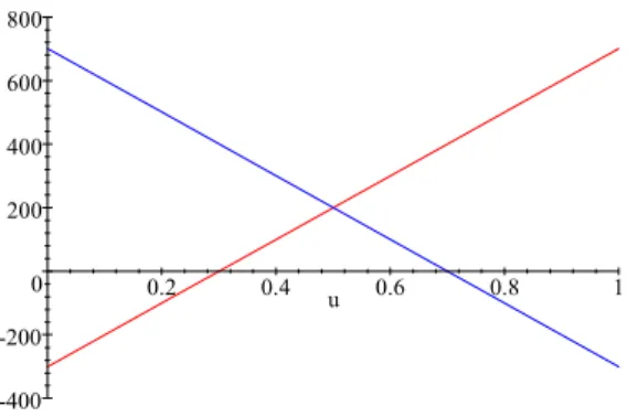
Decreasing ° for 2550 we get that the OMC is negative for u <0:48, and positive foru >0:48(see …gure)32.
-6000 -4000 -2000 0 2000 4000 6000
0.2 0.4 0.6 0.8 1 u
Figure 11: OMC:°= 2550
Then, we have that for very high° in relation toµ2M, the OMC is always positive. Therefore, when this is the case we always need market size to be su¢ciently big for trade to be possible. For lower levels of ° (in relation to
µ2M), the OMC is positive forusuperior to a threshold value ofu, and negative for the reverse. This threshold level ofuhas its maximum at ° close to µ2M
(where the threshold is one-half), and the minimumu= 0 for very high°. As corollary, …rms in the country with more skilled-workers are more pro-tected from foreign competition. This happens to be so because …rms in this country invest more in R&D, as such R&D investment protects …rms from for-eign competitors and its role is similar to trade costs and trade barriers since it prevents foreign …rms to enter the local market through exports. Note however that the maximum value of market size need for trade to be pro…table is lower when° is bigger. This means that higher costs of R&D gives less competitive advantage to …rms from countries that host a higher share of skilled-labor.
Changing the relation betweenAandL(but keeping constantM =A+L), also a¤ects the results. If A is relatively larger in relation to L (for example ifA = 90, and L = 10) then the derivative is positive for any value of u(see …gure).
IfLis relatively larger in relation toA(for example ifA= 10, andL= 90), the OMC is positive foru >0:40, and the negative foru <0:40.
However, the maximum value of market size need for trade to be possible is smaller when unskilled-labor is relatively more than skilled-labor. This happens to be so because when unskilled-labor is relatively more than the skilled-labor …rms …nd it di¢cult to gain competitive advantage over foreign …rms even when the country where they are located host more skilled-labor.
32At°= 2501the OMC is positive foru >0:5 and negative foru <0:5. Therefore the
-100 0 100 200 300 400
0.2 0.4 0.6 0.8 1 u
Figure 12: OMC:A= 90, L= 10
-1000 -500 0 500 1000
0.2 0.4 0.6 0.8 1 u
Figure 13: OMC:A= 10, L= 90
Then the OMC (from the side of a representative foreign …rm) increases with
L, N, t, andµ; and decreases withA and°33. When the world endowment of skilled-labor is big, this will allow more …rms to coexist (whatever the spatial distribution of this factor) and therefore make markets more competitive and exports less pro…table. WhenN is big the same e¤ect occurs, more competition and as such trade more di¢cult for …rms. Also when R&D is very e¤ective (i.e.: high µ), competition will be …ercer and exports more penalized. On the contrary when°is high, competition will be softer because less …rms can stay in the market when the costs of R&D (i.e.: the …xed costs) are larger. WhenAis relatively larger thanL, trade is made easier because there is less skilled-labor to make …rms asymmetric and as such competition harder. Therefore trade is
33We have shown this by simulation methods, but the same result can be obtained by
both related with competition and R&D investment patterns.
5.3.3 OMC and u: Spatial Labor Markets as a Barrier to Trade
Other important thing, is that now, and contrary to the SCM, the OM C de-pends on the share of consumers in a location. In fact the derivative of the OMC in relation touis:
dOM C du =¡tµ
2L°(2N(N+ 2) + 1)¡µ2M(2N+ 1)
°(N+ 1)¡°¡µ2M¢
The derivative of the OMC in relation to the local share of consumers is negative (i.e.: increasingumakes trade more di¢cult for foreign …rms)34. This
is so because when home host a large share of skilled-workers, home …rms also invest more in R&D than their foreign counterparts, and as such home …rms are more competitive than foreign …rms. Therefore, foreign …rms …nd it hard to penetrate the home market both because of trade costs and because home …rms have a competitive edge over them. The contrary happens with home …rms, higher levels ofumake it more easy for them to penetrate the foreign market.
In fact, since the two OMC of the RDM are symmetric (see also …gures above), while the OMC from the side of foreign …rms increase withu, the OMC from the side of home …rms decrease withu. Then it can happen that for high values of u trade is not possible for foreign …rms but it is possible for home …rms (and the reverse for low values ofu). These cases are not possible under the SCM (or MCM) but are important since these can lead to di¤erent trade patterns not present in the SCM or MCM, as we will see bellow.
5.3.4 OMC RDM versus OMC SCM: R&D, Trade and E¢ciency35
As shown in appendix the OMC for the RDM (from the side of the foreign …rm, and by symmetry for the OMC form the side of the home …rm) is superior to the OMC of the SCM foru > 12, and the reverse foru < 12. Therefore, when the home country hosts a larger share of skilled-workers, trade for foreign …rms is restricted relatively to the SCM case. On the contrary, when home hosts less skilled-workers, then foreign …rms will …nd it easier to export to the home market under the RDM case than under the SCM case. Then, we conclude that R&D investment is an impediment for trade for …rms that are not so competitive, but promotes trade for …rms that are more e¢cient, i.e.: there is a close link between R&D, trade and e¢ciency.
34To see this note that the multiplicative term is always positive, and the same for what is
inside parenthesis (since° > µ2M).
35Note that both the SCM and the RDM, are more restricted to trade than the MCM. In
5.3.5 OMC RDM versus R&D condition: Trade as Promoter of R&D
We subtract the OMC (from the side of a foreign …rm) to the R&D condition form the side of a representative home …rm (equation 21), since we want to see the relation between the access of foreign …rms to the home market and the level of R&D performed by home …rms.
This di¤erence depend on both s and u, but the analysis shows that u
determines this relation. To prove this we use again simulation methods, but complement this with graphical analysis. We start by settingµ= 5,M = 100,
°= 3000,t= 2, andN = 100. Plotting the …nal result we get:
0 0.2 0.4 0.6 0.8 1
u 0
0.2 0.4
0.6 0.8
1 s
Figure 14: OMC versus R&D condition: central case
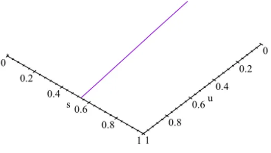
This is positive for the left of the isoline, and negative to the right. Then for u bigger than a threshold level the OMC is always superior to the R&D condition, and the reverse forusmaller than the threshold level. This threshold value changes however withs.
0 0.2 0.4 0.6 0.8 1
u 0
0.2 0.4
0.6 0.8
1 s
Figure 15: OMC versus R&D condition: °= 2550
Changing the relation betweenAandL(but keeping constantM =A+L), also a¤ects the results. IfAis relatively larger in relation toL (for example if
A = 90, and L = 10) then the derivative is positive for most of the values of
u, except for uand svery close to zero. IfL is relatively larger in relation to
A(for example ifA= 10, andL= 90), the threshold value increases from the central case.
Therefore, for most cases if the OMC is satis…ed so it is the R&D condition, i.e.: trade promotes R&D investment. For other cases, …rms to have positive levels of R&D investment will depend on the market size. Note that this problem only arises for …rms in the country with less skilled-workers. The country that hosts a larger share of …rms will always have positive levels of R&D investment. This also indicates that …rms in the market with less skilled-workers have more di¢culties to compete in the world market (and therefore exit of …rms can be promoted). Also, when the HTS is small in the world economy (due for example to a low share of skilled-labor in the world labor markets), then …rms in the HTS will …nd more easy to perform positive levels of R&D investment as long as trade is possible.
6
Patterns of Trade
In this section we try to look at the patterns of trade implied by the MCM, SCM and the RDM. To do this we follow Head et al. (2000) de…ning the Balance of Trade for the home country as:
B=MN((1¡r)sx¡r(1¡s)x¤) (40)