Effect of Horizontal Magnetic Field and Horizontal Rotation on Thermosolutal Stability of a Dusty Couple-Stress Fluid through a Porous Medium: a Brinkman Model

(1)

J_{ournal of}A_ppliedF_luidM_{echanics, Vol. 10, No. 2, pp. 681-692, 2017.} Available online at www.jafmonline.net, ISSN 1735-3572, EISSN 1735-3645. DOI: 10.18869/acadpub.jafm.73.238.27027

Effect of Horizontal Magnetic Field and Horizontal

Rotation on Thermosolutal Stability of a Dusty

Couple-Stress Fluid through a Porous

Medium: a Brinkman Model

K. Kumar

1†

, V. Singh

2

and S. Sharma

1

1_{Department of Mathematics and Statistics, Gurukula Kangri Vishwavidyalaya, Haridwar, 249404, India.} 2_{Department of Applied Sciences, Moradabad Institute of Technology, Moradabad, 244001, India.}

†Corresponding Author Email: kkchaudhary000@gmail.com (Received August 5, 2016; accepted November 27, 2016)

A

BSTRACT

The problem of the onset of double diffusive convection in a couple-stress fluid saturated with a porous medium is studied under the effects of magnetic field, rotation and suspended dust particles. Linear stability analysis based on the method of perturbations of infinitesimal amplitude is performed using the normal mode technique for the case of free-free boundaries. The governing hydrodynamic and hydromagnetic equations of fluid flow are governed by the Brinkman model. The stability analysis examines the effects of various embedded parameters for the stationary mode both analytically and graphically. The principle of exchange of stabilities holds good in the absence of solute gradient parameter. Also, the sufficient conditions responsible for the existence or non-existence of overstability are obtained.

Keywords: Couple-stress fluid; Magnetic field; Rotation; Dust particles; Brinkman porous medium.

N

OMENCLATURE

t

time

coordinate,

d

thickness of porous fluid layer,

q

fluid velocity vector having

components

d

q

suspended particle velocity having

components

p

pressure

0

T

reference temperature

0

S

reference concentration

T

temperature

S

concentration

K

stokes’ drag coefficient

0

N

number density of dust particles

1

k

Darcy-brinkman medium permeability

T

k

coefficient of heat conduction

S

k

coefficient of solute concentration

D

differential operator

m

mass of suspended particles

n

frequency of the harmonic disturbance

i

X

gravitational acceleration vector

s

c

heat capacity of solid material

v

c

specific heat of the fluid at constant

volume

w

vertical fluid velocity

s

vertical particle velocity

*

w

_{complex conjugate of}

H

horizontal

magnetic

field

having

components

h

perturbation in magnetic field

strength

X

vertical

component

of

current

density after applying normal mode

method

W

vertical component of fluid velocity

after applying normal mode method

K

vertical component of magnetic

field after applying normal mode

method

Z

vertical component of vorticity after

applying normal mode method

x

k

wave number in x direction

y

k

wave number in y direction

(2)

p



pressure gradient term

0



density of fluid

s



density of solid material



fluid

viscosity



couple-stress fluid viscosity

ef



effective

viscosity

ef



effective kinematic viscosity

e



magnetic

permeability

T



thermal expansion coefficient

S



solute expansion coefficient

T



adverse temperature gradient

S



solute concentration gradient



electrical resistivity

Θ

temperature component after applying

normal mode method



solute component after applying

normal mode method

p



perturbation in fluid pressure p



perturbation in fluid density





kinematic

viscosity



kinematic

viscoelasticity

T



thermal

diffusivity

S



solute

diffusivity



z-component of vorticity



z-component of current density

Ω

horizontal

rotational

vector

having

components

2



3-dimensional Laplacian operator



growth rate of harmonic disturbance

after applying normal mode method



perturbation in temperature T



perturbation

in

solute

concentration

S



Suspended particles radius

i



vertical unit vector

Non-dimensional Parameters

a

dimensionless wave number

l

P

dimensionless medium permeability

1

p

thermal Prandtl number

2

p

magnetic Prandtl number

1

q

Schmidt number

B

suspended particle parameter

1

Q

modified Chandrasekhar’s number

1

A

D

modified Darcy-Brinkman number

1

R

modified

Darcy-brinkman

thermal

Rayleigh number

1

S

modified solute Rayleigh number

1

A

T

modified Taylor’s number



Darcy-Brinkman medium porosity

1



modified couple-stress parameter

1. I

NTRODUCTION

The study of fluid dynamics is of great importance for scientific researchers and engineers to understand various significant and fascinating applications of fluid mechanical phenomena such as calculating forces and moments on aircrafts, determining the rate of mass flow in oil industry through pipelines, forecasting weather patterns, understanding nebulae in interstellar space and in traffic engineering by considering traffic as a continuously distributed fluid. Copious literatures (Lin, 1955; Batchelor 1967; Rajagopal, 1978; Drazin and Reid, 1981; Bansal, 2004; Gupta and Gupta, 2013) are available that provide a basic theoretical and experimental support for various fluid dynamical phenomena as well as hydrodynamic stability of Newtonian and non-Newtonian fluids. The influence of magnetic field and rotation on thermal instability of an incompressible Newtonian fluid layer has been the subject matter of great interest over the years since the pioneering work by Chandrasekhar (1981) within the framework of linear stability theory. In double diffusive (when the fluid layer is simultaneously heated and soluted from underside) phenomena, convection process is induced by the combined effects of temperature difference and concentration difference which have different diffusion rates. Double diffusive (thermosolutal) convective phenomena through a porous medium frequently

occur in seawater flow, mantle flow in earth’s crust, ground water hydrology (underground disposal of nuclear wastes), astrophysics (helium acts like a salt in raising the density in stellar case), oceanography, soil science (transportation of soil, solid waste and mud particles into the rivers and lakes), solar system (where heat and helium diffuse at differing rates), atmospheric science and limnology.

(3)

683 of rotating fluids which has applications in various technological situations which are governed by the action of coriolis force. The double diffusive convective problems of couple-stress fluid through an anisotropic porous medium considering rotational effect have been discussed in the references by Malashetty and Kollur (2011) and Malashetty et al. (2011). A major part of the universe is filled with charged particles and magnetic field is present in and around the heavenly bodies. Magnetic field plays a dominant role in several clinical purposes such as in neurology and orthopaedics for examining the internal organs of the body in various diseases like tumours detection, heart and brain diseases, stroke damage etc. The theory of magneto-hydrodynamics (MHD) has several scientific and practical applications in geophysics (in the study of earth’s core), atmospheric science (solar wind is governed by MHD), astrophysics, plasma physics, space sciences etc. Thermal instability problem of an electrically conducting couple-stress fluid heated from below through a porous medium in the presence of a uniform magnetic field has been investigated by Sharma and Thakur (2000). Sharma and Sharma (2004) have considered the effect of suspended particles on couple-stress fluid heated from below in the presence of vertical rotation and vertical magnetic field and noted that the effect of rotation is to stabilize the system, whereas suspended particles have destabilizing effects. Thermosolutal convective problem for a couple-stress fluid through a porous medium under the influences of uniform vertical magnetic field and uniform rotation has been studied by Singh and Kumar (2011), whereas the effect of suspended particles on couple-stress fluid heated and soluted from below through a porous layer has been noted by Sunil et al. (2004).

Couple-stress theory due to Stokes (1966) is of vital importance to understand different aspects including the lubrication mechanism and functioning of synovial joints during human locomotion and opened new vistas in several areas of scientific and technical research. Shivakumara et al. (2011) illustrated the linear and nonlinear stability problem of double diffusive convective phenomena for couple-stress fluid through a porous layer. Kumar et al. (2015a, b, 2016) considered, theoretically, thermal convection problems for both couple-stress fluid and ferrofluid to include the effects due to magnetic field, rotation, compressibility, variable gravity and heat source strength through Darcy as well as Brinkman porous medium. Thermal as well as thermosolutal convective instability problems through a porous medium have extensive attention over the years and also recognized as the problems of fundamental importance in solidification and chemical processing industry, bio-medical sciences, geophysical fluid dynamics, soil sciences, petroleum industry and filtering technology. Extensive reviews related to thermal and thermosolutal convective problems through a porous medium have been covered in the books by Ingham and Pop (2005), Vafai (2000, 2005), Nield and Bejan (2006) and Vadasz (2008). McDonnel (1978) has conducted extensive and systematic studies regarding the impact of porosity in astrophysical situations because a greater part of

the universe is filled with fine dust particles. It is well known that the Darcy equation fails to give satisfactory results for high permeability porous medium. So, the consideration of non-Darcy (Brinkman) model, which take care of boundary and inertia effects, is of practical interest for high permeability porous medium. Kuznetsov and Nield (2010) analyzed the thermal instability problem in a porous layer saturated by a nanofluid employing the Brinkman model for the porous medium. Mahajan and Sharma (2012) studied the asymptotic stability and also determine the stability bounds for both equilibrium and arbitrary flows of a couple-stress fluid in a Brinkman flow. Recently, the linear and nonlinear stability analysis of double-diffusive reaction convection in an anisotropic Darcy-Brinkman porous layer is performed by Gaikwad and Dhanraj (2016).

Therefore, the Brinkman model, which is physically more realistic than the other ones, is considered for the porous medium to include effects due to horizontal magnetic field and horizontal rotation in a dusty couple-stress double-diffusive convection. Some previous published works by Sharma and Thakur (2000), Sharma and Sharma (2004), Sunil et al. (2004) and Singh and Kumar (2011) can be recovered from the present investigation.

2. M

ATHEMATICAL

F

ORMULATION

Consider an infinite, horizontal porous layer of

thickness

d

of an incompressible couple-stress

fluid with dust particles heated and soluted

from below through a porous medium of

porosity



and permeability

k

₁

. The fluid

layer is acted upon by a uniform horizontal

magnetic field

H



H,0,0



and a uniform

horizontal rotation

Ω 



,0,0



. The fluid layer

is heated and soluted from below such that an

adverse temperature gradient

_T dT

dz 

 



 

 

and

concentration gradient

_S dS dz 

 _ 

 

 

are

maintained. The coriolis effect has been taken

into account by including the coriolis force

term

2



q×



in the momentum equation,

whereas the Centrifugal force term

2

1 grad

2 r

_ _ 

 

 × 

can be realized as a gradient

of a scalar and, therefore, has been absorbed

into the pressure term

1 2

2

f

p_p   r _

 × 

.

The term

p_f

stands for the fluid pressure and



_{denotes the angular velocity of rotation.}

(4)

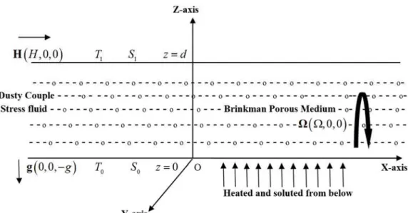
Fig. a. Geometrical Sketch of the Physical Problem.

is extended infinitely in

x

and

y

directions

and the

z

axis is taken vertically upward with

the origin at the lower boundary. The pressure

p

, density



, viscosity



and viscoelasticity



depend upon the vertical co-ordinate

z

-

only.

The basic equations in a double diffusive

convection for an

incompressible couple-stress fluid saturating a Brinkman (1947a, b) porous medium under Boussinesq approximation are defined as

The density equation of state is given by









0 1 T T0 T S S S0

 _     _

(1) Equations of momentum and mass conservation are defined as

 

















2 0

1 2

0 0 0

1 2

1 .

4

ef e

p

k

K N t

  

  

 

_{ } _ _{ }_ _ 

 

  

  

 _ _ _ _ _ _{ }

   

 

          

 

   

 

 

i

d

X q

q

q q q Ω q

q q H H



(2)

. 0

 q (3) Neglecting the variations in pressure force, Darcian force, magnetic field and buoyancy force (due to gravity) on the particles, the equations of motion and continuity for the particles are as









0 0

1 .

mN K N

t 

 _ _ _ _ _

 _ _ 

 

d

d d d

q

q q q q

(4)





0 0

. 0

N N t 

   

 qd (5)

Assuming that the suspended particles and the fluid particles are in thermal and solute equilibrium, the equations for temperature and solute concentration can be presented as





 





0 0

2 0

1 .

.

v s s v

pt T

T

c c c T

t

mN c T k T

t

   

      

 _{ }



 

 _   _  



 d 

q

(6)













0 0

2 0

1 .

.

v s s v

pt S

S

c c c S

t

m N c S k S

t

      

      

 _{ }



 



 _   _  



 d 

q q

(7)

where, ,c c c_v  _s, _pt andk_S denote the analogous solute coefficients.

The Maxwell’s (1866) electromagnetic equations yield





2

t 



      

 H

q H H (8)

and  .H 0 (9)

3. P

ERTURBATION

T

ECHNIQUE

A

ND LINEAR

S

TABILITY

A

NALYSIS

Here, the stability of the basic state of system has been examined by using the perturbation technique. Let the perturbations in the basic variables such as fluid velocity q



0,0,0



, particle velocity



0,0,0



d

(5)

685 be denoted by q u v w



, ,



, qd



l r s, ,



,  , p,  , N ,h h



_x,h_y,h_z



, respectively.

After linearizing the system of Eqs. (1) – (9) and following Boussinesq approximation, the perturbation equations obtained after eliminating the pressure gradient term are as follows



T S



0

       (10)

 



 

2 2 2 2

4 2 2 0 0 0

2 2 2

1 2 1 4 1 1 T S ef e

x y x y

x t _mN m t K t x k                      _  _  _  _              _  _ _ _       ____ _{ } _ _    _ _{ }_ _  _{ }    __ __ _      _ _ _  _     __ _ __ ___   _ _ _{ }_ _ _     z g ζ _w w H w h w                      (11)

 





2 0 0 2 0 1 2 1 1 1 4 ef e x m N m t t K t x k    _{ }     _{ }  _ _ _ _  _{ }_  _{ } _ _    _ _  _ _       __  _ _   _ _    _    __ __ _ __  _           __ _    _           w ζ ζ ζ H ξ ζ  (12)

 

2

t x 

      _ _ _ _         z z h w

H h (13)

 

2

t x 

      _ _ _ _         ξ ζ H ξ (14)





2





T T

E b b

t   



 _{ } _ _  _ _

 _ 

  w s (15)





2





S S

E b b

t   



 __{ }_ _ _  _ _ _

 _ 

  w s (16)

where,









0 0

1 s s , 1 s s ,

v v c c E E c c       _               _      0 0 0 0 and . pt pt v v

m N c m N c

b b c c      _      _     

Differential Eqs. (11) – (16) can be solved using the method of normal modes. Suppose that the perturbations in various physical quantities have a solution with a dependence on x, y and t of the form





     

_{     }





, ,

, , , , ,

, , ,

ex p _x _y

z z ik x ik y n t

             z

W z Z z

w ζ h ξ

K z X z

(17)

Using expression (17), the Eq. (11) – (16) into non-dimensional form reduce to (after dropping the asterisk for convenience)





















 





 

2 2 2 2

1

2 2 4

2 2 2 2 2 0 1 1 1 1 2 0 4 A l l x T S e x f D

D a D a

P P

ga d ik d

D a z z

ik d D a             _ _ _{ } _ _ _  _ _  _            _     _     Ω W z H

Z z K z

(18)

















 

2 2 2 2

1 2 2 0 1 1 1 1 2 4 A l l e x x f D

D a D a

P P ik d ik d          _ _ _{ } _ _ _  _ _  _             H Ω

Z z W z X z

) 9 (1



2 2



 

2

 

2 x

ik d

p D a

    _ _ _ _{ } _       _ _ H

K z W z (20)



2 2



 

2

 

2 x

ik d

p D a

    _ _ _ _{ } _       _ _ H

X z Z z

(21)



2 2



 

2 1

 

1 1 1 1 T T d B

D a p E z   

  

   

 _ _ _ _ _ _

   

  _ __  _W z (22)



2 2



 

2 1

 

1 2 1 1 S S d B

D a q E z   

  

   

 _ _ _ _ _ _

   

  _ __  _W z

(23)

where, the following non-dimensional quantities with the scaling have been used in Eqs. (18) – (23)

2 1

1 2

0

1 2 1 2 0

1 2 ₂

, , , , ,

, , , , , 1 ,

, , , . l T S ef l A

z a nd k

z k P p

d d d

f m

q p N B b

K m

d

P

E E b E E b D

d        _  _       _  _  _ _ _                              _{ }    

The boundary conditions appropriate for the case of two free boundaries are defined as

2 ₀_and_1.

on a perfect conducting bounda 0,

0, ry

W D W X D t

DX K

z

Z a  

        



  _

(24) Eliminating 

       

z , z , Z z ,X z andK z

 

from Eqs. (18)–(23) and considering an appropriate solution for W (vertical component of fluid velocity) of the form

0sin ,

W W l z

(25) a dispersion relation is obtained as follows

















1

2 2

2 3 4 2 1

1 2 3 4 ₂

2 1 1 4 1

2 1 2 3

4 1 2 1 3

cos 1 1 cos 1 cos 0 A

T A A A x _{B i}

A A A A x

i A A Q x

Q A A x x xA S A R A

(6)

where,

























1

2 2 2

2

1 _{4 4} _{2 2} 1 _{2 2} _{2 2} ₂

1 2

1 _{2 2} _{2 2} _{4 4} 1 _{2 2} 1 _{2 2}

2 1 1 1

2 2 1

1 1

2 1

3 1

, , , , ,

, cos , 1 ,

1

1 1 1 1 ,

1 1

l A A A

A x

A

R a P l x

R x i P k

l l l l d

Q T S

l l l l l

D

D k k A x i p E

l

D

i f

A x x

i P P

A x i

 



   

 

    

 

 

  

    



    

    _ _

 _ _ 

_ _     _  

 

   

 

  _ q E_{1 2}_, A₄  _



1 x



i_{1 2}p_, 4

T T T

g d

R  



 (Darcy-Brinkman thermal Rayleigh number)

4 S S

S

g d

S  



 (Solute Rayleigh number)

2 4 2 4 A

d T



 Ω (Taylor’s number)

2 2 0 4

e d

Q 

 

 H (Chandrasekhar’s number)

Equation (26) is the required dispersion relation accounting the effects of suspended particles, horizontal magnetic field, horizontal rotation, medium permeability and medium porosity on thermosolutal instability of a couple-stress fluid saturating a Brinkman porous medium.

4. T

HE

S

TATIONARY

S

TATE

In a stationary convection, the marginal state occurs when  0(i.e. growth rate vanishes). Substituting

0

  in Eq. (26), the stationary Rayleigh number 1

R in terms of various parameters and the square of wave number

x

is obtained as





_

_













_

_

1

2 2

1 1

2 2

2

1 1

1 1 cos

1 1

1

1 cos 1

1 1 cos

A

A A

D

x Q x x

x P

R S xB

Bx

T x x

D x

x Q x

P



 

 

       

   _ _ _   _ 

     

 

 _ _

 



_ 

 _ _ _ _ _ _

   

 __ __{  }_ _ _ __ _

 _ _ _ _ _ _ _

 

 

(27) The effect of various parameters on thermosolutal convection can be realized analytically by evaluating the following derivatives

1

1 1 1 1

1

, , , ,

A

dR dR dR dR dT dS d dB .

1

1 1 1 1

1 1

, , and

A

dR dR dR dR

dQ d dD dP

Equation (27) yields













1

2 2

1

2 1

1 cos

A

x P dR

dT _B _{x G} _{Q Px}

 

 _ 

 

  _{  } _ 

 

 

(28)

1 1

1 dR dS 

(29)





























1

2 1

2 2 2

1 1

2 1 1

1 cos

1

1 cos

A

T P x G

Q

x G Q Px x

dR

d B _{T P} _x

x G Q Px

 



 _ 

 _ 

 _{ } _ 

 _ _

  _ _

  _ _ _



 _{  } _ 

 

 

(30)















1



2 2

1

1 2 2

2

2 1

1 1 cos

1

1 cos

1

cos A

x G Q x x

P dR

T x x

dB B x

x G Q x P



 _ _ 

  



 

  _  _



 _{ } _

   

 _ _

 

(31)















1



2 2

2 1

2 2 1

1 1 cos 1 cos

1

1 cos

A T P x x x

dR

dQ B

x G Q Px

 



 



  

 _  _

 _ _{ } _ _

 

(32)















1



2 2

3 1

2 2 1

1

1 cos 1

1

1 cos

A

T P x x

x dR

d BPx

x G Q Px

 

 



  

 _  _

 _ _{ } _ _

 

(33)















1



1

2 2

3 1

2 2 1 1 cos 1

1

1 cos

A A

T P x x

x dR

dD BP x _{x G} _{Q Px}

 

 



  

 _  _

 _    _

(34)















1



2 2

1

2 2

2 1

1 cos

1 1

1 cos

A

T x x G

x G

dR

dP Bx _{x G Q Px} P

 

 



  

 _  _

   

 

(35)

where, 1





1

1 DA 1 .

G    _ _ _ x 

   

 

From the derivatives (28) - (35), it is clear that the Taylor’s number and solute gradient rule out the possibility of the onset of convection, whereas suspended particles and medium porosity accelerate the onset of convection. The magnetic field, couple-stress and Darcy-Brinkman parameter have stabilizing (or destabilizing) effect and the medium permeability has a destabilizing (or stabilizing) on thermosolutal instability if





₂ 2





₁ ₂





₂

1

1 x G Q Pxcos or T P x_A 1 x cos 

      

 

respectively. In the absence of rotation



i e T. . A10



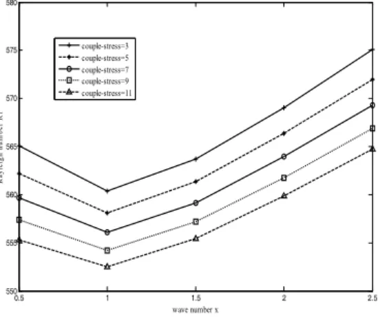
, magnetic field, couple-stress and

(7)

687 state against various values of parameters such as rotation, solute gradient, medium porosity, suspended particles, magnetic field, couple-stress, Brinkman number and medium permeability on double-diffusive convection saturating a Brinkman porous medium are depicted graphically in Figs. 1-8, respectively for45 .

Fig. 1. Variations of

R₁

with

x

for various

values of rotation parameter





1

A

T 1000, 5000,10000, 20000, 40000

and

1

1 1

5, 200, 2, 3, _A 20, 20,

B S   P D   

1 200, 45 .

Q   

Fig. 2. Variations of R₁ with

x

for various values of solute gradient parameter





1 100, 200, 300, 400, 500

S  and

1 1 1

10, 10, 5, _A 25, 25, 200, B P  D    Q 

1 10,000, 45 .

A

T   

5. P

RINCIPLE

O

F

E

XCHANGE

O

F

S

TABILITIES

Here, the conditions have been derived, if any, under which principle of exchange of stabilities (PES) holds true and also the possibility of oscillatory modes.

Fig. 3.

Variations of R₁ with

x

for various

values of medium porosity



2, 4, 6,8,10



and

1

1 1 1

5, 3, 200, 200, _A 20, 20, B P S  Q  D   

1 4000, 45 .

A

T   

x

for various values of suspended particlesB 5,10,15, 20, 25

and

1 1 1 1

20, 5, _A 25, 25, 500,_A 20,

P  D    Q T 

1

000,S 200,45 .

x

for various values of magnetic field





1 2 0 , 4 0 , 6 0 , 8 0 ,1 0 0

Q  and

1 1 1

10, 2, 20, _A 20, 20, _A 10,

B  P D    T 

1

000,S 500,45 .

0.5 1 1.5 2 2.5

220 240 260 280 300 320

wave number x

R

ayl

ei

g

h

nu

m

b

er

R

1

TA=1000 TA=5000 TA=10000 TA=20000 TA=40000

0.5 1 1.5 2 2.5

100 150 200 250 300 350 400 450 500 550

wave number x

Ra

yl

ei

gh num

be

r R1

S1=100 S1=200 S1=300 S1=400 S1=500

0.5 1 1.5 2 2.5

210 220 230 240 250 260 270 280

wave number x

R

ayl

ei

g

h

nu

m

b

er

R1

porosity=2 porosity=4 porosity=6 porosity=8 porosity=10

0.5 1 1.5 2 2.5

200 205 210 215 220 225 230 235 240 245 250

wave number x

R

ayl

ei

gh num

be

r R1

B=5 B=10 B=15 B=20 B=25

0.5 1 1.5 2 2.5

520 525 530 535 540 545 550 555

wave number x

R

ayl

ei

g

h num

be

r R

1

(8)

Fig. 6. Variations of R₁with

x

for various values of couple-stress parameter₁



3,5,7,9,11



and

1 1 1

5, 5, 15, _A 10, _A 40,000, 500,

B  P D  T  S 

1 100, 45 .

Q   

Fig. 7. Variations of

R1

with

x

for various

values of Darcy-Brinkman parameter





1 4,8,12,16, 20

A

D

and

B  3, 2,P15, 1 5,

1 20,000, 1 500, 1 100, 45 .

A

T  S  Q   

Fig. 8. Variations of

R₁

with

x

for various

values of permeability

P



10, 20,30, 40,50



and

1 1 1

10, 2, A 10, 5, 40, B  D    Q 

1 10,000, 1 500, 45 .

A

T  S   

For this purpose, multiplying Eq. (18) by Wand then integrated over the range of z. Using Eqs. (19)-(23) with the help of boundary conditions (24) gives

























1 1

2 2

1 * 1

3 1 1 4 1

2

* 1

5 1 2 6

1 1

2

7 1

1 1

1

1 1

1

l

A T

l T

S S

A

l l

f

I P

D g a

I

P p

I p E I

B

g a

I q E I

q B

D f

d I

P P



   

  _

 

   _

  



 

 



_   _

__  _ _ 

   

 

    

 

_ _ 



 

 

  



 

 _ 

 

  

 _ _ 



 

        

   

 __  _ _   _ 



   

 









8 2

*

2 9 10 2 11 12

0 2 0 2

0

4 4

e e

I

d

p I I p I I

p p

 

 

 

 

 



  

 

 

    

(36) Substituting,  _ri_i in Eq. (36) and equating real and imaginary parts leads to







 



















































2

1 2

1 7

2 2

1

1 1

2 2 ₂

1 1 1 1 1 4

2 2 2 ₁

1 1

2 2

1 1 1 1 2 6

2 2 2 ₀

1 1

2

9 11

1 1

1 1 1 1

4

r T

T

r i

r r i _S

S

r i

r

r r i _e

r i

f g a

I d I

p

B p E I _g _a

q B

B q E I

B

I d I

  



   

      _



   



      _



   

   



  _  _ _ 

_  

 

 

  



 _ _ _ 

 _{ }

 

_ _ _ _

_ _ 



 _ _ _ 

 _{ } 

 

 

 

 



 _













 





















































2 2 2

1 7 1 1 7

2 2

1 1

2 2 8

1 2 2

1 1 1 3

2

1 1 1 4

2 2 2

1 1

2 2

1 1 1 5

2

1 1 2 6

2 1

1 1

1

1 1

i

l _r _i

A T

l T

r r i

i

r i

r r i

i

r

I d I f I d I

P

D I I g a

P p

B I

B p E I

B

B I

B q E I

B

 

   

 

     

 

   

     

 

            

 

 _  _

  

  

 

 

   

 



 _ _ _ _

 

 _ 

 

  _ _ 

 

 

   

 

 









2 2 1

2 2

12 10

1 0 2

0

4

i

S e

S

g a d

I I

q p

 

 

 

 

 

 _{ }

 

 

  

  

 _ _

  

 



_ _ _ 

 

 

(37)

0.5 1 1.5 2 2.5

550 555 560 565 570 575 580

wave number x

R

ayl

ei

gh

num

be

r R1

couple-stress=3 couple-stress=5 couple-stress=7 couple-stress=9 couple-stress=11

0.5 1 1.5 2 2.5

575 580 585 590 595 600 605 610

wave number x

R

ay

le

igh num

be

r R

1

Brinkman parameter=4 Brinkman parameter=8 Brinkman parameter=12 Brinkman parameter=16 Brinkman parameter=20

0.5 1 1.5 2 2.5

535 540 545 550 555 560

wave number x

R

ay

le

igh num

be

r

R

1

(9)

689 and



  























































2 1 2 2 1 1 1 2 2

1 1 1 1 1 4 1

3 1 1 4

2 2 2

1 1

2 2

1 1 1 1 2 6

2

1 5 1 2 6

2 2 2

1 ₁ ₁

2 1 1 1 1 1 1 1 T T r i

r r i

r

r i

i

r r i

r S

S _r _i

f g a

I p

B p E I B

I p E I B

B q E I

B I q E I g a q _B d                         _{ } _{ }    _  _   _ _ _ _    _ _ _ _ _     _     _ _         _ _ _ _    _ _       _ _        







  









2 9 11 1 7 2 2 0 1 1 0 1 2 1 4 1 e r r i

I d I f I                                 _   _ _         _ _         _ _            _ _{ }      _ _ _ _    _ _ _ _    _ _ _ _   (38) where, the positive defined integrals I₁I₁₂ are defined below as









 





 









 

1 2 2 2

1 ₀ 2

1 2 4 2 2 2

2 ₀

1 2 2 2 1 2

3 ₀ 4 ₀

1 2 2 2 1 2

5 ₀ 6 ₀

1 2 1 2 2 2

7 ₀ 8 ₀

1 2 2 2

9 ₀

2

1 2 4 2 2 2

10 ₀

1 2 2

11 ₀ 12

, 2 , , , , , , , , 2 , ,

I DW a W dz

I D W a W a DW dz

I D a dz I dz

I Z dz I DZ a Z dz

I DK a K dz

I D K a K a DK dz

I X dz I DX

     _   _                       _   _    



1



2 2



0 a X dz.



Equation (37) implies that either_r 0 or_r0, meaning that the modes of the system may be unstable or stable, respectively. Thus, it is concluded that the modes may be oscillatory or non-oscillatory. Equation (38) implies that



_i may be either zero or zero, which signifies that the modes may be non-oscillatory or non-oscillatory, respectively.

In the absence of solute concentration



i e. ._S 0



, Eq. (38) gives Eq. (39).

As the terms inside the bracket in Eq. (39) are positive. So,



_i0 which assures that the oscillatory modes are not allowed and also confirms the validity of the PES in the absence of solute concentration gradient with the condition thatB1.

Hence, the oscillatory modes are dominant due to the presence of solute concentration gradient



_Sonly.



 







































 











2 1 2 2 1 1 1 2 2

1 1 1 1 1 4 1

3 1 1 4

2 2 2

1 1

2

1 2

7 9 11

2 2 0 1 1 1 1 1 1 1 1 2 1 4 1 T T r i

r r i

r i

r e

r i

f g a

I p

B p E I B

I p E I

B

f d

I I d I

                                 _  _  _        _ _     _ _ _ _ _       _   _ _ _ _    _ _               _ _ _    _ _ _ _      0                  _{ }    _  _  _  _  _  _  _     (39)

6. O

VERSTABILITY

C

ASE

Here, the possibility whether the observed

instability

may actually be overstability has been examined.

Rewriting Eq. (26) in the following form





































































2 † 1

1 1 1 2 1

1 1 2 1 2

† 1

2 1

1 2 1 1 2 1

1 1 1

1 2 2 1 1 1 1 1 1 1 1

1 1 1

1

1 1 1 cos

i f

G x i p E

i

x i q E x i p

i f

G i

x x i p x i q E Q x

x i p E

i f i x  _               _ __ __ _  _ __ __ _ _ _             _ _ _ _     _ _   __  _  _                             _      





















































† 2

1 1 2 1 2

2 2

2 1 2 1

1 1 1

2 1 2 1

1 1 2 1 2 1

† 1

2 1

2

1 1 1 1 2

1 1 cos 1 1 1 1 1 1 1 1 G

x i q E x i p

B i B i

R x Q R x

i i

x i q E x i p S x

i f

G i

x i p E x i p

    _               _   _  _          _ _ _ _           _   _                _ _   __  _  _             





















































2 1 2 1 2 2

1 1 1 1 1 1 2

† 1

2 1 2 1

1 2 1 1 1

2 1

1 1 2

2 2 4

1 2 1

1

cos 1 1

1 1 1 1 1 1 1 cos 1 cos B i i

Q S x x i p E x i p

i f

G i

B i

x i p x i p E i

x i q E

Q x x Q x x

            _ _          _                  __  _  _           _ _ _ _ _    _                      _ _   









































1 2

1 1 1 1 1 2

2

1 1 1 1 1 2 1 2

cos

1 1

1 1 1 0

A T x x i p E x i q E