Março de 2015
Working
Paper
379
Demand expectations and the
timing of stimulus policies
Os artigos dos Textos para Discussão da Escola de Economia de São Paulo da Fundação Getulio
Vargas são de inteira responsabilidade dos autores e não refletem necessariamente a opinião da
FGV-EESP. É permitida a reprodução total ou parcial dos artigos, desde que creditada a fonte.
Demand expectations and the timing of stimulus
policies
∗
Bernardo Guimaraes
†Caio Machado
‡December 2014
Abstract
This paper proposes a simple macroeconomic model with staggered investment de-cisions. The model captures the dynamic coordination problem arising from demand externalities and fixed costs of investment. In times of low economic activity, a firm faces low demand and hence has less incentives for investing, which reinforces firms’ expectations of low demand. In the unique equilibrium of the model, demand expecta-tions are pinned down by fundamentals and history. Owing to the beliefs that arise in equilibrium, there is no special reason for stimulus at times of low economic activity.
JEL Classification: D84, E32, E62
Keywords: Demand expectations, coordination, fiscal stimulus, timing frictions
∗We thank the editor Francesco Caselli, three anonymous referees, Marios Angeletos, Braz Camargo,
Felipe Iachan, Nobuhiro Kiyotaki, V. Filipe Martins-da-Rocha, Stephen Morris, Alison Oliveira, Ana Elisa Pereira, Mauro Rodrigues and Mark Wright as well as seminar participants at U Carlos III, LACEA-LAMES 2014 (Sao Paulo), NASM-ES 2014 (Minneapolis), Princeton, PUC-Rio, Sao Paulo School of Economics – FGV, U Sao Paulo, SBE 2013 (Igua¸cu), the XVII Workshop of International Economics and Finance (San Jose) and U Zurich. Bernardo Guimaraes gratefully acknowledges financial support from CNPq. Caio Machado gratefully acknowledges financial support from CAPES and FAPESP.
1
Introduction
Pessimistic expectations are often said to play a role in recessions. This idea is captured by models with demand externalities that generate strategic complementarities in production.1
In times of low economic activity, a firm faces low demand and thus has low incentives for investment. In a dynamic setting, this feedback effect may trap the economy in a regime of low output. One important policy issue is then the optimal stimulus policy for an economy subject to this dynamic coordination problem. Is there any special reason for stimulus at times of low economic activity owing to this coordination channel?
This paper develops a model that features this dynamic coordination problem. Invest-ment decisions are staggered, hence economic activity is a state variable. A firm’s optimal investment decision depends on its expectations about others’ actions in the future. Natu-rally, the optimal policy also depends on those expectations. The model generates a unique set of rationalizable beliefs about others’ actions. The beliefs that arise in equilibrium ex-actly offset the dynamic coordination problem faced by firms, so there is no special reason for stimulus at times of low economic activity.
The model features monopolistic competition. Investment is a payment of a fixed cost that increases production capacity. Returns to investment depend on future demand, and hence on whether producers with subsequent investment opportunities choose to take them as well. Thus investment decisions are strategic complements. Producers of each variety receive investment opportunities according to a Poison clock, a simple way to capture pro-duction decisions that can not adjust overnight. This assumption implies that investment decisions are not synchronized, so a producer has to form expectations about others’ future decisions when deciding about investment.
Return to investment depends not only on demand but also on productivity. If the increase in production resulting from investing is large enough, then investing is a dominant strategy. Likewise, if productivity is very low, investing is a dominated strategy. In an intermediate range, a producer’s decision depends on his expectations about the actions of others. In a world with no shocks, that gives rise to multiple equilibria. There is a region of parameters where investing is the optimal decision if agents expect others to do so, but refraining from investment is the best choice in case of pessimistic beliefs.
The solution to the planner’s problem in the environment with no shocks differs from the decentralized equilibrium in three ways: (i) there is no room for multiplicity of beliefs, as one would expect; (ii) the planner requires a lower productivity to invest because it internalizes the benefits to consumers from selling at a cheaper price (monopoly distortion); and (iii) the difference between the planner’s solution and the decentralized equilibrium is
particularly large at times of low economic activity.
The third point is particularly important. Agents might get stuck in a situation where economic activity is low, hence there is low demand and firms prefer not to invest even though productivity would be high enough to encourage investment if demand were high. In this situation, firms would like others to invest, so that demand would increase and then they would be happy to invest as well. A dynamic coordination problem means nobody wants to be the first to invest and the economy is trapped in a situation with low economic activity. The planner would be particularly keen to invest in this situation.
Once we allow for shocks, a unique equilibrium arises in the model, as in Frankel and Pauzner (2000). There is no room for arbitrary beliefs, agents’ expectations are pinned down by the model. The basic idea is that fully pessimistic beliefs are not rationalizable in a region where a small shock to productivity would make it dominant for all firms to invest. Likewise, fully optimistic beliefs are not rationalizable in a region where a small shock to productivity takes the economy to a region where investing is a dominated strategy. Agents know all others will reason like this and try to anticipate what others will do. This process yields a unique rationalizable set of strategies and a unique set of beliefs.
The main result of the paper is that owing to the beliefs that arise in equilibrium, the third difference between the planner’s solution and the decentralized equilibrium vanishes. The maximum amount of investment subsidies the planner is willing to provide at times of high and low economic activity is exactly the same. There is no special reason for subsidies at times of low economic activity.
How are equilibrium beliefs? Consider an agent indifferent between investing or not in a state of low economic activity. She understands that if fundamentals get a bit worse, firms will still be refraining from investing but there will be no major change in the state of the economy. Conversely, a slight improvement in fundamentals will trigger a recovery because firms will choose to invest and that will push the economy to a situation where investing is profitable for everyone. Owing to larger demand, firms will then have more incentives to invest, so it will take a large negative productivity shock to offset the benefit from increasing demand and stop the recovery. The fundamental asymmetry is that bad news basically leave the economy parked in a region of inaction, while good news drive the economy to a different state. The recovery is thus just waiting for a small piece of good news. Hence, in a pivotal circumstance, optimistic beliefs make perfect sense at times of low economic activity. The same reasoning implies that in a pivotal circumstance with high economic activity, beliefs will be more pessimistic: the economy is close to an investment slump.
Equilibrium beliefs solve the dynamic coordination problem. The only remaining difference between the planner’s solution and the decentralized equilibrium is the externality due to market power (which is unrelated to economic activity with (standard) constant elasticity specifications for consumption and production).
The demand externalities that play a key role in this paper are in the seminal con-tributions by Blanchard and Kiyotaki (1987), Kiyotaki (1988) and Murphy et al. (1989). When others produce more, the demand for a particular variety shifts to the right, and its producer finds it optimal to increase production. In Kiyotaki (1988), multiple equilibria arise because of increasing returns to scale. The model in this paper would also give rise to multiple equilibria in the absence of shocks to fundamentals or timing frictions, owing to the assumption of a fixed cost that increases production capacity.
A branch of the literature takes expectations to be driven by some “sunspot” variable, or simply, in the words of Keynes, by “animal spirits”. Depending on agents’ expectations, coordination failures might arise and an inefficient equilibrium might be played.2 Despite
generating interesting insights, this approach does not allow us to understand how policies affect expectations. In models with multiple equilibrium, government policies can only hope to eliminate the “bad equilibrium”. Here, in constrast, policies affect agents’ beliefs about others’ actions.
This paper is closely related to the theoretical contributions in Frankel and Pauzner
(2000) andFrankel and Burdzy(2005) that resolve indeterminacy in dynamic models. They study models with time-varying fundamentals and timing frictions similar to the ones em-ployed in this paper, and prove there is a unique rationalizable equilibrium in their models.3
The results in Frankel and Pauzner (2000) guarantee a unique equilibrium in our baseline model and we use the results of Frankel and Burdzy (2005) in one extension of the model.4
This paper is also related to the global games literature, which has been used to study a wide variety of economic problems that exhibit strategic complementarities, but differently from that literature, there is no asymmetric information in this model.5
There has been a lot of research incorporating strategics complementarities and coordi-nation issues in macroeconomics.6 However, there has not been much work applying those
2See, e.g.,Cooper and John(1988),Benhabib and Farmer(1994) andFarmer and Guo(1994).
3Models with time-varying fundamentals and timing frictions have been used to study other dynamic
coordination problems. Frankel and Pauzner (2002) employ a similar structure in order to analyze the timing of neighborhood change. Guimaraes (2006) studies speculative attacks. Levin (2009) studies the persistence of group behavior in a collective reputation model. He and Xiong(2012) study debt runs.
4See alsoBurdzy et al.(2001).
5See the seminal papers byCarlsson and Van Damme(1993) andMorris and Shin(1998). For a detailed survey, seeMorris and Shin(2003).
theoretical insights to understand the effects of stimulus packages on coordination. One important exception is S´akovics and Steiner (2012). They build a model to understand who matters in coordination problems: in a recession, who should benefit from government subsidies? The results point that the government should subsidize sectors that have a large externality on others but that are not much affected by others’ actions. Differently from a large literature that deals with coordination failures and expectations in macroeconomics, our focus is not on noisy and heterogeneous information, fundamentals are common knowl-edge here, all the action comes from dynamic frictions. This makes our framework specially suitable to understand the dynamic interplay between economic activity, productivity and beliefs that arise in equilibrium.
The paper is organized as follows. Section 2 presents the model in its simplest form. Section 3 describes the decentralized equilibrium and Section 4 shows the solution to the planner’s problem. Section5then explains the result, highlighting the role of beliefs. Section
6 deals with important extensions: it shows a more complete macro model that leads to the same results; considers a process for productivity with mean reversion and discusses implementation of the optimal policy. Section7presents some numerical results and Section
8concludes.
2
Model
2.1
Environment
Time is continuous. A composite good is produced by a perfectly competitive representative firm. At time t, Yt units of the composite good are obtained by combining a continuum of
intermediate goods, indexed by i∈[0,1], using the technology:
Yt = ˆ 1
0
y(itθ−1)/θdi
!θ/(θ−1)
, (1)
whereyit is the amount of intermediate goodiused in the production of the composite good
at timet and θ >1 is the elasticity of substitution. The zero-profit condition implies
ˆ 1
0
˜
pityitdi =PtYt, (2)
where Pt is the price of the composite good and ˜pit is the price of good i at timet.
There is a measure-one continuum of agents who discount utility at rate ρ. An agent’s instantaneous utility at time t is given by Ut=Ct, where Ct is her instantaneous
consump-tion of the composite good. The assumpconsump-tion of linear utility implies that policies will be concerned with inefficiencies in production but will not aim at providing insurance to the household.
Agent i ∈ [0,1] produces intermediate good i. Since yit is the quantity produced by
agent i at timet, her budget constraint is given by
PtCt≤p˜ityit≡wiPt.
Prices are flexible and each price ˜pit is optimally set by agent i at every time. Since goods
are non storable, supply must equal demand at any time t.
The assumptions on technology aim at modelling staggered investment decisions in a simple and tractable way. There are 2 production regimes, a High-capacity regime and a
Low-capacity regime. Agents get a chance to switch regimes according to a Poisson process with arrival rateα.7 Once an individual is picked up, he chooses a regime and will be locked
in this regime until he is selected again. Choosing theLow regime is costless. Choosing the
High regime costs ψ units of the composite good.8
An agent in the Low regime can produce up yLt units at zero marginal cost at every
time t, and an agent in theHigh regime can produce up to yHt units at zero marginal cost,
with yHt = AtxH and yLt = AtxL, where xH > xL are constants and At is a time-varying
productivity parameter.9
The High regime can be interpreted as the use of frontier technology, while the regime
Low would correspond to a less productive technology. The cost ψ can be thought of as the cost difference between each technology and the difference yHt −yLt as the resulting
gain in productivity. Agents are locked in a regime until the next opportunity arises. In one interpretation, the equipament will break after some (random) time and the firm will then decide again between a more or less productive technology. Alternatively, that might capture attention frictions.10
7Real world investments require a lot of planning and take time to become publicly known, so investments
from different firms are not syncronized. The Poisson process generates staggered investment decisions in a simple way. As an implication, investment decisions depend on expectations about others’ actions in the near future. For further evidence on non-convex adjustment costs that lead to infrequent investment, see
Hall(2000) andCooper and Haltiwanger (2006).
8Investment is thus a binary decision. As shown inGourio and Kashyap(2007), the extensive margin accounts for most of the variation in aggregate investment, so a binary choice set can capture much of the action in investment.
9The assumption of zero marginal cost is relaxed in Section6.1.
10In another possible interpretation,ψ could be the cost of hiring a worker that cannot be fired until his
Investment requires agents to acquire a stock ψ of composite goods, which cannot be funded by their instantaneous income, so we assume agents can trade assets and borrow to invest. Owing to the assumption of linear utility, any asset with present value equal toψ is worth ψ in equilibrium. For example, an agent might issue an asset that pays (ρ+α)ψdt
at every interval dt until the investment depreciates (ρψdt would be the interest payment and αψdt can be seen as an amortization payment since debt is reduced from ψ to 0 with probabilityαdt). Since agents are risk neutral, other types of assets would deliver the same results.
Let at= log(At) vary on time according to
dat=σdZt, (3)
where σ >0 and Zt is a standard Brownian motion.
2.2
The agent’s problem
The composite-good firm chooses its demand for each intermediate good taking prices are given. Using (1) and (2) and defining pit ≡p˜it/Pt, we get
pit =y −1/θ it Y
1/θ
t , (4)
fori∈[0,1]. Since marginal cost is zero and marginal revenue is always positive, an agent in theLow regime will produceyLt, and an agent in theHigh regime will produceyHt. Thus at
any timet, there will be two prices in the economy,pHt andpLt (associated with production
levels yHt and yLt, respectively). Hence the instantaneous income available to individuals
in each regime is given by
wHt=pHtyHt =y θ−1
θ Ht Y
1
θ
t (5)
and
wLt =pLtyLt =y θ−1
θ Lt Y
1
θ
t . (6)
Moreover, using (1),
Yt =
hty θ−1
θ
Ht + (1−ht)y θ−1
θ Lt
θ θ−1
, (7)
where ht is the measure of agents locked in the High regime.
Combining (5), (6) and (7), we get the instantaneous income of individuals locked in each regime. Let π(ht, at) be the difference between instantaneous income of agents locked
in the High regime and agents locked in the Low regime when the economy is at (ht, at).
Then, usingyLt =eatxL and yHt =eatxH,
π(ht, at) = eat
htx θ−1
θ
H + (1−ht)x θ−1
θ L
θ1 −1
x
θ−1 θ H −x
θ−1 θ L
. (8)
Functionπis increasing in bothatandht. The effect ofatcaptures the supply side incentives
to invest: a larger at means a higher productivity differential between agents who had
invested and those who had not. The effect of ht captures the demand side incentives to
invest: a larger ht means a higher demand for a given variety. The equilibrium price of
a good depends on how large yit/Yt is, so a producer benefits from others producing yHt
regardless of how much she is producing. Nevertheless, since θ > 1, an agent producing more reaps more benefits from a higher demand.
One key implication of (8) is that there are strategic complementarities: the higher the production level of others, the higher the incentives for a given agent to increase her production level.
A strategy is as a map s(ht, at) 7→ {Low, High}. An agent at time t = τ that has to
decide whether to invest will do so if
ˆ ∞
τ
e−(ρ+α)(t−τ)Eτ[π(ht, at)]dt≥ψ. (9)
In words, investing pays off if the discounted expected additional profits of choosing the
High regime are larger than the fixed costψ. Future profits π(ht, at) are discounted by the
sum of the discount rate and depreciation rate (ρ+α).11
Investment decisions depend on expected profits. Producers will decide to invest not only if productivity is high, but also if they are confident they will be able to sell their varieties at a good price. Hence investment decisions crucially depend on demand expectations, which in turn are determined by expectations about the path of at and ht.
3
Equilibrium
3.1
Benchmark case: no shocks
Consider the case where the fundamental a does not vary over time, σ = 0. Proposition 1
characterizes conditions under which we have multiple equilibria in this case.
Proposition 1 (No Shocks). Suppose σ = 0 and a = µ. There are strictly decreasing functions aL : [0,1]7→ ℜ and aH : [0,1]7→ ℜ with aL(h)< aH(h) for all h∈[0,1] such that
1. If a < aL(h
0) there is a unique equilibrium, agents always choose the Low regime;
2. If a > aH(h
0) there is an unique equilibrium, agents always choose the High regime;
3. If aL(h
0)< a < aH(h0) there are multiple equilibria, that is, both strategies High and
Low can be long-run outcomes. Proof. See AppendixB.
Figure 1 illustrates the result of Proposition 1. If the productivity differential is suffi-ciently high, agents will invest as soon as they get a chance and the economy will move to a state whereh= 1 (and there it will rest). If the productivity differential is sufficiently low, the gains from investing are offset by the fixed cost, so not investing is a dominant strategy. In an intermediate area, there are no dominant strategies, the optimal investment decision depends on expectations about what others will do and there are multiple equilibria.
Figure 1: Equilibria without shocks
All choose Low
a h= 1
h= 0 a
All choose High Multiple Equilibria
a
The boundaries of the region with multiple equilibria are obtained using the expression for the payoff from investing in (9). The set of states where agents are indifferent between investing or not assuming everyone will chooseHigh from then on is the curve that separates the region of multiplicity from the region where all agents choose the low regime. The other boundary is calculated in the same way, assuming everyone will chooseLow in the future.
Cycles are possible in this economy, but their existence depends on exogenous changes in beliefs. Demand expectations are not pinned down by the parameters that characterize the economy and its current state. Small subsidies to investment in the multiplicity region have no effects on beliefs.
3.2
The case with shocks
We now turn to the general case where productivity varies over time, σ > 0. We say that an agent is playing according to a threshold a∗ : [0,1]
7→ ℜ if she chooses High whenever
at > a∗(ht) and Low whenever at < a∗(ht). Function a∗ is an equilibrium if the strategy
The model can be seen as a particular case of Frankel and Pauzner (2000). Hence we can apply Theorem 1 in their paper to show there is a unique rationalizable equilibrium where agents play according to a decreasing threshold a∗(h).12
Proposition 2 (Frankel and Pauzner, 2000). Suppose σ > 0. There is a unique ratio-nalizable equilibrium in the model. Agents invest if and only if a > a∗(h), where a∗ is a
decreasing function.
The proof shows that a unique equilibrium survives iterative elimination of strictly dom-inated strategies. Intuitively, consider a situation where productivity is relatively low, so a firm is only willing to invest if the probability the following firms will also invest is very high. In Figure 1, that would correspond to a point in the multiplicity region but close to its left boundary. In a world with shocks, the economy might cross to the region where investing is a dominated strategy. That imposes a cap on the probability that others will invest in the near future – the belief that all of them will invest is not rationalizable. In consequence, some dominated strategies are eliminated, which imposed further limits on beliefs agents can hold. Iterating on this process leads to a unique equilibrium.
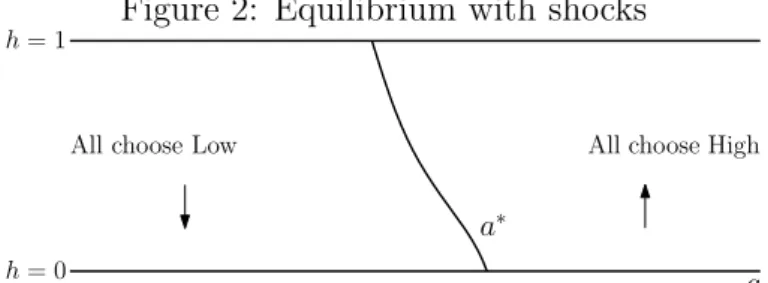
The equilibrium is characterized by a threshold. A largerhimplies that agents are willing to invest for lower values ofa, as in Figure2. Beliefs about others’ investment decisions are pinned down by fundamentals (a) and history (h). Shocks to atand movements in ht might
affect expectations about others’ actions.
Figure 2: Equilibrium with shocks
All choose Low
a h= 1
h= 0
All choose High
a∗
LetV(a, h,˜a) be the utility gain from choosingHigh obtained by an agent in state (a, h) that believes others will play according to threshold ˜a. Then
V(a, h,˜a) =
ˆ ∞
0
e−(ρ+α)tE[π(ht, at)|a, h,˜a]dt−ψ, (10)
whereE[π(ht, at)|a, h,a˜] denotes the expectation ofπ(ht, at) of an agent in state (a, h) that
believes others will play according to a threshold ˜a. An agent choosing whena=a∗(h) and
12We have shown instantaneous payoffs are increasing inaandhand an argument similar to the proof of
Proposition1 can be used to show that investing is a dominant action for high enoughaand a dominated action for low enougha. We will show the existence of dominance regions for a more general process forat
believing all others will play according to the cutoffa∗ is indifferent betweenHigh and Low,
which means that V(a∗(h), h, a∗) = 0, for every h.
4
The planner’s problem
Proposition 2 shows there is a unique rationalizable equilibrium in the model. Although agents face a dynamic coordination problem, a unique set of rationalizable beliefs emerges and, from the point of view of an individual firm, pins down the optimal decision. It is then natural to ask about the beliefs that arise in equilibrium and, in particular, about the inefficiencies that might exist in the model.
One particularly important question is about whether inefficiencies are more pronounced at times of low economic activity. For instance, suppose the current value of h is low and the economy is at the left but close to the equilibrium threshold. A firm chooses not to invest and the economy might be stuck in a regime with low economic activity for a while. Is that situation particularly inefficient? Would a social planner be particularly interested in stimulating investment whenh is low?
The planner maximizes expected welfare, given by:
Eτ(W) =Eτ ˆ ∞
τ
e−ρ(t−τ)(Y(ht, at)−αψI(t))dt (11)
whereY(h, a) is given by (7) andI(t)∈[0,1] is the decision of the planner about investing at timet.
The path ofa is exogenously given and the path ofh depends on future decisions of the planner, which is taken as given by the planner at a certain point in time. The planner chooses investmentI(τ) at every point in time, which affectshin the following way: investing
dI today raises h by αdI, but that increase depreciates at rate α. Hence
dht
dI(τ) =αe
−α(t−τ)
The first order condition ofEτ(W) with respect to investmentI(τ) at a given timeτ implies
that the planner is indifferent between any level of investment if:
ˆ ∞
τ
e−ρ(t−τ)Eτ
∂Y(ht, at)
∂h αe
−α(t−τ) !
dt−αψ = 0
Since
∂Y(ht, at)
∂h =e
at θ
θ−1
htx θ−1
θ
H + (1−ht)x θ−1
θ L
θ1 −1
x
θ−1 θ H −x
θ−1 θ L
we get that the planner chooses to invest at timeτ (I(τ) = 1) if:
ˆ ∞
τ
e−(ρ+α)(t−τ)E
τ "
θ
θ−1π(ht, at)
#
dt ≥ψ (12)
where π(ht, at) is given by (8). That is a necessary condition for optimality. In principle,
it is difficult to characterize the planner’s solution because expectations about the path of (a, h) have to be taken into account in the solution for the optimal decision but the path of
h will be optimally chosen by the planner.
However, mathematically, this problem is very similar to the agent’s problem in the decentralized equilibrium. At every point in time, there is investment if (12) holds, taking into account that the path of h in the future will be determined by a similar choice. The only difference is that the planner and agents follow different decision rules, but even that difference is small: the expression for the planner’s choice in (12) and the expression for a firm’s decision in (9) differ only by the termθ/(θ−1) multiplying the benefit from investing in (12). Hence we know the planner also chooses according to a thresholda∗
P such that (12)
holds with equality at a∗
P(h) forh∈[0,1].
The key implications for the optimal stimulus policies are in Proposition 3:
Proposition 3. Optimal policy:
1. [Optimality of a constant subsidy] The planner’s solution can be implemented by a constant subsidy of ψ/θ whenever an agent invests.
2. [Parallel shift of the threshold] The planner invests according to a threshold a∗ P such
that for any h∈[0,1],
a∗
P(h) = a∗(h)−log
θ θ−1
!
where a∗ is the threshold for the decentralized equilibrium.
Proof. First statement: The solution to the planner’s problem prescribes investment if (and only if) the condition in (12) is satisfied. Multiplying both sides of (12) by (θ−1)/θ yields the condition for an agent to invest in (10) in an economy where the cost for investing is
ψ−ψ/θ.
Second statement: Since π(ht, at) can be written as eatg(ht), for some function g(·), we
can rewrite condition 12as
ˆ ∞
τ
e−(ρ+α)(t−τ)E
τ
e(at+log(θθ
−1))g(ht)
dt≥ψ (13)
Define bt = at + log
θ θ−1
decisions in the decentralized equilibrium (in the (a, h)-space). Moreover, the law of motion forbtis exactly the same as the law of motion forat. Therefore, the solution for the problem
must be the same as well.
We know there is a unique decentralized equilibrium given by a threshold a∗, hence
a∗ =b∗, which implies a∗(h) = a∗
P(h) + log
θ θ−1
and yields the claim.
Figure 3: Planner’s problem
a h= 1
h= 0
a∗
a∗
p
The solution to the planner’s problem in (12) considers the benefits from investing by an individual producer multiplied by a constant larger than 1. Hence the only problem with the individual decision is that it requires a benefit from investing that is too high. A constant subsidy takes care of this problem.
As shown in (13), the expressions for the planner’s problem in (12) is the same as the solution for the decentralized problem in (10) when a constant is added to the log of productivity. That implies the planner’s threshold is a translation of the equilibrium threshold, where that constant is subtracted from the productivity threshold, as in Figure
3.13
The slope of the threshold affects the likelihood of a recession and its expected duration. If the threshold is close to a vertical line, h will start to fall when productivity is below some a† but firms will resume investing whenever a
t> a†. A rotation of the threshold that
reduces a∗(1) but raises a∗(0) implies there will be less ocasions where productivity will
cross the threshold to the left of a∗ when h is large, but when that happens, h is likely to
go further down and it will take longer for h to increase again.
An implication of Proposition 3 is that a constant subsidy implements the planner’s solution if and only if the planner is not willing to affect the slope of the equilibrium threshold. The proposition shows the planner is not concerned with the timing of stimulus
13This analysis ignores the costs of subsidizing investment but the result is robust to the inclusion of
policies: there is no special reason for subsidies at times of low (or high) economic activity (h); and there is no reason to affect the expected duration of recessions.
The planner’s solution prescribes no extra stimulus for investment whenhis low because equilibrium beliefs solve the dynamic coordination problem. The next section provides economic intuition for this result.
5
Understanding the result
Suppose the economy is ath= 0 and at the left but very close to the equilibrium threshold. Agents are stuck in a regime with low economic activity but would choose to invest if the economy switched to a high-h state. The planner could drive the economy to higher values of h but, as we’ve shown, this dynamic coordination problem does not provide a reason for stimulus at low h. Why?
The explanation can be divided in two parts: (i) the externality from investing is always a constant proportion of the individual return; and (ii) equilibrium beliefs compensate for the dynamic coordination problem. For the first part, note that welfare in this economy at time t can be written as W(h, a) = hwH(h, a) + (1−h)wL(h, a). That yields:
∂W
∂h = (wH(h, a)−wL(h, a)) + h
∂wH(h, a)
∂h + (1−h)
∂wL(h, a)
∂h
!
An agent takes into account the effect of investment on her income but not the positive effect on others from selling at a lower price. However, owing to the constant demand elasticity,
h∂wH(h, a)
∂h + (1−h)
∂wL(h, a)
∂h
!
= 1
θ−1(wH(h, a)−wL(h, a))
The externality is a constant proportion of the agent’s payoff from investing and, conse-quently, independent of h or a for a given return to investment. Non-proportional exter-nalities in payoffs may generate non-constant optimal subsidies but for reasons unrelated to the dynamic coordination problem. Sections 5.4 and 5.5 discuss how the model is affected when the externality depends onh.
5.1
Solutions for
σ
= 0
and
σ
→
0
+The uniqueness result and the expressions for the equilibrium and planner’s thresholds hold for any σ >0. In case σ →0+, the expression for the threshold can be simplified. For any
h0 ∈ [0,1], suppose the economy is at the threshold, i.e., at (a∗(h0), h0). The economy will
soon move either up or down, but how exactly does it work and what are the probabilities the economy will go in each direction? This mathematical problem is studied by Burdzy et al. (1998) and their main result is that the economy will instantaneously move up in the direction of (a∗(h
0),1) with probability 1−h0 and will move down in the direction of
(a∗(h
0),0) with probability h0. Using (10), a∗0 ≡a∗(h0) thus solves:
(1−h0) ˆ ∞
0
e−(ρ+α)t[π(h↑t, a∗0)]dt+h0 ˆ ∞
0
e−(ρ+α)t[π(h↓t, a∗0)]dt =ψ (14)
where h↑t = 1−(1−h0)e−αt, and h↓t = h0e−αt. The solution to the planner’s problem is
similar. Using (12), we get that for any h0 ∈ [0,1], the planner’s threshold a∗P0 ≡ a∗P(h0)
solves:
(1−h0) ˆ ∞
0
e−(ρ+α)t[π(h↑
t, a∗P0)]dt+h0 ˆ ∞
0
e−(ρ+α)t[π(h↓
t, a∗P0)]dt =ψ−
ψ
θ (15)
For the planner, there is no difference between no shocks (σ = 0) or vanishing shocks (σ → 0+). Beliefs about the future are basically the same and the planner can effectively
choose the path of h.14
However, the decentralized equilibrium in case σ= 0 can be very different from (14). In case of optimistic beliefs, the agent’s thresholda∗
opt solves: ˆ ∞
0
e−(ρ+α)t[π(h↑t, a∗opt(h0))]dt=ψ (16)
for every h0, while in case of pessimistic beliefs, the agent’s threshold a∗pes is given by: ˆ ∞
0
e−(ρ+α)t[π(h↓t, a∗pes(h0))]dt=ψ (17)
The irrelevance of vanishing shocks for the planner’s solution highlights the point that
14The planner’s problem with σ = 0 can be written in a different way: the planner chooses between
always investing and never investing in the foreseeable future (any other option is dominated by one of these alternatives). Thusa∗
P0 solves:
ˆ ∞
0
e−ρthh↑
twH(a∗P0, h↑t) + (1−h
↑
t)wL(a∗P0, h↑t)−h
↑
tψ˜
i
−hh↓twH(a∗P0, h↓t) + (1−h
↓
t)wL(a∗P0, h↓t)−h
↓
tψ˜
i dt= 0
very small fluctuations inaare not intrinsically important. Their effects on the decentralized equilibrium stem from the determination of beliefs in caseσ →0+.
5.2
The case with no shocks
Consider the case σ = 0. The equilibria of the model are depicted in Figure 4. The left threshold (good equilibrium) is the set of (a, h) where an agent is indifferent between investing or not assuming all others will invest given by (16). For the right threshold (bad equilibrium), the assumption is that no other agent will ever choose to invest, as in (17).
Figure 4: The case with no shocks
a
h= 1
h= 0
Planner Good equilibrium Bad equilibrium Beliefs Problem
Dynamic Problem
There are three differences between the planner’s solution and the decentralized equilib-rium: (i) the solution for the planner’s problem is unique but there are multiple self-fulfilling equilibria; (ii) the planner takes into account the price externality from market power; and (iii) in the decentralized equilibrium, agents face a dynamic coordination problem: in a re-gion of parameters, nobody wants to be the first to invest although investing is the socially optimal choice.
There are multiple equilibria in a region of parameters (the first difference between the planner’s solution and the decentralized economy). However, regardless of whether we assume optimistic or pessimistic beliefs, the equilibrium threshold is further away from the planner’s threshold for low values of h. The difference in slopes shows the planner would be willing to pay higher subsidies when h is low – as shown in Proposition 3, a constant subsidy would shift the threshold to the left without rotating it. That is the third difference between the planner’s solution and the decentralized economy.
happy to sign a contract forcing everyone to take investment opportunities in the short run, as these losses for some would imply gains for all in the future.
While the planner effectively decides where the economy goes, agents take beliefs as given. In consequence, the economy might be stuck in a recession trap (low h, not so low
a). However, beliefs are exogenous in this reasoning. We now consider the case of a positive but very smallσ to understand which beliefs arise in equilibrium.
5.3
The case with very small shocks
We now consider the case withσ →0+. Differently from the previous case, beliefs now are
uniquely determined by the model. The equilibrium is depicted in Figure5.
Figure 5: The case with very small shocks
a
h= 1
h= 0
Planner
Good equilibrium
Bad equilibrium Unique equilibrium
with shocks Externality problem
The result is completely different from the case with σ= 0. As in Frankel and Pauzner
(2000), with very small but positive shocks, there is no role for arbitrary beliefs and no multiplicity of equilibria, so the first difference between the planner’s problem and the decentralized equilibrium disappears. The surprising result from this paper is that the difference in slopes between the planner’s and the agents’ thresholds vanishes as well.
Since the productivity parameter moves very slowly, this change in the behavior of the economy must stem from the endogeneity of beliefs. As shown in Figure5, the equilibrium threshold ath= 0 coincides with the ‘good’ equilibrium of the model with no shocks, hence agents are very optimistic at h = 0. The same reasoning also implies that agents are very pessimistic at h= 1.15
Intuitively, in a neighborhood of the equilibrium threshold, optimistic beliefs make per-fect sense at h = 0, but no sense whatsoever at h = 1. Suppose the economy is exactly at the equilibrium threshold at h = 0. The economy would stay around there as long as
a < a∗(0), but any shock that moves a above a∗(0) leads agents to invest and drives the
15An implication ofBurdzy et al. (1998) is that in caseσ→0
economy up in the picture. Since the slope of the threshold is negative, as soon as the economy is at h >0, it is at the right of the threshold and hence moves up in the direction of h = 1. The fundamental asymmetry here is that a tiny negative shock basically leaves the economy where it is, while a tiny positive shock drives the economy up in the direction of h = 1. The same reasoning implies that in a neighborhood of the equilibrium threshold ath= 1, a regime switch is also expected and beliefs are pessimistic.
The intuition for equilibrium beliefs was explained for the case with σ→0+ but
Propo-sition 3shows the result holds for any σ >0. Graphically, for σ bounded away from 0, the planner’s and agents’ equilibrium thresholds would be parallel to each other as in Figure5, but the agents’ threshold would not touch the boundaries of the dominance regions.
The intuition for the case with σ bounded away from zero is very similar. When eco-nomic activity is low and agents are around the equilibrium threshold, they are optimistic: productivity is relatively good, the economy is parked in a region of inaction but is likely to leave that state soon. Again, the key asymmetry here is that a movement of a to the left does not significantly affect the state of the economy, but a movement ofa to the right affects the mass of agents investing, raising demand in the economy and incentives for the following agents with investment opportunities to take them. The recovery is just waiting for a small piece of good news.
The only difference between the planner’s solution and the decentralized equilibrium is the monopoly distortion in the investment decision, the externality shown in Figure 5. When beliefs are determined by the model, planner and agents solve a very similar problem. At every (a, h), investment is undertaken if its expected return pays off and the equilibrium (or planner’s) threshold is a fixed point. “Pays off” means different things for agents and planner but the ratio is constant since the only difference is the externality from market power.
5.4
What if the externality is not a constant fraction of payoffs?
Different functional forms for preferences and technology could in principle lead to exter-nalities varying withh. We now argue that for reasonable parameters (namely forρ << α), the effect of, say, larger externalities for low values ofh would be mitigated in equilibrium. Consider the caseσ →0+, assume the private gain from investing is π =eag(h) and the
planner’s instantaneous gain is:
Λ(h, a)≡[1 +κ]eag(h) +β(h) with
ˆ 1
0
β(h)dh= 0
the planner’s threshold in (15) yields:
aP(0) = log
αψ
´1
0(1−h)ρ/αea(1 +κ)g(h)dh+ ´1
0(1−h)ρ/αβ(h)dh
(18)
and
aP(1) = log
αψ
´1
0 hρ/αea(1 +κ)g(h)dh+ ´1
0 hρ/αβ(h)dh
(19)
The second integral term in the denominator of both (18) and (19) corresponds to devia-tions from a parallel shift of the threshold – if that term is 0, deviadevia-tions from the average externality do not show up in the equations. In general, the second integral terms in (18) and (19) will be small for two reasons: (i) β(h) is the difference between the externality at a particular value of h and the mean externality (across h), while ea(1 +κ)g(h) is the
private gain plus the average externality, which would in general be much larger; and (ii)
ρ/αtends to be small sinceρis the time discount rate (say 2% a year) andαis the frequency agents choose investment (say twice a year). Hence there will be little dispersion on weights attached to eachβ(h) and the second integral will therefore be close to 0.
The second point is particularly related to our main contribution, so it is worth exploring it with an illustration. We now consider a linear example so thatβ(h) = ζ−2ζh, hence the externality is larger at h= 0 by ζ. In this case
ˆ 1
0
(1−h)ρ/αβ(h)dh= ζρ/α
(1 +ρ/α) (2 +ρ/α) <
ζ
2
ρ α
In words, the “extra” externality ath= 0 has to be divided by two and multiplied by ρ/α. This term is then added to the denominator of the expression for aSP(0) in (18) (and a
similar term is subtracted from the expression for aSP(1)). Since the time discount rate ρ
is in general much smaller than the frequency of decisions α, only a small fraction of the “extra” externality at h = 0 is considered in the expression for aSP(0). Intuitively, when
deciding on investment at the equilibrium threshold ath= 0, the planner takes into account that the economy will soon be moving up, so the “local” externality is not that important.
5.5
The case with vanishing frictions
In case of vanishing frictions (α → ∞), the economy moves very fast from h = 0 to h = 1 but agents’ horizons become very short.16 In the model with no shocks, agents take h
into account in their decisions, regardless of whether we assume fully optimistic or fully pessimistic beliefs. In contrast, the planner does not take hinto consideration. Moving the
economy to a different regime takes very little time and hence the transition is unimportant. The threshold from the planner’s problem converges to a vertical line, as in Figure6. This result holds for any σ >0.
Figure 6: The case with vanishing frictions
a
h= 1
h= 0
Planner
Good equilibrium
Bad equilibrium Unique eq.
with shocks Externality Problem
An implication of Proposition 3 is that in equilibrium agents also play according to a vertical threshold. History thus becomes irrelevant.17 Interestingly, this result holds even in
case of non-proportional externalities as discussed in Section5.4. Whenα→ ∞, the second integral in the denominators of (18) and (19) converge to zero, hence the differences in the externality from the High regime across h do not affect the planner’s or agents’ decisions. Hence for large α/ρ, the optimal policy prescribes an approximately constant subsidy even if externalities are larger when h is low.
6
Extensions
6.1
A macroeconomic model with labor
The underlying macroeconomic model presented in Section2is quite stylized. Firms cannot adjust their production in the intensive margin when economic conditions change. In this section we develop a standard macroeconomic model where firms still receive opportunities to increase their productivity according to a Poisson process, but can adjust the amount of labor used in production at each point in time. The qualitative results in Proposition3 are
17Intuitively, for a largeα, an agent at the equilibrium threshold andh= 0 knows the economy will move
up with probability 1, while an agent at the equilibrium threshold andh= 1 is sure the economy will move down. They don’t know their ‘position in the queue’, i.e., when they will have the next opportunity for revising their behavior: how much time will have elapsed and the value ofhwhen they can choose again. On the one hand, the agent ath= 0 will experience lower values of hthan the agent ath= 1 – the agent starting ath= 0 is likely to get an opportunity to revise behavior beforehgets close to 1. On the other hand, for the agent at h = 0, the economy moves up very quickly at lower values of h, but slowly as h
approaches 1, so the last firms to change their decision will spend relatively more time at high values of
unchanged, i.e., the constant subsidy is still optimal and the planner chooses a threshold that is parallel to the agent’s threshold.
There is a continuum of intermediate good firms indexed byi∈[0,1] and a representative household who supplies labor and consume a final good. The final good is produced by a competitive firm whose production function is the Dixit-Stiglitz aggregator of intermediate goodsyit, given by equation (1) as before. The price of the final good is Pt. The household
utility function is given by
U(Ct, Lt) = Ct−
1
γ+ 1L
γ+1
t ,
whereCt is the amount consumed of the final good,Ltis the total amount of labor supplied
and γ ≥ 0 parameterizes the Frisch elasticity of the labor supply. The household budget constraint is
PtCt≤wtLt+ ˆ 1
0
Πitdi,
where wt is the wage and Πit is the profit of firm i (the household owns all the firms).
As before, at a given point in time, intermediate good firms can be in either theHigh (H) or the Low (L) regime and opportunities to switch across regimes follow the same Poisson technology as in Section 2. Firms use labor to produce their differentiated goods. A firm i
in regime r∈ {L, H} has production function
yit =AtXrlλit,
where lit denotes the amount of labor used in production, λ ∈ (0,1) and XH > XL.
In-termediate good firms maximize profit taking the demand schedule imposed by final goods firms as given. The stochastic process ofat= log(At) is the same as in Section 2.
6.1.1 The agent’s problem
We will start solving for the equilibrium in a given period t taking the proportion of firms in each regime as given. Since firms in a given regime and at a point in time make the same choices in equilibrium, we will abuse notation and index firms by the regime r ∈ {L, H}. We will also omit time subscripts in this subsection.
The demand schedule of the final good firm is the same as before and is given by (4). Therefore, we can write the profits of a firm in regime r as
Πr =y θ−1
θ r Y
1
θ −w
y
r
AXr λ1
For a given wagew and final good output Y, the optimal choice of a firm in regime r is:
yr = "
θ θ−1
!
1
λ
#−θλζ
(AXr)θζYλζw−θλζ, (21)
where ζ ≡ 1
λ+θ(1−λ). A firm producing yr will demand lr = [yr/(AXr)] 1/λ
units of labor. For a given wagew, the household will supply w1/γ units of labor. Thus, equilibrium in the
labor market implies:
w= " h y H AXH λ1
+ (1−h)
y
L
AXL 1λ#γ
. (22)
Finally, goods markets must clear:
Y =
hy
θ−1 θ
H + (1−h)y θ−1
θ L
θθ −1
. (23)
Equations (21), (22) and (23) pin down the equilibrium of this economy for a given state (a, h). From these equations, we find equilibrium expressions for the final good production
Y(h, a), the production for firms in each regimeyH(h, a) andyL(h, a), and the wagew(h, a).
These lead to expressions for hours workedL(h, a) and profits ΠH(h, a) and ΠL(h, a).
The final good production in equilibrium is given by:
Y(h, a) =
"
θ θ−1
!
1
λ
#λ λ −γ−1
exp
(
γ+ 1
γ+ 1−λ
!
a
)
q(h)λγδ(γ+1)(θ−δ1)−−11, (24)
where q(h) ≡ hh(XH)(θ−1)ζ + (1−h) (XL)(θ−1)ζ i
and δ ≡ 1
(1+γ)θ−(θ−1)λ. The difference in
profits between firms in regimeHigh and Low:
˜
π(h, a) = exp
(
γ+ 1
γ+ 1−λ
!
a
)
q(h)λγ(θ(−θ1)(−1)λ−−(γγ−+1)1)
XH(θ−1)ζ−X
(θ−1)ζ L
Φ, (25)
where Φ≡hθ−θ11λi
λ λ−γ−1
−hθ−θ1
1
λ iλγ+1
−γ−1
.
It is no longer true that the gain of being in regime High above is always increasing in
h. We need to impose the following restrictions on parameters:18
λ(θ−1)−1<1/γ (26)
This restriction is satisfied for standard parameters in the literature.19 Notice that the Frisch 18Ifγ= 0 we cannot write this assumption this way, but the condition is always satisfied.
19For example, the restriction is satisfied withθ= 5,λ= 2/3 andγ= 1/3. For a recent discussion about
elasticity 1/γ cannot be too low relative to θ, which determines the intensity of demand externalities in the economy. As in the model of Section 2, when others produce more, an agent is more inclined to incur the fixed cost for the High regime, owing to the increase in price of his variety. However, in the model with labor, there is also an effect in the opposite direction: when others are in regime High and producing more, wages increase as well. If the Frisch elasticity is high, then the effect on wages is small and the overall incentives to be in regime High increase in h. Finally, λ also enters the expression since it affects the difference in labor used by firms in each regime.
Given that the assumption in (26) is satisfied, the equilibrium of the dynamic game is given as in Section3, with π(h, a) replaced by ˜π(h, a) from (25).
6.1.2 The planner’s problem
The planner seeks to maximize the discounted sum of flow payoffs of the representative household, which is given by USP =Y − 1
γ+1L
γ+1. There are two different ways to consider
the planner’s problem: (i) the planner chooses whether firms invest and how much labor they hire (and hence how much they produce); or (ii) the planner will not interfere in firms’ pricing decisions and in workers’ labor supply, will only choose investment. Since we are concerned with policies to stimulate investment, we now focus on the second alternative, but the first one is presented in the appendix and the results are essentially the same as in Proposition3.
The planner thus determines the choices of firms between the High and Low regimes, taking as given what firms and workers will choose at every point in time. The flow utility of the representative household can thus be rewritten as
USP(h, a) =hΠH(h, a) + (1−h)ΠL(h, a) +
γ
γ+ 1w(h, a)
γ+1
γ . (27)
where functions Y(h, a), L(h, a), ΠH(h, a), ΠL(h, a) and w(h, a) refer to the decentralized
equilibrium of this economy for a given h and a, as defined in the last subsection.
Repeating the steps leading to (12), we get that the solution to the planner’s problem can be written as the solution to the decentralized equilibrium replacing the private gain from being in the High regime ˜π(h, a) by ∂USP
∂h . Taking partial derivatives of (27) with
respect toh, using (22) and the equality between marginal revenue and marginal cost, and rearranging, we get:
∂USP(h, a)
∂h = ˜π(h, a) +
1
θ
∂Y(h, a)
Taking derivatives of (24) and rearranging leads to:
∂USP
∂h =
1 1−χ
!
˜
π(h, a),
where χ= θ− λ1 γ+1(θ−1)
.
Following the steps in Section4, we can show that a constant subsidyχψ implements the planner’s first best.20 Moreover, the planner’s threshold is parallel to the agent’s threshold
and given by
˜
a∗
P(h) = ˜a∗(h)−
γ+ 1−λ γ+ 1
!
log 1 1−χ
!
, (28)
where ˜a∗(h) denotes the agent’s threshold in the model of this section.
6.2
Implementation
Proposition3 shows that a constant subsidy implements the first best. However, in a large set of states, much less generous subsidies would be enough to coax agents to invest. This leads to the following question: what if every unit of subsidy has a small welfare costε≈0? It is not difficult to show that the government will use minimal spending policies, as in Definition1.
Definition 1. Leta∗ be an equilibrium of the game anda∗
p a continuous function such that
a∗
p(h) < a∗(h), for every h. Let ˆa be the boundary where an agent is indifferent between
High and Low when others are playing according toa∗
p. The functionϕ(h, a) is theminimal
spending policy that implements a∗ p if
ϕ(h, a) =
ψ−´∞
0 e
−(ρ+α)tE[π(h
t, at)|a, h, a∗p]dt if a∗p(h)≤a≤ˆa(h)
0 otherwise . (29) Figure7shows 3 thresholds: a∗
p is the threshold implemented by the policy, ˆa is the best
response of a player that believes others will play according to a∗
p and a∗ is the equilibrium
threshold without intervention. By definition, a∗ is the best response to others playing
according to a∗. Now, the sheer change in beliefs affects agents’ strategies: once they
believe others will play according toa∗
p, they will be indifferent betweenHigh and Low at a
threshold ˆa such that ˆa(h)< a∗(h) for allh
∈[0,1].
A government following a minimal spending policy is committed to give an investment subsidy to each agent in the region between a∗
p and ˆa (the gray area in figure 7). The
20When the planner can affect not only investment but also labor and production at eacht, the optimal
Figure 7: Example of minimal spending policy
a h= 1
h= 0
a∗
a∗
p aˆ
subsidyϕ(h, a) makes her indifferent between choosingHigh and Low given others will play according to a∗
p. Under those beliefs, playing according to a∗p is a best response under this
policy, soa∗
p is an equilibrium. Interestingly, no subsidies are needed in the area between ˆa
and a∗.21
Proposition4shows that minimum spending policies do not affect the main result of the paper.
Proposition 4. In the model of Section 2 with minimal spending policies, the maximum optimal subsidy is ψ/θ for all h∈[0,1].
Proof. See AppendixB.
The result is intuitive. Under minimal spending policies, investment subsidies are equal to the minimum between how much the planner is willing to pay and how much is required to coax agents to invest. The result from Proposition 4 thus follows from the planner’s willingness to subsidize being independent ofh (Proposition 3).
6.3
Mean reversion
We now consider at follows a process with mean reversion. Let at = log(At) vary in time
according to
dat=η(µ−at)dt+σdZt (30)
The parameter η determines how fast at returns to its mean, given by µ. Proposition 5
builds on Frankel and Pauzner (2000) to show that a threshold equilibrium always exists.
Proposition 5 (Existence). Suppose σ > 0. There exists a strictly decreasing function a∗
such that a∗ is an equilibrium.
21The equilibrium under the minimal spending policy is no longer unique. If agents believe others will play
Proof. See AppendixB.
The first statement of Proposition 3 still holds when the process for at exhibits mean
reversion, thus the planner’s solution can be implemented by a constant subsidy. However, the second statement does not hold in this case because with mean reversion, translating the threshold is not isomorphic to re-labeling the a-axis. A translation of a∗ also implies
a different path ofat and, consequently, a different balance between expected demand and
productivity around that threshold. However, numerical results show that for a reasonable amount of mean reversion, the results are essentially unchanged.22
We do not have a strong uniqueness result in this case. However, the model can be seen as a limiting case of a sequence of models that have a unique rationalizable equilibrium. The following section discusses this point.
6.3.1 On equilibrium uniqueness
In order to apply the results of Frankel and Burdzy (2005), we need to make two changes in the model. First, the diffusion process for at is given by (30), but the mean-reversion
parameter ηt varies over time so that
ηt =
η if t < T
0 otherwise, (31) where T is a large number. Second, the difference between the instantaneous utility of agents locked in each regime is given by ˆπ instead ofπ, where
ˆ
π(h, a) =
π(h, a) if a < M
π(h, M) otherwise , (32) where M is a large number. One can verify that ˆπ(h, a) is Lipschitz in both a and h, and continuous. Using the results inFrankel and Burdzy(2005), we can prove there is a unique equilibrium in this model.
Proposition 6 (Uniqueness, Frankel and Burdzy(2005)). Suppose σ >0, the mean rever-sion parameterηt is given by (31) and the relative payoff of investing is given by (32). Then
there is a unique rationalizable equilibrium in the model. Agents follow cut-off strategies, and the cut-off can vary over time.
Proof. See AppendixB.