Selection of productivity improvement techniques via mathematical modeling

(1)

Management Science Letters 1 (2011) 379–388

Contents lists available atGrowingScience

Management Science Letters

homepage: www.GrowingScience.com/msl

Selection of productivity improvement techniques via mathematical modeling

Mahassan M. Khatera and Noha A. Mostafaa*

a

Department of Industrial Engineering, Zagazig University, Zagazig, Sharkeya, Egypt

A R T I C L E I N F O A B S T R A C T

Article history:

Received December 20 2010 Received in revised form 23 January 2011

Accepted 23 January 2011 Available online 25 January 2011

This paper presents a new mathematical model to select an optimal combination of productivity improvement techniques. The proposed model of this paper considers four-stage cycle productivity and the productivity is assumed to be a linear function of fifty four improvement techniques. The proposed model of this paper is implemented for a real-world case study of manufacturing plant. The resulted problem is formulated as a mixed integer programming which can be solved for optimality using traditional methods. The preliminary results of the implementation of the proposed model of this paper indicate that the productivity can be improved through a change on equipments and it can be easily applied for both manufacturing and service industries.

Keywords: Productivity

Productivity improvement Optimization

Integer programming (IP) and Multiple regression

1. Introduction

Productivity is a ratio measuring how well input resources are converted into outputs. Productivity management aims at developing plans for productivity programs, which are based on productivity cycle of four stages: measurement, evaluation, planning and improvement (MEPI) as shown in Fig.1. Productivity program is a continuous process. Therefore, productivity improvement must be preceded by measurement, evaluation and planning.

(2)

measures. Partial productivity is a ratio of output to one class of inputs. Total-factor productivity is the ratio of net output to sum of associated labor and capital inputs. Net output is total output minus intermediate goods and services purchased. Total productivity is the ratio of total output to sum of all input factors. Total productivity model (TPM) is based on a total productivity measure and a set of five partial productivity measures and it is a good diagnostic tool for productivity improvement. Productivity evaluation is normally treated as a complementary part of productivity measurement and it is evaluated by means of productivity indices calculated in productivity measurement stage.

Productivity planning requires forecasting the level of total productivity in future time based on the past performance. Forecasting can be performed based on a simple linear trend model and it has the advantage of forecasting for productivity increase. Goodwin (1968), emphasized that improvement must be managed in deliberate manner. He attempted to answer a question on how we can improve the way improve. Sutermeister (1976) provided a descriptive model to view the interaction of several factors in affecting employee productivity. He identified two major categories: technological development and employee motivation. Hershauer and Ruch (1978) presented a servo system model of employee productivity considering the individual worker performance as the focal point of the model. Their model's difficulty in practical usage is the inability to quantify the behavioral and marginal factors, which leads to sub-optimization in total productivity improvement. Crandall and Wooton (1978) presented a model that integrates the role of productivity improvement with the growth of the organization. They identified four possible sequential stages of organizational growth and specified three basic types of productivity strategies for each of the four growth phases of an organization. This specification seems logical, though not empirically tested.

Stewart (1978) proposed a productivity improvement strategy for organizations based on system perspective described in twelve steps. Based on the analysis of twenty-seven published case studies, Aggarwal (1979) proposed a step-by-step procedure to productivity improvement in companies composed of nine steps. Sink (1982) proposed a motivation-oriented productivity improvement model, which is worth pursuing in empirical testing. Sumanth and Yavauz (1983) proposed an analytical model, which was later adapted by Sumanth (1984). The model is based on a scientific selection of a set of improvement techniques for a given time period to achieve the best level of total productivity. In addition, the selection techniques vary according to availability of funds to install the techniques and the payback associated with such selection. Sumanth (1984) classified fifty-four improvement techniques into five basic categories. These categories are: Technology-based techniques, Employee-based techniques, Product-based techniques, Task-based techniques and Material-based techniques.

(3)

M. M. Khater and N. A. Mostafa / Management Science Letters 1 (2011)

381

2. Productivity cycle

Productivity cycle is the base of productivity programs. This cycle is composed of four continuously cycling stages (MEPI).

2.1Productivity measurement

Measurement part is an essential stage as it has several benefits. Basic productivity types are partial productivity, total-factor productivity and total productivity. Although data gathering for total productivity computations is a relatively difficult task, it is more accurate and representative since it considers all quantifiable output and input factors. There are different models for productivity measurement, but most of them have limitations (Sumanth, 1984). Total productivity model (TPM) has many advantages both diagnostic and prescriptive. This model lends itself to productivity evaluation, planning and improvement in a scientific manner and it has many applications for manufacturing or service organizations. Total productivity model is a basic model based on a total productivity measure and a set of five partial productivity measures: labor, material, energy, capital and other expenses (L, M, E, C, X) measures. As TPM mix total and partial productivity measures, it can be a good diagnostic tool for productivity improvement. (Nawara & Mostafa, 1991). Productivity measures can be computed using the following relationship. Total productivity (TP) defined in TPM is given by

TP = Total tangible output / Total tangible input. (1)

Let O be total tangible output as follows,

O = value of finished units produced + value of partial units produced + dividends from … securities + interest from bonds + other income,

(2)

and let I be total tangible input as follows,

I = value of [L + M + E + C + X] inputs used. (3)

All outputs and inputs are expressed in the same monetary terms of a base period (0). Therefore, for a current period (t),

TPFt = OFt / IFt =

∑

= N

i1

Oit /

∑

= N

i1

Iit ,

(4)

TPF0 = OF0 / IF0 =

∑

= N

i1

Oi0 / Ii0 ,

(5)

where,

TPF = total productivity of a firm;

TPi = total productivity of product i in the firm, i = 1,2…N;

N = total number of products manufactured in the firm during a considered period;

OF = total output of a firm; and

IF = total input of a firm.

Ii =

∑

j

Iij = IiL + IiM + IiE + IiC + IiX,

(6)

Iij = input of type j for product i

(TPIF)t = total productivity index for the firm in period t = TPFt / TPF0. (7)

(TPI)i = total productivity index for product i in period t = TPit / TPio .

…

(8)

∑

= N

(4)

Sumanth (1984) introduced the following mathematical model for evaluating productivity between two periods t-1 and t.

ΔTPit = change in total productivity of product i in period t with respect to period t-1

ΔTPit = (ΔOit – ΔIit . TPit-1)/ (Iit-1 + ΔIit) . (9)

ΔTPit < 0, means that total productivity has decreased in period t as compared to period t-1.

ΔTPit = 0, means that total productivity remained constant between periods t-1 and t.

ΔTPit > 0, means that total productivity has increased in period t as compared to period t-1.

2.3Productivity planning

In this part, short-term productivity planning (SPP) will be used for monitoring productivity changes and controlling productivity levels. To forecast the level of total productivity in future times based on the past performance, the linear trend model will be used as its theory is well established. This model can forecast for an increase in productivity at a certain rate by assuming linear trend. Therefore, double exponential smoothing (DES) is an adequate method to forecast total productivity in the coming period. Besides, there are many available tools to perform any computations needed.

2.4Productivity improvement

The productivity improvement approaches mentioned in section 1 are limited in their abilities to provide a pragmatic tool to monitor productivity changes. In addition, most of these approaches do not emphasize the need of improving total productivity and they cannot provide a mathematical model associated with productivity improvement level to productivity improvement techniques.

The improvement techniques are various and can be classified into five basic categories (Sumanth, 1984):

I. Technology-based techniques, such as Computer integrated manufacturing (CIM),

II.Employee-based techniques, such as Management by objectives (MBO),

III. Product-based techniques, such as Advertising and promotion,

IV. Task-based techniques, such as Job safety design,

V. Material-based techniques, such as Inventory control.

It is desirable to determine which of the improvement techniques should be used, so that the total productivity of an organization is optimally improved. The model must be based on scientific selection of a set of techniques such that an analysis can be performed to determine the changes on the selection based on the target level of total productivity, the availability of funds to install the techniques and the payback associated with such selection. The analytical productivity improvement model (APIM) adopted by Sumanth (1984) is recommended in this paper.

3. Analytical productivity improvement model (APIM)

The proposed model of this paper first collects the necessary data and structure for the purpose of multiple regression models. Next, the model investigates the coefficients obtained from the multiple regression models. The positive coefficients are then used as part of mixed integer programming model and the negative coefficient are investigated for possible reasons.

3.1Step 1: Data collection

Two types of information can be obtained from the organization:

1. Total ales and total expenses for the previous periods to estimate the total output and total input, respectively.

(5)

383

3.2Step 2: Preparing data file structure

The percentage change in total productivity between time periods t and t-1 (PCt) can be computed as,

PCt = [(TPt – TPt-1) / TPt-1] × 100. (9)

Then, a data file structure ,as shown in Table 1, can be prepared to record, at each time period t, (t = 1,2…n), the computed percentage change in total productivity (PCt) and the corresponding values of

the kth technique usage binary variable, Tk (k = 1,2…K, K = 54).

3.3Step 3: Multiple regression analysis

Assuming a linear relationship between the changes in total productivity and the usage of productivity improvement techniques in a given period t, PCt can be expressed as follows,

PCt = A0 +

∑

=

54

1 k

Ak Tkt ,

(10)

⎩ ⎨ ⎧ =

otherwise 0

period in used is technique if

1 k t

T_kt (11)

Ak = productivity improvement coefficient for technique k, k = 1, 2…54.

Coefficient Ak can be determined via multiple regression (Lapin, 1983). In this work, results are

computed with aid of CROSSTABS subroutine of statistical package SPSS using input data from data file obtained in step2.

3.4Step 4: Evaluation of productivity improvement coefficients and selecting candidate techniques

The techniques associated with positive coefficients are kept as candidate techniques and those associated with non positive coefficients are investigated to determine the reasons of their not contributing to organization total productivity improvement.

3.5Step 5: Selection of optimal candidate improvement techniques and sensitivity analysis

To determine the optimal improvement techniques for a given period, an integer programming (IP) model is proposed where the objective function is a linear function in candidate techniques usage variables with their positive predetermined coefficients. There are also some constraints associated with the model as follows,

Integer Programming model

∑

= r

k k kT

A

1

max (12)

subject to

Table 1

Data file structure

Time period t PCt T1 T2 … Tk … TK

1 PC1 0 or 1 0 or 1 … 0 or 1 … 0 or 1

2 PC2 0 or 1 0 or 1 … 0 or 1 … 0 or 1

… … … …

t PCt 0 or 1 0 or 1 … 0 or 1 … 0 or 1

… … … …

(6)

∑

=

≤

k k

kT F

f

1

,

∑

=

≥

r

k k

kT S

s

1

,

(14)

, ,..., 2 , 1 for

, k r

B T

b_k _k ≤ = (15)

, ,..., 2 , 1 for

, k r

M T

m_k _k ≤ =

{ }

0,1,

=

k

T (17)

where

Ak is the productivity improvement coefficients for technique k,

r is the number of candidate techniques, fk is the funds required for technique k,

F is the maximum available total funds, sk is the saving achieved using technique k,

S is the minimum acceptable total savings, bk is the payback period for technique k,

B is the maximum allowable payback period mk is the time required to install technique k,

M is the maximum allowable installation time.

3.6Step 6: Implementation of selected techniques

The techniques selected in step 5 will be implemented for the sake of the maximum possible improvement in total productivity level of the organization. An action plan must be drawn up for the proposed implementation. This action plan consists of three parts: logical framework (LF), project planning matrix (PPM) and objectives matrix. LF is a management tool that aims to state clearly the productivity improvement and components. PPM provides a simple and clear strategic plan to select appropriate techniques. For each technique, the following elements are defined.

Implementation elements:

Activities needed to implement the technique,

Expected completion time,

Resources needed,

Responsibility,

Concerned external organizations,

Implementations assumptions for external factors

Evaluation elements:

Verifiable indicators (Targets)

Means of verification

Objective matrix is a simple and effective way for performance measurement during different time horizon. It demonstrates the current state of the organization compared with the target level, and provides good criteria for evaluating the performance of the organization corresponding to the required techniques (Nawara, & Mostafa, 1991). Logically, after the implementation, total productivity level will be measured again and productivity cycle continues.

4. Case Study

(7)

385

4.1Productivity measurements computations

Using data obtained from the factory, total productivity and five partial productivities are computed for the last nine years. Considering the last year as the base period and this year as the current one, total and partial productivities as well as their indices for product 1, product 2 and the firm are summarized in Tables 2 and 3.

[

Table 2

Total and partial productivities for individual products

Product 2 Product 1 Period 1 Period 0 Period 1 Period 0 0.98 1.02 1.77 1.82 Value Total productivity 0.96 1.00 0.97 1.00 Index 16.87 17.03 31.52 30.49 Value Labor productivity Partial p rod uctiv ity 0.99 1.00 1.03 1.00 Index 2.31 2.52 4.3 4.5 Value Material productivity 0.92 1.00 0.95 1.00 Index 5374.85 6042.9 10037.7 10813.5 Value Energy productivity 0.90 1.00 0.93 1.00 Index 4.32 4.24 8.07 7.59 Value Investment productivity 1.02 1.00 1.06 1.00 Index 3.03 3.44 5.65 6.15 Value Other expenses productivity

0.88 1.00 0.92 1.00 Index Table 3

Total and partial productivities for the firm as a whole

Table 4

Computed TP for product 1 and product 2

T 0 1 2 3 4 5 6 7 8

TP1 1.85 1.88 1.86 1.84 1.88 1.90 1.86 1.82 1.77

TP2 0.98 1.01 0.96 0.99 1.03 0.95 0.97 1.02 0.98

4.2Productivity evaluation computations

The results of productivity evaluation computations show that total productivities of both product 1 and product 2 have decreased in current year compared to the last year since we have Δ P11 = -0.05

and Δ P21 = - 0.07 which are both negative.

Period 1 Period 0 2.74 2.52 Value Total productivity 1.087 1.00 Index 24.20 23.76 Value Labor productivity Partial p rod uctiv ity 1.02 1.00 Index 3.31 3.52 Value Material productivity 0.94 1.00 Index 7706.27 8428.20 Value Energy productivity 0.92 1.00 Index 6.19 5.91 Value Investment productivity 1.05 1.00 Index 4.34 4.79 Value Other expenses productivity

0.91 1.00

(8)

Table 4 shows the results of the measures of total productivity of product 1 and product 2 for the last nine years. The total productivity for the next three years can be forecasted as TP1t+1 = 1.89, TP1t+2 =

1.92, TP1t+3 = 1.94; TP2t+1 = 0.986, TP2t+2 = 0.984, TP2t+3 = 0.983 and to achieve these targets, the

firm can plan its operations in advance.

4.4Productivity improvement computations

From the total productivities of the firm computed in measurement stage, the values of percentage changes in total productivity of the firm, PCt, for the last eight years can be computed as in Table 5.

Table 5

Firm computed percentage change PCt

Time period 1 2 3 4 5 6 7 8

t

PC 9 17.43 17.97 23.84 17.79 7.59 4.56 8.73

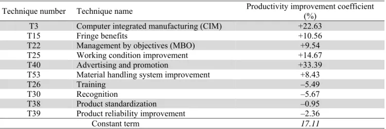
We have also prepared the data file structure based on the computed values of PCt and the collected

data from the factory about the improvement techniques used in the last eight years. With the aid of SPSS package, coefficients A_k can be computed. Table 6 summarizes the results of the candidate techniques.

Applying the proposed model of this paper using the data of candidate techniques yields the following,

max 22.63 T3 + 10.56 T15 + 9.54 T22 + 14.6 T25 + 33.39 T40 + 8.43 T53

subject to:

1.02 T3 + 0.25 T15 + 0.02 T22 + 0.6 T25 + 1.08 T40 + 0.2 T53 ≤ 3 0.9 T3 + 0.03 T15 + 0.05 T22 + 0.2 T25 + 2.5 T40 + 0.2 T53 ≥ 3.5 Tk = {0,1} for k = 3, 15, 22, 25, 40, 53

The optimal solution is T₃∗ =T₁₅∗ =T₂₂* =T₂₅* =T₄₀∗ =1,T₅₃* =0with an objective function of 90.79. A sensitivity analysis using different levels for budget was conducted and results are summarized in Table 7.

Table 6

Productivity improvement coefficients based on a multiple regression analysis

Productivity improvement coefficient (%)

Technique name Technique number

+22.63 Computer integrated manufacturing (CIM)

T3

+10.56 Fringe benefits

T15

+9.54 Management by objectives (MBO)

T22

+14.67 Working condition improvement

T25

+33.39 Advertising and promotion

T40

+8.43 Material handling system improvement

T53

–5.49 Training

T26

–5.67 Recognition

T30

–0.95 Product standardization

T38

–2.36 Product reliability improvement

T39

17.11

(9)

387

Table 7

Optimal selection of productivity improvement. techniques Available budget in million dollars

Solution Objective recommended function

1

T T2 T3 T4 T5 T6

2.8 1 1 1 0 1 1 84.55

2.9 1 1 1 0 1 84.551

3.0 1 1 1 1 1 0 90.79

3.1 1 1 1 1 1 90.790

3.2 1 1 1 1 1 1 98.95

An action plan is proposed and briefly exposed in Tables 8, 9 and 10.

Table 8

Logical framework for the productivity improvement process

Narrative Summary Verifiable Indicators Means of Verification Important Assumptions

Goal: Improving the productivity of Goldi factory

Productivity increases by the next year compared to the current year.

Productivity measurement sheet made at the end of each year.

Purpose: Cost reduction,

profit and demand increase for the factory's products.

Total productivity measures

and indices are improved by the next year.

Demand increases on the

products of the factory.

Productivity measurement

sheet made at the end of each year.

Sales reports.

Management and labor feel and understand the importance of

productivity improvement.

Outputs:

Application of:

Computer integrated

manufacturing (CIM)

Fringe benefits

Management-by-objectives

(MBO)

Working condition

improvement

Advertising& promotion

Positive effect of these techniques on productivity and labor.

Productivity measurement

sheets.

Periodic questionnaires

filled by humans.

Performance reports

presented by departments' heads.

Working laws and

regulations.

Availability of

needed equipment.

Table 9

Project planning matrix (PPM) for application of Computer Integrated Manufacturing (CIM)

1: Level of automation, 2: Actual hours worked/ Total nominal time *100, 3: #annual meetings bet. Mgt. and employees, 4: #employees' complaints about working condition, 5: Sales, 6: #accidents due to material-handling system

CIM1 Fringe

benefits2 MBO

3 Working

condition

improvement4

Advertising and

promotion5

Material-handling system

improvement6

Actual performance % % Million LE

score

10 75 100 19 Zero 550 Zero

9 71 97 18 2 500 3

8 68 95 17 4 450 5

7 65 93 16 6 400 7

6 62 91 15 8 350 9

5 58 89 14 10 300 11

4 54 87 13 12 250 13

3 50 85 12 14 200 15

2 46 83 11 16 150 17

1 42 81 10 18 100 19

0 38 79 9 20 50 21

(10)

Objectives Matrix

Implementation Evaluation Activities Resources (Funding,

people, material)

Department Responsible for Concerned organizations

Important Assumptions

Verifiable indicators (Target)

Means of Verification 1.1 Purchase of a proper

CIM system 1.2 Providing a good

training program for people to use the system 1.3Development of a proper

use and maintenance plan for the system 1.4 Hiring professionals to

ensure that system is running properly and to provide training

Funds from the factory and industry People from the factory and professionals

System is imported; TII Technical;

Education systems is a suggested resource

Electronic production

Deciding system's

requirements

Industrial Modernization Center Customs Authority Tax Authority

System cost is affordable Availability of specialized experts to provide training

Taxes and customs are affordable

The level of automation is increased to about 75%

Performance review reports Financials &

Purchasing

Approving the funds, doing the negotiation and purchasing Training training people to use _{the system} Planning &

Control

Developing plans to make the best use of the system Maintenance Developing effective _{plans to make the best}

use of the system

5. Conclusions

We have presented a mathematical model to choose optimal combinations of productivity techniques. The proposed model of this paper uses linear statistical regression methods to provide the necessary information. The proposed mixed integer programming considers some additional constraints, which are associated with budgeting minimum and maximum limitations. The proposed model of this paper was used for a real-world case study of Egyptian manufacturing company. Based on the results we have determined that different levels of budget may lead to different sets of optimal techniques. Therefore, we can conclude that changes in availabilities or requirements of an organization can change the set of optimal techniques.

References

Aggarwal, S. C. (1979). A study of productivity measures for improving benefit cost ratios of operating

organization. In Proceedings of the 5th conference on Production Research, Amsterdam, the Netherlands,

64-70.

Bellifemine, F., Caire, G., Poggi, A. & Rimassa, G. (2008). JADE: A software framework for developing

multi-agent applications. Lessons learned. Information and Software Technology, 50, 10–21.

Crandall, N. F., & Wooton, L. M. (1978). Development strategies of organizational productivity. California

Management Review, 21(2), 37-46.

Hershauer, J. C., & Ruch, W. A. (1978). A Worker productivity model and its use at Lincoln Electric. Interfaces,

8(3), 80-90.

Huang, S. H., Dismukes, J. P., Shi, J., & Su, Q. (2002). Manufacturing System Modeling for Productivity

Improvement, Journal of Manufacturing Systems. 21(4), pp. 249-59.

Lapin, L. L. (1983). Probability and statistics for modern engineering. Brooks/Cole, Wadsworth, Boston,

Massachusetts.

Masood, T., & Khan, I. (2004). Productivity improvement through computer-integrated manufacturing in post

WTO scenario. InProceedings of the National Conference on Energy Technologies, 171-177.

Nawara, G. M., & Mostafa, M. K. (1991). Productivity Measures and Improvement. Arabic Book, PIEMCO, Cairo,

Egypt.

Rhee, S. K., & Song, I. K. (2000). Productivity improvement of mail delivery: A case study of Korean postal

service. 11th Annual Conference of the Production and Operations Management Society, 1-4 April, 1-3.

Sink, S. (1982). Productivity gain sharing and incentive plans: A current review, Patrick Koeling, D. Scott Sink.

Institute of Industrial Engineers. In proceedings of Fall Industrial Engineering Conference.10 pages.

Stewart, W. T., & Calloway, R. J. (1978). Engineering productivity: The management of improvement.

Engineering Management International, 1, 109-116.

Sumanth, D. J. (1984). Productivity Engineering and Management. McGraw-Hill, New York.

Sumanth, D. J., & Yavuz, F. P. (1983). A formalized approach to select productivity improvement techniques in

organizations. Engineering Management International, 1(4), 259-273.

Sutermeister, R. A. (1976). People and productivity. Thirdedition, New York: McGraw-Hill.

Tsurutani, T. (1990). Manufacturing information systems and productivity improvement activities. In proceedings