Firm financial constraints and the impact of monetary policy: evidence from financial conglomerates

Firm FinanciaI Constraints and the Impact of

ｾＯｬｯｮ･ｴ｡ｲｹ＠

Policy:

Evidence from FinanciaI Conglomerates*

Adam B. Ashcrart Banking Studies

Federal Reserve Bank of ::\e\v York Adam. Ashcraft@ny.frb.org

(212) 720-1617

rvI

urillo Campello Department of Finance 2vIichigan State U niversit.y

campello:Q;bus.msu.edu (517) 3·53-2292

February 12, 2002

Abstract

Building OH recent evidence on the functioning of interna! capital markets in financiaI

con-glomerates, :his paper conducts a novel test of the balance sheet channel of monetary poliey. It does 50 by comparing monetary poliey responses of small banks tbat are afRliated with the same bank holding compan}', and th;.;s arguably face similar eonstraints in aceessing internaije::-.."ternal sources of funds, but that operate in different geographical regions, and thus face different pools of borrowers. Because these subsidiaries typically eoneentrate thei::- lending with smail local businesses, we can use eross-seetional differences in state-Ievel economic indicators at the time of ehanges of monetary policy to study whether or not the strength of borrowers' balance sheets innuence5 the response of bank lending. INe find evidence that rhe negative response of bank loan growtb to a monetary contraction is signi5eantly stronger when borrowers have 'weak balance sheets. Our evidence suggests that the monetar)" amhority 5hou!d consider the amplification effects that financiaI constraints pIay following changes in basic imerest rates and the role of financiaI conglomerates in the transmission o: monetary policy.

JEL Codes: E50, E51, G22. Keywords: monetary polic}", balance sneet cham:el, financiaI conglomerates, internal capital markets.

1

Introduction

Ho\v does monetary poliey arreet the real eeonomy'? The textbook story, often referred to as the

interest rate or money ehannel, is that the Federal Reserve uses open-market operations to enforee

a target for the federal funds rate by managing the aggregate supply of eommereial bank reserves.

The aosence of arbitrage requires that ehanges in poliey interest rates induee similar ehanges in

other short-term interest. rates. In the presenee of stieky prices, these real ehanges in the eost of

capital drive ehanges in the interesr-sensitive eomponents oÍ demando The response oÍ real output

t.o monetary poliey should depend on how far interest rates move and how elastie spending is to

interest rates. In practiee, however, it has oeen ver}" difficult reconeile the observed large and

prolonged output. responses to small and temporary changes in imerest rates, particularly in light

of the ,,·eak evidence of cost oÍ capital erreets on private spending.!

The exeessive sensitivity of output. to monetar)" poliey has prompted ceonomists to look for

a financiaI mechanism - often referred to 2,,8 the credit cha1ll1el - through v;hieh poliey-induced

changes in short-term imeresr rates are greatly amplified. These theories generally emphasize

the importanee of information frietions in ereating financiaI constraints through increases in the

marginal cost of externaI finanee.2 There are two main vie\vs on the credit channel. The lending channel presumes that monetary poliey directly arreets bank loan supply. Draining deposits from banks will reduce lending if banks face financiaI constraints when attempting to smooth these

outnows by issuing uninsured liabilities. \Vhen long-standing relationships provide banks with

infonnation advantage about the quality of their borrowers, firms find the credit orrered by other ｢｡ｊｬｾＱＬＺｳ＠ to be an imperfect substitute. A policy-induced monetary eontractior.. therefore has mueh Iarger erreets on the investmem of bank-dependellt firms than what is implied by the actual change

in interest rates. The balance sheei channel, on the ocher hand, hypothesizes that monetary polic}" arreccs loan demand through its errect on firms' net worth. Higher interest rates increase debt

service and erode firm cash flUlv (or the presem value of ft:ture profits), thereby exacerbating

eonflicts of interest bctween Ienders and high informationj ageney eost borrowers. Higher rates

are also typieally accompanied by declining asset prices, which depress the value of borrowers'

coHateral. This deterioration in firm creditworthiness increases the external finance premiLL"'l:l and squeezes firm demand for credit.

li gTowing number of empírical studies try to assess \vhether 5.nancial constraints Índeed pIay

:See CabaEero (1997) for a sun-ey of the iiterawre on the sensitiviry o: invest:nent to the cost of capital. 2See Hubbard (1994) or Bernanke and Gertler (1995) :or a review of this literature.

ｾ＠

I I

I

ｾ＠

a signifieant role in the transmission meehanism of monetary poliey. Assuming that firm (or bank)

size should be correlated \yith the types of informational frictions that constrain aeeess to eredit markets, most of those studies compare how firms and banks in different size categories change

their investmem (or lending) behavior follO\ying changes in monetary poliey.3 _{unfortunately, one}

important limitation of the existL.'1g research is that it does not distinguish between the role of

financiaI eonstraints in nrrns that would correspond to balance sheet channel and those in banks

that would correspond to the lending channel. Sinee small, nnancially eonstrained nrms are typically

bank-dependent, any observatíon that small nrms are hurt the hardest by a monetary contraction

eannot distinguish between this being driven by a deterioration in nrm credit\vortruness or by

a contraction in the supply of eredit by nnancially constrained ban.ks. Assessing the impaet of

monetary policy purely along the línes of the size of nrms and banks is funher complieated in light

of well-doeumented evidence suggesting that large banks tend to coneentrate their lending with

large firms: one cannot distínguish a differential response of loan demand across firm size from a

differemial response of loan supply across bank size following monetary polie)" shocks.4

The ideal strategy for identifying the lending channel is to look at cross-sectional variation in

COfilllercial banks' ability tO smooth poliey-indueed deposit outfiows holding constant the

charac-teristies of those banks' loan portfolios. Recent research indicates that banks that are affiliated v\-ith

large multi-bank holding companies (BHCs) are effectively 'larger' than their actual size indicates

with respect to the ease in which they smooth Fed-induced deposit outfiows (see Campello (2002) and Ashcraft (2001)). Consistem with Kashyap and Stein's (2000) evidence on the behavior oflarge

banks, those studies show that BHC-affiliate lending is less sensitive to moneta"y contractions than comparable independent banks. This should happen because, differently from independent banks,

members of large BHCs can resort to funds available from conglomerate's internal capital markets

to fund their 10ans even during a Fed tightening. The most straightforward meeharlÍsm tluough

\vhich internaI capitalma"kets work is that holding company could issue uninsured debt on eheaper

3Gert.ler and Gilchríst (1994) and Bernanke, Gertler, and Gilchríst (1996) show that small and large firms nave sígnificantJy dirtercnt investment, growtr., and inventory responses following monetary contraetions. Similar findings are reported by Kashyap. Lamont, and Steín (1994), Olincr and Rudebush (1996), and Gilchrist and Himmelberg (1998;' Lsing data írom banks, Kashyap and Sr.ein (1995. 2000) show that tne lending of large commercial banks is significantly less sensítive to monetary poiicy than that of smal] banks. Thc authors attribute this finding to the ability of large banks to issue uninsured liabilities a,. iow cost (relatívely to smaller banks) when the Fed tíghtens the money suppJy. Kishan and Opiela (2000) observe t.hat the response of lending to monet.ary policy is amplified bO' bank leverage, another measure of fina:1cial constraints.

4Ashcraft (2001) highlights the dirterences in smaE 10an concentration - often used as a proxy for borrower síze _. across bank sizc categories. As of 1996. a typical small ba:->k had 70 perecr.!. of :ts 10an pon.folio composed o;

s:na[ loans (face value of lcss than S 2.50,000), con1pa:-ed to 30 percent fo::: large oanks. Peek and Roser:gren (1997)

terms than the subsidiary bank and then downstream funds to the bank.5 _{InternaI capital markets}

can aIso affeet the ability of the bank to raise extel'nal nnance because o: rhe parem company's

obligation to assist a troubled subsidiary under the Federal Reserve's souree of strength doctrine.

Overall, the evidence from financiaI conglomerates s11O\v t11at bank financiaI consrraints are

impor-:ant in amplifying the effect or monetary policy on bank lending.

On the fiip side, the ideal strategy ror identifying the balance sheet channel is to examine

eross-sectionaI differences

in

Íirrns' financiaI constraints holding constant the characteristics infiuencing

policy-sensitivity oÍ the banks from wbch those firms borrow. This paper builds on the insight that

internal capital markets in BHCs translate into similar nnanciaI constraints for the members of the

same conglomerate to conduct a novel test of the balance sheet channel. It does so by comparing

policy responses of similar size banks that are affiliated with the same BHC but that face different

pooIs of borrowers. \Ve separate these borrowing clienteles by looking at the lending of (same-BHC)

small affiliates that reside in different states. Because these subsidiary banks typically concentrate

their Iending \vith small local businesses whose fortunes are tied to the local economy, it fo11o\\'s

that \ve can use cross-sectional differences in local economic indicators at the time of changes of

monetary policy to study whether borrowers' balance sheet strength infiuence the volume of bank

lending.

Implememing this strategy in bank microdata, we nrst eheek whether there is evidenee

eonsis-tent with signin.eant variations in borrO\vers' balance sheet strength for the banks in our sample.

\Ve do this by looking at the correlation between the business conditions in the localities where

subsidiary banks in our sample reside fu,d the proportion of non-perforning loans they reporto

Us-ing Hodriek-Preseott-n.ltered series on state ineome gap for every US state, we n.nd that differenees

Ín loeal-economic conditions aeross states generate sigl1ifieant differenees in the fraction of

non-performing loans aeross same-BHC subsidiaries of multi-state holding eompanies. \Ve then design

a test of monetary poliey transmission by relating the sensitivity

OI

bank lending to local economic conditions ane the stanee of monetary poliey over a 22-year long period. \Ye n.nd that the nega-tiye response of loan growth to eontraetionary moneta!y poliey for subsidiaries operating during

state-reeessions is mueh stronger than subsidiaries of the same holding eompany that operate in

state-booms. Our results hold for a number of different proxies for the stanee of monetar}' poliey,

and oU! conclusions are robust to cb.anges in the specín.cation of OUI empirical models.

5This could be done either through deposits or by purchasing existing loans rrom the bank, but in either case ,he tra:1sactio:1 would tend to offset t1:!e impact of insured deposit outnows, reducing ar:y need ror t:,e bank to turn to Jarge CDs as a source o: nnance. As:,craft (2001) anc \clayne (1980) show some evide:lce of BHC func char.neEng

along those lines.

[

I

ｾ＠

\Ve design our tests so that usual concerns about the endogeneity of lending/borrowing decisions

and financial constraims are rrjnimized. This contrasts vvith most similar empirical studies, \vllich

have to rely on a series of alL'ciliary tests to address those concerns.6 However, one potential source

of concern for our tests is sample selection. \Ve collect data from banks belongi..'1g to certain types of

financiaI conglomerates to idemify the balance sheet channel of monetary policy. To tlle extent that

financiaI institutions choose to organize their business in particular ways (e.g., choose to operate in various geographical regions at the same), one can argue that OUI data does not come from a

random sample of banks and that our inferences are biased. For instance, a selection bias story

can be argued along the fo11owing lines. Expansionary monetary policies might prompt BHCs to

enter ne\';, fast growing markets (states). If a given BHC based (and restricted to) state A sees an

opportuI1jty to enter the fast grO\ving lending market of state B when access to reserves is easy, it

may change its status from a single-state BHC to a multi-state BHC and thus enter OUI sample,

possibly contaminating our results. \Ve address this and other scenarios in which sampling could

be a source of concem for our empírical strategy in a number of ways. In all cases, we find that

our principal findings on the balance sheet channel remain unchanged.

A cautious interpretation of our filldings would indicate that there is an asymmetry in the

enectiveness of monetary policy over the business cycle 'with policy being more enective when the

economy is in recession than in a boom. As trus asyrrmletry appears to be driven by the

cred-itworthiness of borrm-<:ers, we choose to interpret these findings as consistent with an active and independem balance sheet channel in the transmission mechanism of monetary policy. Such an

interpretatioIl would suggest that when engaging in monetary policy, the central bank should

con-sider the amplification of changes in the federal funds rate on the real economy created by firm-Ievel

fL"'1ancial constraints. Our f..ndi.."'1gs also add to the growing literature on the role internaI capital markets play in the allocation of Íun.ds \vithin conglomerate firms, particularly in financiaI

conglom-erates. Tlis in turn points at need to understand in more detail the innuence of conglomeration

(and merger v.aves) on the impact of Federal Reserve policies OIl bank lending activity.

The remainder of the paper is organized as fo11O\vs. In Section 2, we sketch a simple model

describing the most relevant theoretical questions addressed in the empírical analysis. Section 3

provides a descriptioIl of the data and our sampling cri teria. Our results are presented in Section 4.

6 A gooci example is Kasr.yap and Stei:-. (200C), wno meaSt.:re the monetary palie}" respanses af bank loan-liquidity

sensitivity. The problem is thaT. botr. lending and liquidity management are choice variables to the bank. As the

r

r

I

r

r

I

[

t

A number of robustness checks for om main results are conducted in Section 5. Section 6 concludes

the papeI.

2 Theory

In this section, we analyze a bare bones model that captures the essential elements of the balance

sheet charmel of monetary policy. \Vhile tms is largely an applied paper, we feeI the following

framework is an important contribution to the literature. The existing microfoundations for the

balance sheet channel sketched do not necessarily imply that fum-Ievel financiaI constraims amplífy

the effect of policy-induced changes in short-term interest rates.7 _{To our knowledge, this is the first}

treatmem of nrm-Ievel financiaI constraints which implies that nrm creditwortlüness (measmed by

collateral) necessarily mitigates the response of Iencling to monetary policy.s

We first describe a loan market where private information about the probability of failme creates

adverse selection. vVe then solve for the equilibrium of the model, showing how firms with different

failme probabilities and collateral leveis are allocated between two types of secmed loan markets.

Finally, \ve study how the volume of bank lencling responds to monetar}" policy. Since om later

empirical approach is of a reduced-form that does not rely on estimating structural equations, we do

not hesitate to make simplifying assumptions that facilitate the exposition of OUI main arguments.

2.1

Structure

The representative firm can produce one unit of output at time O, but has to pay its v,orkers' v.ages

w at time O before revenues y are realized at time 1. Firms are endowed with pledgable assets (collateral). Collateral values are either Cl or ch, \vith ch

>

Cl. In this world, workers will not work unless paid in full and production does not take place unless workers contribute with their input.

This problem underlies the fum's demand for credito In the absence of internaI funds, the nrm will

borrow the amount '11.' from a lender (v,:hich we call a bank) at time O with a promise to repay the

amo1L"1t w(l -7 Tb) at time l.

\Ve assume uncertainty over conditions in the product market at time 1. Firm revenues, y,

equal Yh with probability q, and Yl with probability 1-q, where Yh

>

YI. Comracting \vith a lender i8 complicated by the presence of asymmetric information over the probability clistribution of firm

:-evenues across the t,,"o income states. Ir.. particular, we assume that tIle entrepreneur h3S private

7This critique app!ies to the simp!e mode! proposed by Becnanke. Gert!er, and Gilchrist (1996).

8Differently [rom Bernanke and Gert!er (1989) and others of the same genre, our model is not bome ou: a simp!e r:1od:r.cation of the standard IS-L);r fra:ne",ork.

information about this distribution and thus kno\Ys q at time O. The bank, on the other hand, only

has a noisy forecast of q, denoted by E[q:. \Vhen y

<

'U!(1

+

rb) the frm defaults on its loan. In this case, tne bank shuts the firm down and clairns its assets. Otherwise, the nrm repays the loan and

collects the profits. To make the problem interesting, we suppose that the firm always defaults in

the low revenue state. This is consistent with the follmving parameter restriction: (1 -:-rf)

>

ｾＬ＠ \vhere (l

+

r f) is the risk-free rate.

\Ve introduce firm heterogeneity by perrnitting differences not onIy in the value of collateral

firms have, but also in the value of their revenues in the good state Yh. \Ve further suppose that

the probability of the high state, q, takes 011 tv;o values, qh and qz, with qh

>

qz. These 1atter

assumptions are necessary in order for small changes in interest rates to have an effect on the volume of lending.

2.2

Equilibrium

Characterizing the equilibrium conditions in the loan market is complicated by the possibility that firms with collatera1 Ch are ab1e to liquidate some of their pledgable assets and thus look like firms

with collateral

Cz

to lenders.9 _{There are two types of equilibria in the market for bank loans: a}

semi-separating and a pooling equilibrium. \Ve describe the properties of these equilibria in turno

Semi-separating equilibrium. There are two secured loan markets, each differentiated by the leveI of collateral. Firms witil high collateral Ch will choose the type of loan market according to

the probabüity of success q. Those firms witil higher probability of the good state qh will borrow in the \vell-collaterlized loan market. In c011trast, those with smaller probability of the good state

qz \vill ｾｱｵｩ､｡ｴＬ･＠ their pledgable assets and borrow in the less collateralized loan market so long as

the collateral posted Í.:1 the well-collaterlized narket is suHi.cientIy large. Finally, nrms \Vith low

collateral Ci are forced to borrmv in the 1ess collateralized loan market.

In characterizing the serni-separating equilibrium, let us nrst demonstrate that fiTlns ,vith the

high probability of the good state qh and \vith high collateral Ch (henceforth, (qh, Ch)-types) will

choose to bo::-row in the well-collaterlized loan market. Denne

E[qlc]

as the average probability of

the high state given collateral C. A risk-neutral bank witil an opportunity cost equal to the risk-free

rate will price a loall of'U! to the entrepreneur at tile risky interest rate (1 ..;. rb) according to the following pricing ruIe,

9This is motivared by the so-called paradox o: liquidity described in :vleyers and Mjan (1998). \Vhile liqt:id assets

(1 ..;... \ _ (1

+

rf)'W - (1 - E[qic])(YI -:-c)

\- , rb; - E' _{. ,q cw}

I

J . (1)

There is a natural ceiling on this interest rate at

1fZ-:

but it is easy to show that this constraint ,vill not bind unless c is su.fficiently small. Inserting this pricing ruIe into the entrepreneur's net profit

function, condit.ional on the probability q and the leveI of collateral c, yields the fo11O\ving useful expression:

,,(q, c)

=

q(Yh - YI) - E[q ] [(1

+

rf)'W - YI - c] - c.

. q;c (2)

using the fact that E[qlc = Ch] = q;" one can \'-'Tite the difference from borrovling In the

well-collateralized 10an market versus less collateralized loan market as,

\ qh - E[qlc =

czl ( ,

;

7.(q;" Ch; - "(q;,, CI) = .

I

J [\1 -:-rf lu' - YI -

Cz:

>

O.

ｅｾｱ＠ c

=

CI (3)

The inequality fo11ow8 from the parameter restriction ensuring that the nrm defaults in the bac.

state. It follows that (qh, cr,)-types prefer to use their collateral and consequently borrow in the well-collateralized market.

The next step is to ensure that the firm's participation constraint i8 met 50 that 7i( q, c)

2:

O.

This constraint can be written in terms of the value of nrm revenue in the good state,

ｾ＠ (1

+

r f )w - YI - C c Yh

2:

Yh = E[ . •

+

YI - -.

'q,c; q (4)

Xotice that this constraint defines the minimum value of Yh that will be funded by the bank for each

combination of c and q. Imponantly, Yh is increasing in the risk-free rate of interest. Evaluated

at q = qh and c = Ch, 50 that E[q[c = Ch] = %, thi5 equation defines the ,-,olume of lending in the we11-collateralized loan market. Given a cross-sectional distribution G over Yh tb.at is independem of q, aggregate borrowing in the well-collateralized loan market is simply,

L(qh, Ch)

=

u'l:CX;

l(Yh

2:

y'h)dG(Yh). (5) ::\ow let us demonstrate that firrn.s 'with the lower probability or the good state q! will choose to

borrow in the less collateralized loan market. In orde:-to facilitate the algebra, define the ratio or Ch

to Cf as (3, anei rurther define Ctl as the fatio or c, to : (1-;.-r!)w -

yil.

Using these definitions one ca:J.

ｾＭＭＭＭＭＭＭＭＭＭＭＭＭＭＭＭＭＭＭＭＭＭＢＭＭＭＭＭ

-t

(6)

This expression is negative so long as,

L

%" (7)

where we used the fact that 1 - al,3

<

O given (1

+

r f)U' - yz - Ch

>

O. The left-hand side of this

inequality is increasing in the ratio of high to low collateral

f3

as long as 0;/

<

1. It follows that (qi, Ch)-types will prefer to act like firms "ith low collateral Cz as long as the ratio of high to low collateral ,3 is sufficiently large.

The final step is to ensure that the (ql, Ch) type's participation constraint is meto This is done by

evaluating Eq. (4) at q = ql and c

=

Ci, which simply defines the cutoff level of high state revenues

ih

such that the urm chooses to borrow. Firms that are endowed with low leveIs of collateral Cz

borrow in less collateralized loan market, again subject to the participation constraint.

Pooling equilibrium. When ,8 is less than the cutoff value in Eq. (7), there is a pooling equilib-ri um in each the well-collateralized and less collateralized loan markets. As before. entrepreneurs

with the higher probability of the good state will ahvays use their collateral. Using the fact that

E[q!c

=

ChJ = E[qJc = q] we can show that

_ . . __ ( _ _ qh - E[qic

=

Ch]

,·(qn.cnJ ",qh,ez)-CI(3 1) E[q[c= Ch] >0. (8)

This inequality is met since ;3

>

L implying that (qh, Ch)-types choose to use their high leveI of

collateral.

The (q[, Ch)-types, in contrast, wili employ a mixed strateg-y between the two loan markets. The

mixed strateg'Y can be inferred by equalizing the expected returns of borrowing in each or the loan

markets. Followirrg a strategy simila:: to the one above, the equilibrium allocation of this bO!TO\ver

type across the two loan mar kets can be defined by

Ql(3 - 1) _ r 1

1 _{- O;/i.J[q,c} iJ - qZ'E' , _ 1

- Ci;

1 .

- I

E[qc

=

Ch]J' (9)

Recall that the pooling equilibrit:rr: exists when the left-b.and side of this equation is too small

relative to the value or the right-har..d side in the semi-separating equilibrium. The only way

r

[

r

r

,

[

I

r

,

r

•

[

increasing the fraction of (q/, Ch)-types that borro,," in the well-eollateralized market, \vhieh increases

E[qlc

=

q:

and decreases

E[qic =

ｃｨｾＮ＠ l\ote that sinee only a fraction of those with

q

=

q,

choose to

borrO\v in the \yell-eollateralized loan market, it fo11O\vs that the average q in the ,vell-collateralized loan market is largor than that in poorly-eollateralized loan market.

2.3

The Balance Sheet Channel of Monetary PoIicy

Let us now analyze the impact of monetary poliey on the loan market equilibrilLli. \Ve fust study

the semi-separating equilibrium. Recall that firms having both eollateral and a high probability of

the good state borrow in the \vell-collaterlized loan market, where their type is perfeetly revealed

to the bank. The eÍfeet of a ehange in the risk-free rate on the loan interest rate is thus,

8(1 -:.. T_ó)

8(1-;-Tf)

1

(10)

Here an increase in the risk-free rate simply increases the promised payment by the firm, but

since this only occurs in the good state this ehange is scaled by the probability of that state, qh.

Importantly, note that Eq.

(10)

implies that as these firms become riskier or 1ess ereditworthy (i.e.,

qh deereases), their loan rate \ViH have a larger response to monetary policy.

The remaining firms are borrowing in a poorly-collateralized loan market where their type is

not fully revealed to the bank. In this case, the response of the equilibrium 10an rate to an increase

in the risk-free rate is simply,

8(1 -:-Tb) 8(1+Tf)

1

E[qlc

=

q]'

(11)

This expression shows that the response of the loan rate to monetary polic}' will be larger in the

unsecured market so long as borrowers in the secured market have a larger average probability of

the good state.

Looking now the impact of monetary polic)' on loan interest under the pooling equilibrium,

recall that the ave' age probability or the good state is larger in the \yell-collateralized loan market

than. in :he unseeured loan rnarket. This suggests that monetary polie}' has a larger eÍfect Oil the

loan rate of unseeured borrowers. Note also that there is an additional eÍfect working in the same

direetion: an increase in the risk-free rate also increases losses in default states, implying there is

an dee:-ease in 0:1. Since the left-hand side of Eq. (9) is incre2.sing in 0:1, tnis requires an adjustment

in lhe fraetion of low probability types that choose to borrow in the well-eollateralized loan market.

A reduetion in 0:1 reduces tb.e left-hand side of Eq. (9), implying that ,ve must nnd a way to reduce

t

l

t

t

r

t

ｾ＠

l

ｾ＠

I

l

the right-hand side of this eqllation. As before, this is only accomplished by a larger fraction of

low probability f..rms shifting from the secured to ll1lsecured loan market, an effect that amplines

the effect of monetary policy on llnsecllred borrowing.

It is no\v a straightforward task to eva111ate how monetary policy affects the volume of lending in our modelo First, reconsider the participation constraint in Eq. (4). Ir ShOllld be clear that an

increase in the risk-free rate increases the 10w8:" bound on Yh, which implies that the volume of

lending will decrease. At the same time, note that the response of lending is proportional to E[;lcj'

implying that the volume will fall by more in response to a monetary contraction in markets where

E[q!c]

is smaller. Recall that both the pooling and sewj-separating equilibria had the property that

the well-collateralized 10an market had a larger

E[ql<.

This implies that collateral tends to mitigate

the response of lending to interest rates. In orher words, the equilibrium of OUI model predicts that

borrowers' creditworthiness will infl.uence the response of bank lending volume to monetary policy

shocks precisely along the of t11e balance sheet channel: higher basic interest rates will reduce the

borrowings of a11 nrms, but will affect those nrms with low collateral values particularly more.

In the empirical investigation that follows we focus on borrowers for which the implications

of information-based theories nt well \vith the observed structure of n.nancing arrangements. In

particular, we examine the relationship of nmulcial intermediaries with borrowers that are likely

to characterize the entrepreneur \vith a single idiosyncratic project and whose business demands intensive monitoring. These are prL.'1J.arily small nrms and individuaIs. l\lost of the small nrm nnancing in t11e

0.5.

is intermediated, v .. ith the majority of the credit being provided by commercial banks. Note also that the use of eollateral, eovenants, and other guarant.ees are present in nearly all

. of the financing contraets between banks and small nrms and individuaIs. Similarly to Bernanke,

Gertler, and Gi1christ (1996), we argue that examining data on bank loans geared towards thjs type

of borrO\vers wiU provide for the best way to identify t11e workings of the balance sheet channel in

practice.

Before we conclude let us emphasize the importance oÍ the role L.-nperfect information

(alterna-tively, high agency costs) plays in the transmission mechanisEl by considering the response of the

10an rate and volume to monetary poliey across the amount of collateral in the absence of private

information about

q.

This v,'-ould imply that

E:qJc]

=

q,

which means t.hat 10ans are priced in a

manner such that nrm payons are independem oÍ coEateral. Rewriting Eq. (2),

In ｾｨｩｳ＠ \yorld, eacn firm is indifferent between borrowing in either loan market, so there should

be no equilibrium correlation betv,een the amount of collateral and probability of tne good state.

It follows that as the cutoff value yj, no longer depends on the amount of collateral, there are no

longer differential enects of loan volume to moneta:-y policy across c. It follows that a useful test

OI the importance of financiaI cOllstraints in the transmission mechanism is to consider whether or

not the response of lending to monetary policy is mitigated by the value of collateral.

3

Sampling Methodology

In order to identify the response of a loan demand to monetary policy it is necessary to eliminare any dinerences in fiIlancial constraints across banks that would drive a differential policy-response

of loan supply. Such an anaIysis requires one to use banks that face similar financiaI constraints,

but experience differential strength in their borrowers' balance sheets. Our study uses such a

strategy to look for evidence on the balance sheet chamlel of monetary policy. Here we describe

the identification problem and our approach in detail, and tnen discuss the data employed.

3.1

Identification

\Ve model the differential response of bank lending to monetary policy across banks by explicitly separating demand and suppIy-side effects of monetary policy. Let rt denote the stance of monetary

policy as of time

t,

Eq. (13) writes the response of loan growth to policy for an individual bank i

that is part of holding company j at time t,

(13)

Differences in the response of loan demand across banks are captured by Aijt and Bijt , wb.ich correspond to balance sheet and non-balance sheet enects, respectively. The first of these demand

enects can be understood in the spirit of our 1110del, whe::-e the demand for loans by firms with poor

balance sheets and límited collateral will decline following a monetary contraction. The second

Tefers to óanges in [oan demand that are not related to fim:. financiaI strength. Firms involved

in the manufacture of durable goods, for example, have product demand that is more sensitive to

monetar}" polic}" tha:J. other firms. One should thus expect to see relatively more policy-sensitive

lending by banks that concemrate their business \\'ith these D.rms. Differences in the response of

loan supply across banks are caused by differences ir.. tlle severi:y o: financiaI constraims they face

t

r

r

ｾ＠

I

t

[

at the bank-le\"el, ｘｬｪｾｮｫＬ＠ or the holding company-level,

xHf

C .lO These controls are meant to capture leuding channel effects where fimmcial constraints affect the abilíty o: banks to replace an outRow of insured deposits with other funds.

Given the appropriate data on each of these regressors, estimating Eq. (13) via Ordinary Least

8quares would recover the correlation of firm balance sheet strength with the response of bank

Iending to monetary policy through the estimate of 0:1. The problem with this strategy, however, is lack o: data on a11 of the relevant dimensions of each of these regressors. lu particular, there

are likely to be unobserved components of B ijt , Xllínk , or XHtHC that are correlated with the observed dimensions of firm balance sheet strength Aijt , in which case the OL8 estimation v;;ill be

compromised by omitted variables bias.

\Ve attempt to minimize trus problem using several devices. First, we restrict our sample to

banks that are affiliated with large multi-bank holding comparues. T}lis Íollows Írom the evidence ou

recent research on the bank lending channel. Kashyap and SteÍll (2000) show that Iarge commercial

banks are mostly insensitive to monetar}' policy shocks, as their ability to tap ou uon-reservable

sources oÍ funds at lo\\' cost allows them to srueId their leuding from Fed-induced contractions.

Campello (2002) and Asheraft (2001) further demonstrate that, just like Iarge ban..1cs, subsidiaries

oÍlarge BHCs are far less constrained than comparable independent banks. Based on these findings,

that sample restriction aloue should all but eliminate the importanee of bank (supply-side) financiaI

constraints in expIaining the response of lending to monetary policy, allowing us to disregard ｸｴｾｮｫ＠

and X_i

1f

C . \Ve, however, weaken such an assumption and estimate Eq. (13) inc1uding a set of Xijt

variables that, according to the Iending channelliterature, should e.,'(haust the sourees of v-ariation in

bank-level financiai constraints: capitalization, size, and liquidity. In the end, 0:3 and 0:4 should be

very sma] - if not zero - so that even if there are unobserved dimensions of bank/BHC financiai

constraints, any correlation of these unobservables with firm balance sheet strength ís mitigared. E

The second device we empIoy to mitigate omitted variables bias is to foeus the analysis on

the differer.ce between a subsidiary's response to monetary policy and the average response o:

｡ｾｬ＠ of the other ban..1cs affiliated with the same holding company. Focusing on within-conglomerate comparison8 is u8efu1 because it eliminates financiai eonstraints at the BHC-leveI from the equation,

purging Ol1e potentia1 source of bias. Define

Dijt

as the difference betweeu a subsidiary's Xijt and

lODependence on holding company-level financiaI heai7,h is bduced by regulation requiring that financiaI conglom-erates r:1\:st operate on consolidated basis. See Houston, James. and ::'vlarcus (199í) for a discussion.

r

r

ｾ＠

i

r

r

,

r

r

[

t

its holding company mean in a given quarter. We can re-write Eq.

(13)

in differences from the holding company mean as fo11o\','s,

(14)

Once we have minirnized bank-driven differences in loan-policy responses, the next device ,ve

use to reduce the influence oÍ biases is to isolate sources of cross-sectional variations in borrower

balance 5heet strength which are presumably uncorrelated with the other ornitted variables. \Ve

lack data on every borrower of every bank in our sample oÍ BHC subsidiaries. :Nonetheless, \,\'e have

a rich dataset describing the markets (or local business conditions) where 10an5 are made. Arguably,

depressed economic activity within a state wiH lead to a deterioration in local borrowers' balance

sheets, as small, local businesses fortunes (cash fiows, collateral values, etc.) are intrinsically tied

to the local economy. Our identification scheme is complete if we can assume that these borrowers

concentrate most of their lending with small banks.12 _{'vVe thus isolate differences in borrowers'}

strength across members of a given conglomerate (Q&t) by looking ar data from small subsidiaries

of large multi-state conglomerates.

Our approach is sound if we isolate from A ijt those unobserved components that are likely to

be correlated with Bíjt . This is 110t a11 obvious task. The solution involves the observation that

variations in Aijt can be broken out into both high-frequency and low-frequency components. The

low frequency component is potentially correlated with Bijt .:3 The high-frequency component of

Aijt, on the other hand, is plausibly independent of non-balance sheet Íactors. In implementing

our tests, we exploit the high-frequency variation in firm balance sheets that is induced by

short-run changes local business conditions. In essence, our identifying assumption is that short-term

deyiations fram long-run econornic trends at the state leyel are uncorrelated with non-balance

sheet driyers of the response of bank lending to monetary policy, Bijt , and unobserved measures of

bank-level financial constraints, _, X,bJ;n". _J'

1ZSuch an ｡ｳｳｵｭｰｾｩｯｮ＠ is strong!y supported by ext,ensive research on business lending practices of small and large banks. See, among others, :\"akamura (1994), Strahan and Weston (1998), Berger, Saunders, Scalise and Udell (1998), di Pat:i and Gobbi (200:), and Sapienza (2002).

13RecaIl, Bijt crives differences in thc response of loan demand to monetary policy that are not created by borrower

financiaI constraints, but by underlying characteristics of the borrowers in a market (or state), such as the sensitivity o: product demand to monetary policy. lt seems plausible to t,hink tna: such characteristics (e.g" industrial stn:cture) evolves quite slowly ove:: time and are essentially fixed over short periods of time.

3.2

Data

\Ve collect quarterly accounting information 011 tÍle population of insured commercial banks from

the Federal Reserve's Call Repori of Income and Condition over the 1976:I-1998:II períod, using a version of the data that was cleaned by the Banking Studies Function of the Federal Reserve. After

a inibal screening, we retain only bank-quarters with positive vaIues for total assets, total Ioans,

and deposits. Details about the cons:ruction of the panel data set and formation of consistent time series are provided in Appelldix A.14

The single most important bank-Ievel variable used in our anaIysis is loan grov:th. This variable

is defined as the quarterly time series difference in the log oÍ totalloans. \Ve use the bank merger file

published online by the Federal Reserve Bank oÍ Chicago to remove any quarter in which the bank

makes an acquisition, which helps reducing data measurement problems with the differenced data.

In addition, we eliminate any quarter in which bank Ioan growth is more than 5 standard deviations

from the mean in absolute value. Since the regressions below include four lags of loan growth as

explanatory variables, the sample is implicitly liwjted to banks having ai least five consecutive

quarters of data. The first five quarters of the data are Iost in order to construct lagged dependent va,riables and appropriate differences.

Our analysis focuses on the Iending of small banks. This sampIe restriction is made in order to

best match the state in which the bank is chartered with local business conditions.15 _Consistent

with previous studies, we define as 'smal!' banks those bank-quarters in the bottom 95th _percentile

of the assets s1ze distribution of a11 observations in a given quarter.16 _{There are 926,845 small}

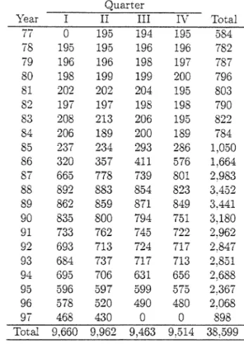
bank-quarters contained in the 1977:II-1998:II period. The first restriction we impose on the data

1S to retaill only small banks that are part oÍ multi-bank holding companies which control at least

one large bank (i.e., a bank in the top 5th percemile of the asset distribution). This d:ops the number of bank-quarters dmvn to 94,333. ::\ext, we require that small banks must be afD.Iiated

witi: holding companies that have subsidiaries residing in at least two differem CS. states during

the same quarter. These restrictions leave 38,599 bank-quarters in our panel dataset. The time

distribution of the number of observations in th.i.s 'raw' sample of multi-state BHC subsidiaries

is reported in Table 1. The table shows a stead:y increase in the number of observations in each

quarte:- untE the advent of problems in the bankirlg industry in the late 1980s. During the last

'4Program code is available fro:n the ｡ｵｾｨｯｲｳ＠ upon request,.

15 A large bar...k 's loa:l oP?ortunities is probabl,y poorly measurec. tl:e economic conditions of the s"Cate in l-Nhich it

is d:arterec..

decade, consolidation \vithin the industry (and wi;;hin BHCs) has greatly reduced the nUillber of

small banks affiliated with large BHCs to currently approximately one-third o: its peak number in

1988Y

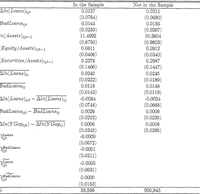
The firse column of Table 2 reports the mean and standard deviatio:l of the variables used

111 our analysis. The statistics in the first coIUJ.1'""l. of the tab1e are for the small banks that are

included in the samp1e. The figures for basic balance sheet information such as size, 10an growth,

leverage, etc. are similar to those reported in similar studies on small banks (see, e.g., Campello

(2002)). Banks in our final sample display a quarterly 10an growth average of 1..57 percent \vith a

standard deviation of 7.6 percent. Xote that the standard deviation of 10ng-run 10an growth and

non-perfornüng 10ans are similar in magnitude to the 10ng run means, implying that there are large

differences across banks in long-run average loan growth and non-perrorming loans.

As we discuss below, we must be concerned with the fact that OUI data selection criteria may

create samp1e biases that affect our inferences. To check whether the observations in our samp1e are

"u.'1ique" in some obvious sense, we also compute descriptive statistics for the variables of interest

using those small banks that are left out of OUI final samp1e. Comparisons based on those statistics

suggest that one would have a difficult time arguing that small subsidiaries of multi-state BHCs

operate very differently from other banks in the same size category.

Finally, OUI analysis also necessitates data on the stanee of monetary poliey and on the business

environment in \Vhieh the small affiliate banks in our sample operate. The measures of monetary

policy \ve use are fairly standard and are described in detail in Appendi'\: B. :\Iost of these poliey

measures are eOllstructed y,ith series availab1e online from FRED at the Federal Reserve Bank of

St. Louis. In order to measure local business eonditions we use the nominal state ineome series

av-aílable online from the Bureau of Economie Analysis. Deviations from the long-run eeollomÍe

growth trelld in eaeh state are used to charaeterize state-reeessions and state-booms. Specífically,

a state 'income gap' (YGap) 15 construeted by applying an Hodrick-Prescon frIter (bandwidth of

1600) to the time series difference of the log of total state income for each state anei the District of

Columbia.

"\\"ithom weignting t hese trends in r,he number of obsen'ations, statistics constructed on this sample would place an unusual amount of weight on toe first decade of data. As the analysis below is done quarter bO' quarter, this wil! not be a concern. but ,he descriptive statisdcs dLsplaO'ed in Table 2 would inherit this property.

t

i

[

,

t

r

l

4 Empirical Results

4.1 Local Busi.ness Conditions and Bad Loans

In order to substantiate our testing strategy we need to find evidence that depressed economic

acti\"ity actually depresses borrowers' balance sheets. To our knowledge, there are not public

ayailable data on individual firms' borrowings that serye our purposes. On the other hand, we

do have data on the loan portfolio of their banks. In establismng a link between local economic

conditions and fum balance sheets, we argue that an unexpected deterioration in firm balance sheets

should show up in the quality thei! banks' loan portfolio. We examine this working hypothesis in

turno

For each individual bank i affiliated with the holding company j at time

t,

let

nf)t

denote the difference bet\veen a subsidiary's bad loans (i.e., non-performing loans) and the average bad loans of

all other small banks in the holding company. Similarly, define

n;;f

AP _{as the difference between a}

subsidiary's state income gap and the average income gap of all small banks in the holding company,

oBadLoans B dI B dI

" "ijt = . a ·oanSijt - a oansjt, (15)

(16)

The issue of interest is whether subsidiaries operating in state-quarters with relatively poor

economic conditions report a greater fraction of loans gone bad. \Ve use the following empirical

model to address this question:

4:

013adLoans _ ..L ' \ " ' \ "YGap..L 0)( ..;.. '\"' 1 . . L : ..

"",)t - ri ' L...-AkHijt_k ' --,)t-k . L...-at t , ｾＧｊｴﾷ＠ (17)

k=l

The set of controls included L'1 X is composed of lagged of log assets, the lagged bank equity ratio,

and the lag of bank liquid assets. The a coefficients absorb time-fixed effects. The four lags of log

b . h l ' BHC' 10vGav' . t ' l ' .

c .auges lJ1 t e Te atlve-to- state mcome gap

,--ijt

.)

are meant to cap ure tne re atlve strength

of the balance sheets of the borrowers of the subsidiary bank. \Ve are, of course, interested in the

relationship between a small subsidiary's (relatíve-to-BHC) ratio of bad loans and the financiaI

status of the businesses in its market, captured by

L:

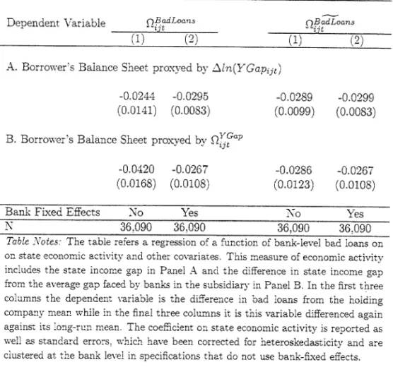
À.

Vv·e report the estimates returned for

L:

À 1.'1 Table 3 (standard errors are corrected for clustering

and heteroskedasticity). Pane: A simply uses the state income gap !:::.Zn(YGapijr), whiIe Panel B

uses

fl,:?a

_'J" p. T!J.ese pooled cross-section times series regressions are estimated both witl, and without

ＮＭＭｾｾｾｾｾｾｾｾＭＭｾｾｾｾｾｾｾｾＮ＠ _ _ . _ - - -

-t

r

the state income gap by one stanàarà àeviation oÍ the income gap (about 2.4 percentage points)

reàuces the fraction of bad loans in a small bank's loan portfolio by about 6 to 10 basis points.

\Vhile these effects are statistically significant, this may seem like a relati\Oely small deterioration

i:c. bank loan credit quality, representing less than 10 percent of the sample mean. :\"otice, however,

that bis estimate represents the impact of a slowdown in state income on bad loans in the current

quarter, and that the curnulative deterioration in firm credit quality could be several times as large

over a longer time horizon.

One potentiallirnitation with this specification is that it exploits both permanent and transitory

differences in the fraction of bad loans across subsidiaries. In principIe, we are interested in bad

Ioans created by what are temporary changes in local econornic conditions, so it makes sense to

elirninate long-run individual bank effects. This can be accomplished by differencing out any

bank-Ievellong-run differences reIative to the holding company, defining DgfdLoans as fo11ows:

ｯｊＳＮｾ｡ｮｳ＠ = oJ3.adLoans _ "BadLoans

"'Jt '-'Jt ｾ＠ "J (18)

\Ve re-exanüne the question of relative loan performance, nO\v only exploiting transitory

differ-ences in bad loans across subsidiaries, by estimating the following equation:

4

ｏｂｾ｡ｮｳ＠

+ "" \

OYGap , j3"X -L " " 1 '

-'"ijt

=

7] L... Ak'"i.jt_k T Hijt' L... at t T C.ijt· (19)

k=: t

The resuIts from this last estimation are reporteà in Table 3. The fust panel uses state income

gap while the second uses the equiv-aIent relative-t.o-BHC measure Ｈｄｾｾ｡ｰＩＮ＠ There continues to

exist clear evidence that differences in the state income gap drive temporary differences in bad

loans across bank subsidiaries. \Ve interpret these resuIts as motivating evidence for using the state

income gap as a proxy for borrower credit.\vorthiness.

4.2 Local Business Conditions and Asymmetric J\1onetary Policy Effects

\Ve have established that cross-sectional differences in economic conditions of the \-arious markets

in which a conglomerate operate drive differences in tne loan quality (indicative of borrowers'

financiaI strength) among the various subsidiaries of the same conglomerate. \Ve now turn to the

main question of the paper: \Yhether there's a balance sheet channel of monetary policy.

To investigate this transmission mechanism we use a two-step approach 'which resemhles t.hat

of E:ashyap and Stein (2000). The idea is to relate the sensitivity of bank lending to local economic

conditions and the stance of monetary policy by combining cross-sectional and times series

regres-sions. The approach sacrifices estimation efficiency, but reduces the likelihood of Type I inference

errors - i.e .. it reduces the odds of concluding that borrowers' finances matter when they really do nOL 1S

Define nMans as the difference between subsidiary lending and the average loan growth of all

other small banks in the conglomerate. The first step of our procedure consists of ru:ming the

following cross-sectional regression for every quarter t in the sample:

(20)

To explicitly account

ror

the idiosyncractic long-run effects discussed above, we also estimate the following ;double-differenced' equation:

_ 4 ｾ｟＠ 4 _ ｾ｟＠

r.Loans _ . ｾ＠ r.Loans· ｾ＠ N OYGap '(3r.X ,

Hij - 7) -:-L...t 'iTkHijt_k - L...t fk""ijt-k'" H i j - l " Eij, (21)

k=1 k=l

From each sequence of cross-sectional regressions, we collect the coefficients returned for

2:::

ｾＨ＠ and 'stack' them into the vector Wt, which is then used in the following (second stage) time series regression: 19

8 8 3

Wt =0:";" L0k JfPt-k, LJ.LkD.Zn(GDP)t-k";" I:>·kQk..;..pt-:-l1.t. (22)

k=: k=l k=l

Of course, we are interested in gauging the i1l..fl.uence of monetary policy, 111 P, on the sensitivity

of loan growth to borrower balance sheet strength. The economic and the statistical significance

of tLe impact of monetary policy in Ec;,. (22) can be gauged from the sum of the coe:ncients for

the eight lags of the monetary policy measure

(2:::

ó) and from the p-value of this sumo Because polic}' changes and other macroeconomic movemems often overlap, we must d:stinguish between

:8An alternative one-step speciflcatiol1 - wit}:). Eq. (22) below nesteci in Eq. (20) - would impose a more constrained parametrization and }:).ave more powe:- to reject lhe null }:).ypothesis of borrowers fir:ances irrelevance. However, test.s of coerncient stability indicate that t.he data strongly rejects those parameter restrictions. Another advantage of t}:).e tW0-step approach h< that it allows for cross-sectional variations in local dernar:d conditions to be accoum.ed for in e\'ery pe:-iod.

19To see how t}:).is procedure account.s for the error conta;ned in the flrst-step, assume that the true \V; equals what is estimated from the first-step run (\Vt) plus some residual (li,):

W;

= \Vt

+

li,. One would like to estimate Equation (22) as 'li; = '" -'-

xe

+

"'t,

"'11ere the error term would only refiec: the errors associated wit,h the speci5.cation of the moce:. However, t}:).e empírical version of Equation (22) uses \Vt (rather than \Vn on the right har:d-side. Conseqaem.ly. so long as E [X'v: = O, '" wil! absorb the me ar: of VI, while 'Ut wEl be a mi.'G:t:re of Vt ar.d Wt. That

is. lhe measaremer:t errors of r.he first-step \Vil] increase t}:).e tot.al error \'ariance in '.he seconà-step. but wiIi not bias

r

,

r

J

I

J

r

r

financiaI and real explanations for the observed relationship between bank lending and borrower

st;:ength. To check whether the measure of monetary policy retains signincant predictive power

after conditioning on macroeconomic factors we include eight Iags of the Iog change in real GDP in

the specification. The variable

Q

corresponds to quarter dumn:jes, and t represellts a time trend.

Since there is lir.tle consensus on the most appropriate measure or the stance of monetary

policy we use four alternative measures in ali estimations performed: a) Úle Fed funds rate (Fed

Funds): b) the spread betv,een the Fed funds rate and the rate paid on 10-year Treasury bills

(Funds-Bill); c) the spread betvveen the rates paid on six-month prime rated commercial paper

and I80-day Treasury bills (CP-Bill); and d) Strongin's (199-5) measure or unamicipated shocks to

reserves (StrongL'1). All monetary policy measures are transformed so that increases in their leveIs

represent Fed tightenings.

Figure 1 pIots the empírical distribution of the coeflicient of interest from the first stage

regres-sions,

I:

T This empirical distribution is constructed using a kernel density estimator, which is essentially a non-parametric estimator ror a continuous probability distribution. \Ve perform the

first stage estimations of our two-step procedure in four different ways (see below), yielding a total

of 364 realizations. As expected, those estimations return a positive coeflicient for

I:

i in most runs. The mean (median) of those coefficients equals 0.078 (0.027) and is statisticaliy different from

zero at the 0.1 (0.1) percem 1eve1.2_{o A positive coeflicient indicates that there is more demand for}

credit by firms in states where business c6nditions are favorable and Ullconstrained banks are abIe

to provide financing. Of course, these univariate results alone don't say mude. about the dynamics

of the transmission of monetary poli c}'.

The main results of the papeI are reported in Table 4. The table reports the sum of the

coefficients for the eight lags of the monetary policy measure

(I:

ó) from Eq. (22), along with the p-values for the sun1. Heteroskedasticity- and autocorrelation-consistem errors are computed with

::\ewey-vVest lag windo,," of size eight in all regressions. The table sUIIl.I:larizes the results of 16

two-step estirnations (four different Erst stage regressioIls x fOUI monetary policy measures). The

results in Panel A use the state income gap 6.lnCY" Gapijt) as the proxy for local borrowers' financial

status, \v}:1jle those i:l Panel B use ｮｾＷ｡ｰ＠ (the difference between the income gap facing a subsidiary and the average gap facing all other small subsidiaries of the same BHC) as the relevam proxy.

The nrst ro\\" of each panel reports results from regressions that use

nMans

(the relative-to-BHC

subsidiar)" loan growth) as the dependem yariable (see Eq.(20)), while those in the second row use

20I\otice tnat we are not claiming that the ＧｾＧＭｲＧ＠ realizations are indcpenden:: across rU:1s.

t

r

t

t

r

r

r

,

r

r

r

r

f2D'tans (the double-differenced f2Mans) as the dependent variable (Eq. (21)).

All of the coernciems in the table have the expecred sign, and most measures of lr..onetary polic)"

return statistically significam coerncients. This is rema:ckable given well-documemed dirrerences

in the time series properties of policy measures based on the interest rates and those based on

monetary aggregates. Of these coernciems, twelve (seyen) are significant ar the 9.6 (3.9) percent

level or better. The coerncients for the most conventional measure, the federal funds rate, are all

significant at better than the 6.5 percent level.

In order to interpret the economic significance of those estimates, it is necessary to select a

baseline policy experimento Consider the scenario in which the central bank increases the funds

rate by 25 basis points and keeps it there for eight quarters, implying a 200 basis point change

over the entire horizon. Using the most conservative of our fed funds rate estimates (0.031), a

one standard deviation deterioration in the state income gap (0.025) faced by a subsidiary \vould

amplify the impact of this monetary contraction on bank loan grov,1:h by some 15 basis points

in the current quarter alone. To see what this result would imply in dollar terms, consider two

subsidiaries of the same EHC, both with a loan portfolio equal to 8100 million (about the average

figure for banks in our sample as of 1998:II). Suppose one of the subsidiaries operates in a state

where the income gap is one standard deviation above average and the other operates in a state

\vhere the ｩｮ｣ｯｭｾ＠ gap is one standard deviation below average. Then a 25 basis point increase in

the fed fU.11ds rate sustained over eight quarters would lead the loan portfolio of the bank facing

a local slump to cut back on lending by 8300,000 more in the currem quarter than the first bank

facing a local boom.

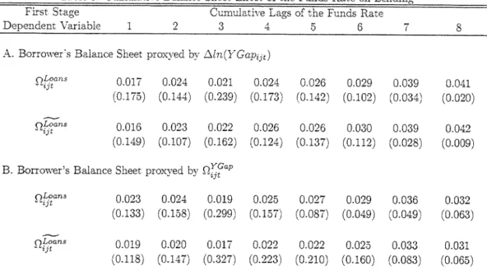
Table .5 illustrates the complete 'impulse-response' of balance sheet amplífication using the

federal Iunds rate as a measure of monetary policy. The rows OI the table are similar to the previous

tabIe, \vhíle tne columns correspond to the point estimate and p-value for sum of coeffi.cients across Iags of the funes rate. The time pattern describes an initial errect of 1.5 to 2 percent on the currem

quarter bat increases to 3 to ｾ＠ percent after eight quarters. These estimates imply tnat the bulk

of the amplification errects implied by tne balance sheet channel of monetary policy takes place

immediately arter a policy change. They also shmv that the errects of monetary policy on bank

lending that are induced by borrowers' financiaI \veakening is very persistent through time. Tne

timing and duration of balance sheet errects ove,: the business cycle \ve unco;;er are roughly similar to

those Gertler and Gilchrist (1994) find using aggregate times series data rIOm small manufacturing

nnns. These patterns suggest that the presence of firm-level financiaI constraints could help explain

20

the excessive sensitivity of output to short-term interest rates. Moreover, in the presence of a strong

balance sheet channel there are importam asymmetries in the transmission mecnanism of monetar}"

policy o\·er the business cycle that need to be acknowledged both in forecasting futUIe econorn.:c

performance and in the design of poli c}".

The analysis of this section established that there are important differences L'1 the response of

bank loan growth to monetary policy over the state business cycle. vVe want rely on the evidence

that movements in the state econornic conditions are correlated with movements in the

credit-worthiness of local borrowers in order to interpret OUI findings as consistent with a balance sheet

channel of monetary policy. Berore we conclude, hO\vever, we discuss some potential weaknesses

with the eyidence above.

5

Robustness

Although we use an approach that resembles that ofKashyap and Stein's (2000) two-step procedure,

OUI analysis is far less subject to the simultaneity biases discussed in their papeI. Specifically, whi1e

OUI second-stage times series regressions are similar to those of Kashyap and Stein, their paper's

first-stage regressions involve estimating the sensitivity of a bank's choice variable (lending) to

another endogenous variable (liquidity). OUI first-stage regressions, in contrast, involves estimating the sensitivity of loan growth to local economic conditions, which are exogenous to the bank's decision set. This relieves us from having to consider whether OUI results could be explained away

under v-arious scenarios in which banks may choose to behave in a specific way (say, they may hold

more liquid assets) when they know their borrowers to be particularly sensitive to monetary policy

or business cycles. Our approach, on the other hand, is subject to different types of criticisms.

5.1

Sample Selection: Heckman Correction

One potemial SOUIce of concern for OUI tests is sample selection. In particular, we select rrom

the popuiation of insured commercial banks only those small banks belonging to cenain types 01

financiaI conglomerates. To the extent that financiai institutions choose to organize their business as multi-bani:: firms and ma}' decide whether OI not to operate in v-arious geographical regions, one

could argue that OUI data does not come from a random sample of banks. If this sample OI ｢｡ｲｾＱＨｳ＠

was constant over the complete time period. this would not be a problem as inÍerence could sir::J.ply

be dOlle conditional on the sample. The potemial selection probiem is that the sample changes in

non-random ways ove:- time as bank holding companies acquire other insütutions a:r..d consolidate