Enhanced incoherent scatter plasma lines

(1)

Enhanced incoherent scatter plasma lines

H. Nilsson1, S. Kirkwood1, J. Lilensten2, M. Galand2

1Swedish Institute of Space Physics, Box 812, S-981 28 Kiruna, Sweden

2Centre d’Etudes des Phenome`nes Ale´atoires et Ge´ophysiques—ENSIEG, St Martin d’Heres Cedex, France Received: 1 December 1995/Revised: 19 April 1996/Accepted: 25 April 1996

Abstract. Detailed model calculations of auroral second-ary and photoelectron distributions for varying conditions have been used to calculate the theoretical enhancement of incoherent scatter plasma lines. These calculations are compared with EISCAT UHF radar measurements of enhanced plasma lines from both the E and F regions, and published EISCAT VHF radar measurements. The agreement between the calculated and observed plasma line enhancements is good. The enhance-ment from the superthermal distribution can explain even the very strong enhancements observed in the auroral E region during aurora, as previously shown by Kirk-woodet al. The model calculations are used to predict the range of conditions when enhanced plasma lines will be seen with the existing high-latitude incoherent scatter radars, including the new EISCAT Svalbard radar. It is found that the detailed structure, i.e. the gradients in the suprathermal distribution, are most important for the plasma line enhancement. The level of superthermal flux affects the enhancement only in the region of low phase energy where the number of thermal electrons is compara-ble to the number of suprathermal electrons and in the region of high phase energy where the suprathermal fluxes fall to such low levels that their effect becomes small compared to the collision term. To facilitate the use of the predictions for the different radars, the expected signal-to-noise ratios (SNRs) for typical plasma line enhance-ments have been calculated. It is found that the high-frequency radars (Søndre Strømfjord, EISCAT UHF) should observe the highest SNR, but only for rather high plasma frequencies. The VHF radars (EISCAT VHF and Svalbard) will detect enhanced plasma lines over a wider range of frequencies, but with lower SNR.

1 Introduction

The plasma line is a well known, but little used component of the incoherent scatter radar spectrum. It is a signal scattered from high-frequency electron waves, Langmuir

Correspondence to: H. Nilsson

waves. Two plasma lines can be detected by the radar, one upshifted from the transmitted frequency, and one shifted. These lines correspond to scattering from down-going and updown-going Langmuir waves respectively. The frequency shift from the transmitted signal is the fre-quency of the scattering Langmuir wave plus the Doppler shift caused by the bulk motion of the electron gas. The wave vector of the scattering Langmuir wave is deter-mined by wave vector matching requirements with the incident and reflected electromagnetic waves. The re-flected waves are shifted in frequency, and the up and downshifted plasma lines will have slightly different wave vectors. In practice this difference in wave vectors leads to significant differences in offset frequency and if the Dop-pler shift is to be measured the dispersion relation of the Langmuir waves must be known with good accuracy (e.g. Hagfors and Lehtinen, 1981; Heinselman and Vickrey, 1992; Kofmanet al., 1993). The frequency of the Langmuir wave is close to the plasma frequency, i.e. a few MHz for most realistic conditions. The wave number dependence of the Langmuir wave dispersion is primarily dependent on the electron temperature.

(2)

collisions will damp the Langmuir waves toward their thermal level (e.g. Yngvesson and Perkins, 1968).

Plasma lines have a number of potential uses: the system constant for the incoherent scatter radar can be determined with good accuracy using plasma frequency measurements, e.g. Kirkwoodet al., 1986. Such measure-ments can also be used to determine the electron temper-ature independently of the ion line analysis (Hagfors and Lehtinen, 1981; Kirkwood and Bjørnat, 1992). By fully combining ion lines and plasma lines in the analysis of incoherent scatter radar data, it is also possible to resolve the temperature/composition ambiguity in the ion line autocorrelation function (Bjørnat and Kirkwood, 1988). High time resolution electron temperature estimates can also be made using a combination of ion and plasma lines (Kirkwoodet al., 1995). Measurements of the plasma line strength in restricted frequency intervals (i.e. filter banks) can be used to estimate the suprathermal electron flux in different energy ranges (e.g. Yngvesson and Perkins, 1968). In this case, however, Landau or collisional damping terms must be significant, as the intensity of the super-thermal flux only matters for its relative importance as compared to other influences. This assumption may not always hold as will be discussed later.

Maybe the most promising aspect of the plasma lines is the possibility to measure the electron drift from the Doppler shift of the signal. There are, however, still some theoretical uncertainties in the interpretation of the measurements (Kofmanet al., 1993; Nilssonet al., 1996). There is thus much to be gained from an increased use of plasma lines especially for the possibility to measure field-aligned currents, where the remaining theoretical un-certainties can only be resolved by further measurements. It is then very valuable to be able to choose those circum-stances when plasma line measurements are possible. Sev-eral studies of plasma line enhancement have been made, but none complete enough to serve as a guide for all high-latitude incoherent scatter radars (e.g. Yngvesson and Perkins, 1968). Though Oranet al. (1981) have used rela-tively detailed model electron fluxes for auroral condi-tions to validate the flux model, no clear plasma line strength predictions for a variety of geophysical condi-tions have been published. We have used state-of-the-art model calculations of the superthermal electron distribu-tion for both sunlit and nighttime auroral condidistribu-tions (Lummerzheim and Lilensten, 1994), and calculated the expected plasma line intensity for different radars (i.e. different transmitter frequencies) and different conditions. These are compared to measurements, to validate the results. The calculated plasma line intensities have also been used to predict the actual signal-to-noise ratio (SNR) for different radars, to give a guide to when plasma line measurements should be made with the different radars.

2 Theory

2.1 Langmuir waves

The Langmuir waves giving rise to incoherent scatter plasma lines are high frequency electrostatic electron

waves with a frequency close to the resonance frequency of the cold plasma (the plasma frequency, u

p). The slower

ions do not participate in the wave motion, and the collision free solution to the electrons only Vlasov equa-tion give the dispersion relaequa-tion, which to first order is

u2"u2

p(1#3k2j2D), (1)

where u

p denotes the plasma angular frequency, u

de-notes the wave angular frequency,j

Dis the Debye length

andkis the wave number of the Langmuir wave. Equa-tion 1 is valid for the field-aligned case as no magnetic field effect is included. The accuracy of this expression, and the need for refinements for certain detailed studies are discussed in several studies (e.g. Hagfors and Lehtinen, 1981; Heinselman and Vickrey, 1992; Kirkwood and Bjørnat, 1992; Kofmanet al., 1993).

The strength of the Langmuir wave is determined from a balance between driving and damping forces. The main driving force is the Cherenkov emission. When a test charge moves through a plasma, it loses energy to collec-tive modes of the plasma. It can be shown (Ichimaru, 1992) that the condition for emission in a cold plasma is

u

p"Dk·v0D, (2)

with u

pand k as before, and v0 the velocity of the test charge. Equation 2 shows two important aspects of the Cherenkov emission. The first is that the emission mecha-nism does not depend on the amplitude of the plasma waves already existing in the plasma. The second is that it is the velocity component of the test particle along the wave vector that matters. This means that it is the one-dimensional electron velocity distribution along the Langmuir wave vector that determines the Cherenkov emission. It also shows clearly how a change ofkvector (essentially a change of radar frequency) will change the velocity of the resonant particle for a given plasma fre-quency. For a real plasma, the plasma frequency in Eq. 2 is exchanged for the Langmuir wave frequency, and the velocity of the resonant particle is still simply the wave phase velocity (u/k).

Langmuir waves are subject to both collision free (Landau) and collisional damping. The Landau damping is proportional to the slope of the one-dimensional elec-tron distribution function along the Langmuir wave vec-tor (e.g. Ichimaru, 1992). Thus, with a positive gradient (more particles at higher energies) there could be Landau growth. However, for an isotropic plasma this will never be the case no matter what the shape of the three-dimen-sional distribution function. Suprathermal electrons can show considerable structure in the three-dimensional dis-tribution function with positive gradients in the flux-energy spectrum. These, however, always become negative slopes in the one-dimensional distribution.

(3)

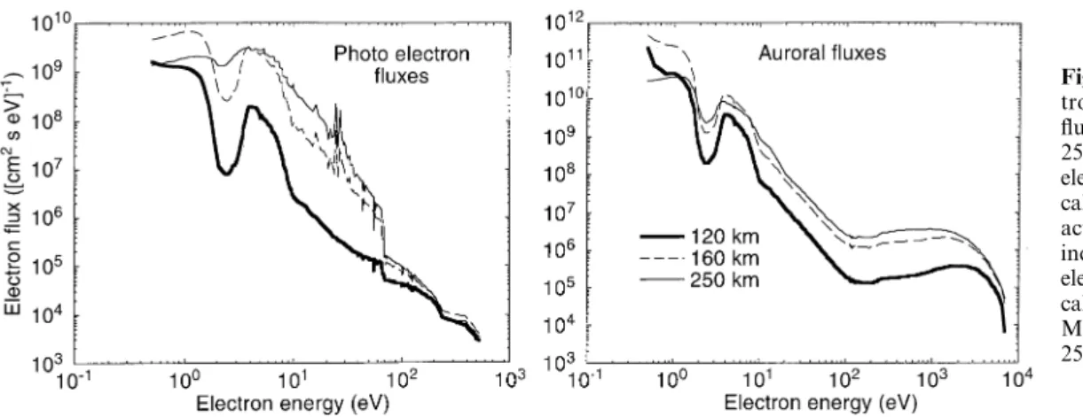
Fig. 1. Model photo elec-tron and auroral elecelec-tron fluxes for 120, 160 and 250 km altitudes. The photo-electron fluxes have been calculated for high solar activity conditions, f10.7 index"180. The auroral electron fluxes have been calculated using a 1 keV Maxwellian primary flux of 25 ergs/cm2/s

waves, but involve only particles of average energy, and will thus tend to push the wave intensity towards its thermal level.

2.2 Plasma line temperature

The different terms presented in Sect. 2.1 can be put together in a simple and elegant expression giving the intensity of the Langmuir waves (e.g. Yngvesson and Perkins, 1968). The intensity is usually measured in ‘plasma line temperature’,¹

p, defined as the temperature

of a Maxwellian plasma giving the same wave intensity. This is natural, because the wave intensity increases with electron temperature. For higher intensities it is even more convenient to multiply by Boltzmann’s constant, and express the temperature in eV. Thus, denoting the one-dimensional thermal (Maxwellian) and suprathermal electron distributions f

m(v) and fs(v) respectively, and the

collisional damping terms, we get:

K¹

p"

K¹

e(fm(v”)#fs(v”)#s) f

m(v”)!K¹e

d

dEfs(v”)#s

, (3)

whereKis Boltzmann’s constant,¹

ethe electron

temper-ature, v

”"upl/k is the phase velocity of the Langmuir

waves which scatter the radar signal, at frequencyu pland

scattering wave vectork, and the collision term is given by

s"neK¹eve mnkv4_” ,

v

e"ven#vei,

v

en"5.4]10~16nn(¹e)0.5,

v

ei"[34#4.18 log (¹3e/cne]10~6))]][(ne]10~6)/¹1.5e ],

(4)

where n

n is the neutral number density, ne the plasma

number density andm

ethe electron mass (Newman and

Oran, 1981, Nicolet, 1953). The collisional term dominates the damping below 110 km (Oranet al., 1981).

The effects of a magnetic field can be taken into ac-count by replacing the thermal Maxwellian distribution

with (Yngvesson and Perkins, 1968):

f(v

”)"ne

A

m

e

2nk¹

e

B

0.5 =

+

j/~=

exp (!bsin2h) cosh

]I_j(bsin2h)·exp

A

!(y!j)2

2bcos2h

B

. (5)

whereIjis the modified Bessel function of the first kind, b"_k2K¹

e/meuc, y"upl/uc, uc the electron cyclotron

frequency and h the angle between the Langmuir wave vector and the magnetic field. In the examples that follow the field-aligned case is discussed unless otherwise stated.

2.3 Suprathermal electronfluxes

Both solar EUV radiation and auroral precipitation give rise to suprathermal electrons in the ionospheric plasma. These electrons will show considerable structure in their distribution, because of both loss and production pro-cesses varying over different energy ranges (e.g. Rees, 1988). Such structures will influence the ratio between damping and excitation of Langmuir waves, and therefore cause different plasma line enhancements in different en-ergy ranges. It is therefore important to use an as accurate model as possible of the suprathermal electron distribu-tion. We have used model calculations according to the procedure described by Lummerzheim and Lilensten (1994). Three sample photo electron and three auroral second-ary energy-flux spectra are shown in Fig. 1. In the lower altitude samples (Fig. 1; 120, 160 km) the most prominent feature of the spectra is the dip in the 2—4 eV region. At higher altitudes the 2—4 eV dip, caused by excitation of vibrational levels in N

2, is less prominent. As was shown by Kirkwood et al. (1995), this dip results in a very flat one-dimensional distribution function in the same energy range, giving low Landau damping. It can also be seen that in the auroral case a power law description of the flux is adequate between 10 eV and 100 eV, which covers the reasonable upper limit of plasma line frequencies for the high latitude incoherent scatter radars. In the solar EUV case, there is pronounced structure arising from photo electron production in the 10—30 eV range, especially at higher altitudes. As with the N

(4)

plasma line strength. Without competing influences, it is the shape of the suprathermal distribution that determines the plasma line enhancement, not the flux intensity. For a Maxwellian distribution the plasma line temperature will always be the temperature of the Maxwellian for all resonant energies and flux intensities. When there are competing influences, i.e. in the region of low phase energy where the number of thermal electrons is comparable to the number of suprathermal electrons and in the region of high phase energy where the suprathermal fluxes fall to so low levels that their effect becomes comparable to the collision term, the flux intensity of the superthermal distri-bution will matter for the relative importance of the differ-ent terms. For example, the plasma line temperature for fluxes 100 times those shown in Fig. 1 give further en-hancements of less than 40% at 160 and 250 km altitude, if the resonant electrons are below 20 eV, as in these condi-tions, collisions have little effect. At 120 km collisional terms are important compared to the model fluxes used here, and an increase of the flux 100 times gives significant plasma line temperature enhancements (up to 4 times larger). At the boundary between the thermal and the superthermal region the level of suprathermal flux should also be important for the plasma line enhancement. The transition region between thermal and suprathermal influ-ence is usually at rather low energy (below about 2 eV) and rather narrow, and primarily affects plasma lines in the F region where the electron temperature is highest. Unless the measurements are made in one of those regions where either collisions or thermal damping are significant, it is not feasible to estimate suprathermal electron fluxes from plasma line measurements.

3 Measurement techniques

3.1 Radar technique

The primary technique of measuring incoherent scatter plasma line strength is that of using filter banks. A number of channels are used to measure the backscattered signal power, each covering a different, narrow, frequency band. These can cover a broad frequency range together. It is also possible to monitor several plasma line frequencies at once with each filter, by transmitting several different frequencies. From each altitude range there will be only one plasma line frequency, and it is thus possible to judge a posteriori which transmitted signal caused the return signal (e.g. Fredriksenet al. 1989).

It is also possible to measure frequency spectra, in either narrow or wide filters. This is most useful at the peak of the F region, where the electron density maximum gives a clear plasma line frequency maximum, and thus a clear frequency cut-off of the signal. By chirping the radar (Birkmayer and Hagfors, 1986) it is possible to create an artificial maximum in the returned signal by matching the plasma line frequency gradient with a trans-mitter frequency gradient. For bi- or tristatic systems the limited scattering region for the remote sites will give an essentially Gaussian shape of the measured spectra, allow-ing for spectral measurements from any altitude.

3.2 Analysis technique

The plasma line temperature is calculated from the ob-served power in the incoherent scatter measurements, using the expression of Yngvesson and Perkins (1968), Eqs. 16 and 17 transformed to SI units:

K¹

p"

A

plCsPrpr2p

P

tdrp

, (6)

where C

s is the system constant (Kirkwoodet al. 1986),

P

rpis the power received in the plasma line channel,rpis

the range to the scattering volume,dr

pis the range

contri-buting to the scattered plasma line signal and P

t is the

transmitted signal. This is essentially the same as the equation relating incoherent scatter ion line strength to the raw electron density. The factorA

plreflects both the

different scattering cross section of Langmuir waves as compared to ion acoustic waves, and the possible different radar gains over the frequency interval covered by the returned plasma line signal. Thus,

A

pl"gBe2/e0k2, (7)

where gis a gain factor found by calibration (using e.g. observations of radio stars),ethe electron charge,e

0the permittivity of free space andkthe wave number of the scattering wave.

The most difficult factor to estimate is the range contri-buting to the scattered plasma line signal, dr

p. The

re-ceived signal is the convolution of the transmitted pulse and the altitude profile of the scattered power. In the E region, the scattering region is typically smaller than the range resolution of the measurements, and the best es-timation is achieved by using measured plasma frequen-cies (from all available filters in a filter bank) to define the plasma line frequency-altitude profile. The range contri-buting to each receiver filter band can then be calculated. This has been described in detail by Kirkwood et al. (1995).

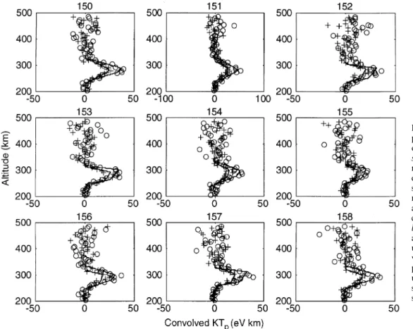
In F-region experiments, both scattering volume and pulse length are typically larger than the range gating. The plasma line power profiles thus show how the returned power increases with time (normally interpreted as range) as more and more of the pulse and the scattering region overlap. If the pulse length is longer than the scattering range, then the maximum backscattered signal will be obtained when all of the scattering region is illuminated by the pulse. Otherwise maximum signal will be for the time all of the signal illuminates part of the scattering region. In Fig. 2 a number of such plasma line power profiles are shown. One can note that the signal is not constant at the peak, but slightly increases with height. This is because the decrease of the received signal with r

p cannot be ignored. drp is not negligible

compared to r

p, and if the nominalrp for the gates are

used to getK¹

paccording to formula (7) (convolved with

(5)

Fig. 2. Altitude profiles of plasma line intensity at 6.4 Mhz on 6 August 1990. The ‘#’

signsdenote the upshifted sig-nal, and the ‘s_{’ denote the} downshifted signal. The mea-sured signal is multiplied with nominal gate range squared, and not compensated for differ-ent receiver gains. Thesolid linesare least square fits of a theoretical function [a single, uniform scattering range con-volved with a 54 km (360ls) pulse, and compensated for the use of nominal gate range to the scattering region in the mea-sured data]

throughout, and are fitted to the data using least squares.

For frequency spectra measurements at the peak of the F region, only one signal gate will be obtained. The shape of the spectra is determined by the enhancement and scattering range interval for the observed frequencies. To compare measurements with the predictions, the simplest approach is to use ion line measurements to calculate the plasma line frequency as a function of altitude, and through that calculate the scattering range interval.

It is important to note that it is the plasma line temper-ature times the length of the illuminated region that gives the basic signal strength. We will use ’convolvedK¹p@in this study to denote this. To calculate the actual signal strength received by the radar, one must take system noise, system constant and transmitted power into account using the following formula for signal to noise ratio,SNR:

SNR" PtdrpK¹p r2

pAplCsK¹BackDf

, (8)

where¹

Backis the background temperature, i.e. the system

noise, andDfis the receiver bandwidth.

4 Predictions and tests

4.1 Predictions

The predictions are presented in subsequent sections, or-dered after radar system. Two cases are presented, quiet

daytime conditions and auroral conditions. Though there are differences in neutral atmospheric density and photo electron fluxes between high and low solar activity, the main difference concerning plasma line measurements is in the electron density. Thus the predictions (made using high solar activity values) will be useful for both high and low solar activity. The differing electron densities (and thus plasma frequencies) generally present at solar max-imum and solar minmax-imum will however greatly affect the potential to measure plasma lines.

Predictions for three altitudes will be plotted, 120, 160 and 250 km. The height of 120 km is one where collisions are still important (for the neutral atmosphere and photo electron fluxes used), 160 km is high enough for collisions to be basically negligible, and 250 km is a typical altitude for the peak of the F region. The electron temperature will be important for the lowest plasma line frequency observ-able, and is set to typical values of 400, 1000 and 2000 K for the respective altitudes. Neutral densities used were taken from the MSIS-90E model (Hedin, 1987, 1991), using f10.7 index 180 and Ap index 19, day of year 183. For daytime measurements (local time 12) the neutral densities were 4.1 1017, 3.2 1016and 2.9 1015m~3, and the neutral temperatures 413, 926 and 1250 K for 120, 160 and 250 km altitude respectively. For the auroral night-time conditions (local time 24) the corresponding values used were 4.5 1017, 3.5 1016 and 2.7 1015m~3, 394, 801 and 1020 K.

(6)

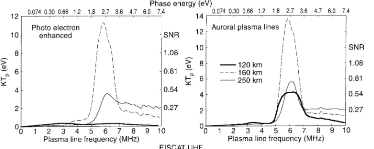
Fig. 3. Predicted plasma line strength for the EISCAT UHF radar for daytime and auroral conditions and three different altitudes. The

left y-axisgives the plasma line temperature in eV, theright y-axis

the F-region (250 km) signal-to-noise ratio for typical conditions (see

text for details). Thelower x-axisgives the plasma line frequency, while theuppergives the phase energy for the resonant electrons (for comparisons with Fig. 1)

typical for auroral precipitation although higher energies of a few keV are not unusual. As the resonant electrons driving Cherenkov emission for all realistic plasma line cases are well below the energies of typical primary fluxes, the predictions should be representative for most auroral cases. Higher energy primary fluxes will, however, deposit most of their energy at lower altitudes, which causes stronger secondary fluxes and therefore stronger plasma line enhancements at lower altitude than our sample flux. Examples of such fluxes giving much stronger enhance-ment at 120 km than in our prediction have been de-scribed by Kirkwoodet al. (1995).

The signal-noise ratio (SNR) will also be given to-gether with the plasma line temperature. As this predic-tion is most important for the measurement of frequency spectra at the peak of the F region, the conversion factor fromK¹

pto SNR has been calculated for an altitude of

250 km, a scattering range interval of 30 km (which re-quires a pulse length larger than 200ls) and a receiver bandwidth of 100 kHz (experimental values from Nilsson et al., 1996). It has also been assumed that the cut off is centered in the received frequency interval, as will typically be the case for actual measurements. This is im-portant only for comparisons between estimated ex-perimental SNR and the prediction. Radar system con-stant, system noise and transmitted power vary for the different radars, and the values used are given in the appropriate sections below. To use the SNR for the other altitudes, it is possible to compensate for the range differ-ence (according to Eq. 8), and divide by 30 to get the SNR per scattering km. The actual values of the scattering range will vary much more in the dynamic E region (during aurora) than in the F region.

4.2 Tests

The theoretical results have been tested by comparison with EISCAT UHF and VHF measurements. Power pro-files that can be analyzed using Eq. 6 have been used to

calculate the plasma line temperature from the measure-ments. For measurements at the peak of the F region the expected signal strength has been calculated using the ion line results (according to Eq. 8), and compared to the measured signal strength (SNR) over the receiver band-width. The measured SNR is the ratio of the range gate containing the F-region peak (cut-off) plasma line signal to an empty gate (lowest received power). This compari-son is made also for the remote sites. For the remote sites, the receiver bandwidth was 1 MHz, and the SNR over the total bandwidth was negligible. Instead an interval of 20 kHz around the peak was used.

4.3 The EISCAT UHF and Søndre Strømfjord radars

With scattering wave numbers of about 39 and 56 m~1, these two radar systems represent the upper range in scattering wave number. As the energy range of interest for plasma line enhancements is that corresponding to the phase velocity of the scattering wave (u

pl/k), this means

the lowest energy range for the suprathermal electrons. This of course also means that for low-enough plasma line frequencies or high-enough electron temperatures the res-onant particles may fall within the thermal region, and no plasma line enhancement is obtained. The predictions for the EISCAT UHF are shown in Fig. 3 and for Søndre Strømfjord in Fig. 4. The system constant used for EIS-CAT UHF was C

s"1.8 1027(defined for Eq. 8, actually

C@

s·c0/2 where c0is the speed of light and C@s the more

(7)

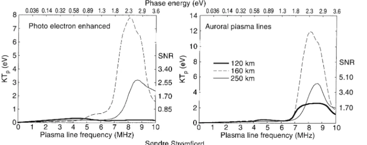
Fig. 4. Predicted plasma line strength for the Søndre Strømfjord radar for daytime and auroral conditions and three different alti-tudes. Theleft y-axisgives the plasma line temperature in eV, the

right y-axisthe F-region (250 km) signal-to-noise ratio for typical

conditions (see text for details). Thelower x-axisgives the plasma line frequency, while theuppergives the phase energy for the reso-nant electrons (for comparisons with Fig. 1)

the system constant used was C

s"3.3 1027 (from

Valladareset al., 1988), system noise 110 K and the trans-mitted power 4 MW. The large wave number and high transmitted power give a very good SNR for the Søndre Strømfjord radar. But if up and downshifted plasma lines cannot be measured simultaneously, which has been the case with the Søndre Strømfjord radar, the statistics are correspondingly reduced. Further, the pulse repetition used for the EISCAT UHF above is on the limit of the capabilities of the Søndre Strømfjord radar (with a duty cycle of 3%), so significantly higher SNR may be needed with the Søndre Strømfjord radar to achieve good fre-quency spectra estimates. In practice, plasma frequencies above 7 MHz seem to be needed for F-region plasma line measurements at Søndre Strømfjord (C. Heinselman, pri-vate communication), in agreement with our prediction of a sharp increase inK¹

pat such frequencies.

The predictions for the auroral E region have been discussed in detail by Kirkwoodet al. (1995), and have been found to agree very well with both the measurements of the authors (from the EISCAT UHF radar) and those of Valladares et al. (1988) from the Søndre Strømfjord radar. Note that Valladares et al. (1988) present their signal strength in K relative to the system noise of 110 K, which is almost the same as SNR. The maximum signal strength detected was 40 K, which corresponds to anSNR of 36%. Estimating the altitude to 140 km, setting the wave intensity to 7 eV (Valladareset al.’s estimation) and the scattering range to 500 m, our model predicts anSNR of 32%.

Daytime E-region measurements have been published (Bjørnas and Kirkwood, 1986) for low plasma line frequen-cies of 3—4.25 MHz. These are from a range between the thermal region (no enhancement) and the photoelectron enhanced region. Simulations like those shown in Fig. 3, but using altitudes and electron temperatures given in the paper of Bjørnas and Kirkwood (1986), give plasma line temperatures in the range 0.2—0.6 eV, well consistent with those observed except for two measurement points of 1 eV plasma line temperature at 3.25 and 3.5 MHz and

Fig. 5. Comparison between measured and predicted

signal-to-noise ratio for plasma line measurements at the peak of the F region on 27 July 1993. Thethick gray linedenotes mesuredSNR, thethin black lineis the theoretical value calculated from ion line parameters

130—140 km. This is about a factor of 2 more than ex-pected which might possibly be explained by an under-estimated scattering range interval in the calculation of the measured plasma line temperature.

(8)

Fig. 6. Predicted plasma line strength for the EISCAT UHF remote sites (Kiruna and Sodankyla¨) for daytime and 250 km altitude. The

the signal-to-noise ratio for a typical experimental configuration (see

sites is shown in Fig. 6. The electron temperature has been assumed to be 2000 K, the transmitted signal to be field aligned from Tromsø, and the altitude to be 250 km. The wave numbers of the scattering waves for Kiruna were k"36.1 m~1and for Sodankyla¨k"33.3 m~1. The main reasons for the stronger signal in Kiruna are geometrical; for Sodankyla¨ the scattering volume is smaller (giving a factor of 2 difference as compared to Kiruna), and the range to the scattering volume is larger (giving about 50% further difference). The lowerkvector for Sodankyla¨ gives a further reduction of about 15%, and finally the larger wave vector angle to the magnetic field pushes the en-hancement of the plasma line to slightly higher frequen-cies.

The average SNR value observed in Kiruna was 16% during the period when clear signals were received, in good agreement with the prediction of 18% for the same time interval. Some weak plasma lines were also obtained at Sodankyla¨, with SNR reaching at most 5%, also in accordance with the theory.

For the auroral F-region case, plasma line power pro-files are available from filter bank experiments on 6 Au-gust 1990. These have been analyzed by fitting theoretical functions to the measured profiles, as discussed earlier and shown in Fig. 2. The fit consists of a minimization of the square of the difference between the model and the data. This minimization is time consuming, and sometimes fails. Thus, the fit must be manually inspected as can be done in Fig. 2. The advantage with this fit is that both the upper and lower slope and the (relatively) constant peak depend on the scattering range (and the pulse length which is known). The plasma line temperature from this analysis for the plasma line frequency of 6.4 MHz is relatively constant at around 0.7 eV for the event shown in Fig. 2. Simulations of the same time period give results averaging around 0.6 eV. This may seem low compared to the prediction in Fig. 3, the reasons being a higher electron temperature (often more than 2500 K), and an angle of 13° to the geomagnetic field during the experiment in question.

4.4 The EISCAT VHF radar

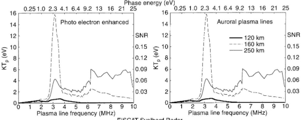
With a frequency of 224 MHz and wave number of about 9.6 m~1, the electron energy range of interest to the EISCAT VHF radar is considerably higher than for the previously described radars. For most auroral cases the resonant electrons will be in the power law region above 10 eV described in Sect. 2.4 and shown in Fig. 1 (right-hand panel), giving enhancements as shown in Fig. 7. In the photo electron case the structure in the 10—20 eV region will prove to be of great importance, as can also be seen in Fig. 7 (left-hand panel). For the SNR scale, a sys-tem constant of 4.5 1026, a syssys-tem sys-temperature of 200 K and a transmitted power of 1.5 MW were used. Note also that an angle of 13 degrees to the geomagnetic field has been used.

During the plasma line campaign in July 1993 de-scribed in Nilsson et al. (1996) the VHF radar was run simultaneously. Only a few very weak plasma lines were detected, at the end of the campaign when the plasma line frequency fell below 6 MHz. This is consistent with the low predicted SNR as shown in Fig. 7, increasing slightly towards lower frequencies.

A better test can be made by simulating the very good measurements published by Fredriksenet al. (1989). The signal strength is represented with the parameter ‘Q’ in their paper, which is essentially the convolvedK¹

pused in

(9)

Fig. 7. Predicted plasma line strength for the EISCAT VHF radar for daytime and auroral conditions and three different altitudes. The

the F-region (250 km) signal-to-noise ratio for typical conditions (see

Table 1. The first row shows the approximate altitude of a plasma

line scattering region, as estimated from plate 1 of Fredriksenet al. (1989). Row two shows frequency of the observed plasma lines, going from 4 up to 5 MHz, and then back down to 4 MHz above the peak

of the F region. Row 3 shows the plasma line signal strength as logQ, whereQis defined in the paper of Fredriksenet al. (1989), whereas row 4 shows the logQvalues obtained from a simulation using the model fluxes presented in this study

Altitude (km) 150 165 185 190 200 222 245 255 265 280 290

Frequency (MHz) 4.0 4.2 4.4 4.6 4.8 5.0 4.8 4.6 4.4 4.2 4.0

LogQmeasured 8.7 9.4 8.9 8.9 9.3 9.9 9.7 9.7 9.2 9.4 9.7

LogQsimulated 8.6 9.4 8.8 8.6 9 9.8 9 8.8 9.4 9.5 9.6

computed and convolved with the transmitted pulse to achieve the maximum returned signal from the different scattering regions. This simulation can then be compared to the measured plasma line signal. The comparison for a sample time (10:10 UT) is given in Table 1. In the com-parison it is important to note that in these measurements two different pulse lengths were used, 110 and 210ls, not two 210ls as is said in the paper (Fredriksen, private communication). Most features of the observations can be correctly modelled, as summarized in Table 1, i.e. the strong collisional damping of the lower 4-MHz plasma line, and the strong high altitude 4.0-, 4.2-, 4.4-MHz plasma lines. The observations from the high-altitude 4.6-and 4.8-MHz plasma lines appear strong compared to the prediction, but this may have to do with scattering range estimations. The same can account for the lower 4.2 MHz being stronger than the 4.4 MHz, which is correctly modelled through a larger scattering range. In the Fred-riksenet al. (1989) data there is also a clear time variation in the lower 4.2-MHz plasma line strength. This is well correlated with a varying altitude of the scattering region, with the higher altitudes giving stronger plasma line sig-nals. This can be explained by lower collisional damping at the higher altitude and agrees well with simulations. The data set clearly show that there are strong enhance-ments in the 4—5 MHz region, in accordance with the prediction.

4.5 The EISCAT Svalbard radar

The EISCAT Svalbard radar will operate with a frequency of 500 MHz, and the scattering wave number will thus be about 21 m~1. Predictions for daytime and auroral condi-tions are shown in Fig. 8. The system constant used for calculating SNR was the same as for EISCAT UHF, C

s"1.8 1027, the system temperature was set to 150 K,

and the transmitted power 0.5 MW. The SNR values obtained are quite low, partly because of the low transmit-ted power but also because of the k vector dependence giving a factor about 4 less than for example, the EISCAT UHF radar. As can be seen the EISCAT Svalbard radar can be expected to see enhanced plasma lines over a broad frequency range, but the SNR may be too low to allow for good plasma line spectra measurements at the peak of the F region, unless the transmitter power can be increased.

5 Summary

(10)

Fig. 8. Predicted plasma line strength for the EISCAT Svalbard radar for daytime and auroral conditions and three different alti-tudes. Theleft y-axisgives the plasma line temperature in eV, the

right y-axisthe F-region (250 km) signal-to-noise ratio for typical

conditions (see text for details). Thelower x-axisgives the plasma line frequency, while theuppergives the phase energy for the reso-nant electrons (for comparisons with Fig. 1)

best electron drift resolution (due to the proportionality of the Doppler shift to the wave number), as compared to the lower frequency radars (i.e. EISCAT VHF and Svalbard). The lower frequency radars on the other hand, show en-hancement of the plasma lines over a much broader fre-quency range, and can be used also during low solar activity. In the auroral E region, where the electron density (plasma line frequency) depends on the incident energetic precipitation, the EISCAT UHF and Søndre Strømfjord radars are once more the preferred choice. The strong enhancement in the N

2dip region give strongly enhanced plasma lines for typical auroral conditions (5—7-MHz plasma line frequency for the EISCAT UHF).

Concerning the use of plasma lines to determine supra-thermal fluxes, it is found that for typical EISCAT UHF/Søndre Strømfjord F-region measurements, the phase energies of the resonant electrons are in an interval where a determination of the intensity of the flux is depen-dent on the competing influence of the thermal electrons. At the peak of the F region the thermal plasma is usually hot enough that there is some competition in influence between the thermal and suprathermal distributions for typical plasma line frequencies of 5—7 MHz (depending on electron temperature). Comparison between the strength of the up- and downshifted plasma line enhancement can then be used to estimate the relative upward and down-ward flux of electrons. However, such differences will most likely be small. The gain over the received frequency range may vary about as much (some 10%) and must be careful-ly estimated (for example using radio stars). Frequency differences between the up- and downshifted plasma lines may also be a problem for estimating flux anisotropy, especially at the peak of the F region where the cut-off may occur within the receiving bandwidth. Such anisot-ropies close to the thermal region and at the resonance frequency of the plasma line may however influence the dispersion of the plasma line (e.g. Nilssonet al., 1996). It is thus worthwhile to use plasma lines to try to study such anisotropies experimentally.

For the resonant energies appropriate for typical EIS-CAT VHF measurements, the collisional influence is

typi-cally significant and thus allows for determination of suprathermal fluxes using plasma lines. However, using 100 times our model flux still gives further plasma line enhancements of less than 4 times, so the accuracy of the method is limited.

Acknowledgements. Topical Editor D. Alcayde´ thanks T. van Eyken and another referee for their help in evaluating this paper.

References

Birkmayer, W., and T. Hagfors,Observational technique and

para-meter estimation in plasma line spectrum observations of the ionosphere by chirped incoherent scatter radar,J.Atmos.¹err.

Phys.,48,1009—1019, 1986.

Bjørnas, N., and S. Kirkwood,Observations of natural plasma lines in

the E region and lower F region with the EISCAT UHF radar,

Ann.Geophysicae,4,137—144, 1986.

Bjørnas, N., and S. Kirkwood,Derivation of ion composition from

a combined ion line/plasma line incoherent scatter experiment, J.

Geophys.Res.,93,5787—5793, 1988.

Fredriksen, A_s, N. Bjørnas, and T. L. Hansen, The first EISCAT

two-radar plasma-line experiment, J. Geophys. Res., 94,

2727—2731, 1989.

Hagfors, T., and M. Lehtinen,Electron temperature derived from

incoherent scatter radar observations of the plasma line fre-quency,J.Geophys.Res.,86,119—124, 1981.

Hedin, A. E.,MSIS-86 thermospheric model,J.Geophys.Res.,92,

4649, 1987.

Hedin, A. E.,Extension of the MSIS thermosphere model into the

middle and lower atmosphere,J.Geophys.Res.,96,1159—1172, 1991.

Heinselman, C. J., and J. F. Vickrey,On the frequency of Langmuir

waves in the ionosphere,J.Geophys.Res.,97,14905—14910, 1992.

Ichimaru, S.,Statistical Plasma Physics volume1:Basic Principles,

Addison Wesley, 1992.

Kofman, W., J.-P. St.-Maurice, and A. P. van Eyken,Heat flow effect

on the plasma line frequency,J.Geophys.Res.,98,6079—6085, 1993.

Kirkwood, S., and N. Bjørnas,Electron temperatures determined by

tristatic plasma line observations with the EISCAT UHF inco-herent scatter radar,Geophys.Res.¸_ett_.,_19,₆₆₁_—_{664, 1992.}

Kirkwood, S., P. N. Collis, and W. Schmidt,Calibration of electron

densities for the EISCAT UHF radar, J. Atmos. Terr. Phys.48,

(11)

enhanced incoherent-scatter plasma lines in aurora,J.Geophys.

Res.,100,21343—21355, 1995.

Lummerzheim, D., and J. Lilensten,Electron transport and energy

degradation in the ionosphere: evaluation of the numerical solu-tion, comparison with laboratory experiments, auroral observa-tions,Ann.Geophysicae,12,1039—1051, 1994.

Newman, A., E. Oran,The effects of electron-neutral collisions on the

intensity of plasma lines,J.Geophys.Res.,86,4790—4794, 1981.

Nicolet, M.,The collision frequency of electrons in the ionosphere,J.

Atmos.¹_err_._Phys_.,_3,₂₀₀_—_{220, 1953.}

Nilsson, H., S. Kirkwood, and N. Bjørnas,Bistatic measurements of

incoherent-scatter plasma lines, J. Atmos. ¹err. Phys., 58,

175—188, 1996.

plasma lines: a first comparison of theory and experiment, J.

Geophys.Res.,86,199—205, 1981.

Perkins, F., and E. E. Salpeter, Enhancement of plasma density

fluctuations by nonthermal electrons,Phys.Rev.,139,A55—62, 1965.

Rees, M. H.,Physics and Chemistry of theºpper Atmosphere,