Analysis of Stochastic Gilpin-Ayala Model in
Polluted Environments
Zongjie Geng, Meng Liu
∗Abstract—In this paper, we consider a stochastic Gilpin-Ayala model in polluted environments. Firstly, sufficient conditions for extinction, non-persistence in the mean, weak persistence and stochastic permanence of the species are established. The threshold between extinction and weak persistence is obtained. Then global attractivity of the model is studied. Finally, several numerical figures are introduced to validate the results.
Index Terms—environmental pollution, stochastic noises, per-manence, extinction.
I. INTRODUCTION
W
ITH the rapid development of industries and agricul-ture, many toxins are emitted into the environment. These toxins have let lots of species go to extinction and let many be on the verge of extinction. This motivates scholars to investigate the effects of toxins on populations and to establish theoretical persistence-extinction thresholds of the species.In recent years, many authors have investigated the effects of toxins on species by using mathematical models. Hallam and his colleagues did pioneering work in [1], [2], [3], where the authors proposed some deterministic population models with toxin effect and established the theoretical persistence-extinction thresholds for their models. From then on, many interesting and important population models with toxin effect were proposed and analyzed. The authors in [4], [5], [6], [7], [8], [9], [10], [11] considered single-species population models in a polluted environment; The authors in [12], [13], [14] investigated the effected of toxins on the persistence and extinction of multi-species models; The studies [15], [16] analyzed the population models with impulsive toxi-cant input; Stage-structured population models in a polluted environment were studied by [17], [18].
However, the growth of species in the natural world is inevitably affected by environmental noises (May [19]). Therefore several authors considered stochastic population models in a polluted environment, see e.g. [20]-[26]. Espe-cially, Liu and Wang [21] have investigated the following
Manuscript received January 17, 2015; revised February 20, 2015. This work was supported by the National Natural Science Foundation of China (Nos. 11301207, 11171081, 11301112 and 11171056), Natural Science Foundation of Jiangsu Province (No. BK20130411), Natural Sci-ence Research Project of Ordinary Universities in Jiangsu Province (No. 13KJB110002), Qing Lan Project of Jiangsu Province (2014).
M. Liu is with the School of Mathematical Science, Huaiyin Normal University, Huaian 223300, PR China e-mail: [email protected].
Z. Geng is with Huaiyin Normal University.
stochastic single-species model with toxin effect:
dx(t) =x(t)[r0−r1C0(t)−ax(t)]dt+σ1x(t)dB1(t)
dC0(t) = [kCe(t)−(g+m)C0(t)]dt
dCe(t) = [−hCe(t) +u(t)]dt
(1) wherex(t)is the size of the population; r0 >0 stands for the intrinsic growth rate of the population without toxicant; r1 > 0 denotes the population response to the pollutant present in the organism;C0(t)andCe(t)represent the con-centration of toxicant in the organism and in the environment, respectively;B1(t)is a standard Brownian motion defined on a complete probability space(Ω,F,P);σ2
1is the intensity of the white noise;k >0stands for the organism’s net uptake rate of toxicant from the environment; g > 0 and m > 0
represent the egestion and depuration rates of the toxicant in the organism, respectively;h >0 denotes the toxicant loss rate from the environment by volatilization and so on;u(t)
is a non-negative bounded continuous function defined on
[0,+∞)representing the exogenous rate of input of toxicant into the environment. Liu and Wang [21] have obtained the persistence-extinction threshold and established the sufficient conditions for stochastic permanence of the species.
Based on the study [21], some interesting and important questions arise naturally:
(Q1) Model (1) is based on the classical Logistic equation. Gilpin and Ayala [27] have pointed out that Logistic equation has some limitations to describe the reality in some cases and have proposed Gilpin-Ayala model. Then what happens if the model in [21] is replaced by Gilpin-Ayala model?
(Q2) Model (1) assumes that only the growth rate r0 is affected by random noise. Then what happens if all parameters are affected by random noise? In fact, May [19] have pointed out that due to environmental noise, the growth rate, competition rate and other parameters in population models should be stochastic.
(Q3) The conditions of stochastic permanence in [21] are too restricted, can we improve them?
(Q4) In the study of population models, global attractivity of the solution is one of the most important topics. Then, is the solution of the underlying model globally attractive?
stochastic single-species model with toxicant effect:
dx(t) =x(t)[r0−r1C0(t)−axθ(t)]dt+σ1x(t)dB1(t)
+σ2C0(t)x(t)dB2(t) +σ3x1+θ(t)dB3(t),
dC0(t) = [kCe(t)−(g+m)C0(t)]dt,
dCe(t) = [−hCe(t) +u(t)]dt,
(2) whereθ >0is a constant,B1(t),B2(t)andB3(t)are inde-pendent standard Brownian motions defined on(Ω,F,P). It is easy to see that if θ = 1and σ2 =σ3 = 0, then model (2) becomes model (1).
In Section 2, we carry out the survival analysis for model (2). Sufficient conditions for extinction, non-persistence in the mean, weak persistence and stochastic permanence of the species are established. The threshold between extinction and weak persistence is obtained. The results in [21] are improved and extended. In Section 3, we show that model (2) is globally attractive. In Section 4, we extend these results to a n−species model. In Section 5, some numerical simulations are given to illustrate the main results. In the last section, we give conclusions.
II. PERSISTENCE AND EXTINCTION
BothC0(t)andCe(t)in model (2) are concentrations, so we should give some conditions under which 0 ≤C0(t)<
1, 0≤Ce(t)<1. In fact, we have
Lemma 1. ([21]) If0< k≤g+m, lim sup
t→+∞ u(t)≤h,
then
0≤C0(t)<1, 0≤Ce(t)<1for all t≥0.
From now on, we always suppose that 0 < k ≤ g+ m, lim sup
t→+∞
u(t) ≤ h. Note that the last two equations in model (2) are linear with respect to C0(t) andCe(t), it is easy to obtain their explicit solutions. So in the following study, we need only to consider the first equation in model (2), that is
dx(t) =x(t)[r0−r1C0(t)−axθ(t)]dt+σ1x(t)dB1(t)
+σ2C0(t)x(t)dB2(t) +σ3x1+θ(t)dB3(t).
(3) Note that x(t) in Eq.(3) represents the population size, then x(t) should be nonnegative. So first of all, we must show that for any given positive initial value, Eq. (3) has a unique global positive solution.
Lemma 2. For any initial datax(0) =x0>0, Eq. (3) has a unique global positive solutionx(t)almost surely (a.s.).
Proof: The proof is similar to that of Theorem 4.1 in
[28] and hence is omitted.
Before we state and prove our main results, we recall some important definitions.
Definition 1. (i) x(t) is said to go to extinction if
lim
t→+∞x(t) = 0.
(ii) x(t)is said to be non-persistent in the mean if there is a positive constant β such that
lim t→+∞t
−1∫ t 0
xβ(s)ds= 0.
(iii) x(t) is said to be weakly persistent ([4]) if
lim sup t→+∞
x(t)>0.
(iv) x(t) is said to be stochastically permanent ([29]), if
for every 0 < ε < 1, there are positive constants β
and M such that lim inf
t→+∞P{x(t) ≥ β} ≥ 1 − ε and lim inf
t→+∞P{x(t)≤M} ≥1−ε.
Theorem 1. Iflim sup t→+∞
t−1∫t
0b(s)ds <0, thenx(t)goes to extinction a.s., where
b(t) =r0−0.5σ21−r1C0(t)−0.5σ22C02(t). Proof:By Itˆo’s formula
ln[x(t)/x0] = ∫ t
0 [
b(s)−axθ(s)−0.5σ2
3(s)x2θ(s) ]
ds
+σ1B1(t) +M2(t) +M3(t),
(4) where
M2(t) = ∫ t
0
σ2C0(s)dB2(s), M3(t) = ∫ t
0
σ3xθ(s)dB3(s). The quadratic variation ofM2(t)is
⟨M2(t), M2(t)⟩= ∫ t
0
σ22C02(s)ds≤σ22t.
It then follows from the strong law of large numbers for martingales(see e.g., [30], P.16) that
lim
t→+∞M2(t)/t= 0, a.s. (5)
The quadratic variation ofM3(t)is ⟨M3, M3⟩=
∫ t 0
σ32x2θ(s)ds. In view of the exponential martingale inequality,
P {
sup
0≤t≤k
[
M3(t)−
1
2⟨M3, M3⟩
]
>2 lnk
}
≤1/k2.
An application of the Borel-Cantelli lemma (see e.g. [30], P.10), for almost all ω ∈ Ω, there is a stochastic integer k0=k0(ω)such that fork≥k0,
sup
0≤t≤k
[
M3(t)−1
2⟨M3, M3⟩
]
≤2 lnk.
In other words, M3(t)≤2 lnk+ 0.5∫0tσ32x2θ(s)ds for all
0≤t≤k, k≥k0almost surely. Substituting this inequality into (4) gives
lnx(t)−lnx0 ≤
∫ t 0
(b(s)−axθ(s))ds+σ
1B1(t) +M2(t) + 2 lnk ≤
∫ t 0
b(s)ds+σ1B1(t) +M2(t) + 2 lnk
(6) for all 0 ≤ t ≤ k, k ≥ k0 almost surely. Hence for 0 <
k−1≤t≤k, k≥k0, we have
t−1
{lnx(t)−lnx0} ≤t−1∫0tb(s)ds
+σ1B1(t)/t+M2(t)/t+ 2(k−1)−1lnk.
Then by (19) and lim
t→+∞B1(t)/t = 0, we get lim sup
t→+∞
t−1lnx(t) ≤ lim sup
t→+∞
t−1∫t
0b(s)ds <0. Therefore
lim
Theorem 2. If lim sup t→+∞
t−1∫t
0b(s)ds= 0, thenx(t)is non-persistent in the mean a.s.
Proof: It is easy to see that for arbitrarily givenε >0, we can find a positive constantT1 such that
t−1
∫ t 0
b(s)ds <lim sup t→+∞ t
−1∫ t 0
b(s)ds+ε/2 =ε/4
for t > T1. Substituting this inequality into (6) gives
lnx(t)−lnx0
< εt/4−a
∫ t 0
xθ(s)ds+σ
1B1(t) +M2(t) + 2 lnk for allT1≤t≤k, k≥k0. Lett be sufficiently large such that T1≤T ≤k−1≤t≤k, k≥k0 and
σ1B1(t)/t≤ε/4, (lnk)/t≤ε/8, M2(t)/t≤ε/4. Consequently forT ≤k−1≤t≤k and k≥k0,
lnx(t)−lnx0≤εt−a ∫ t
0
xθ(s)ds.
Denote λ(t) =∫t
0xθ(s)ds. Therefore,
θ−1ln(dλ/dt)< εt
−aλ(t) + ln x0. Hence, eθaλ(t)(dλ/dt) < xθ
0eθεt. In other words, we have shown that
eθaλ(t)< eθaλ(T)+xθ0aε−1eθεt−xθ0aε−1eθεT. Taking the logarithm yields
λ(t)<(θa)−1ln{xθ
0aε−1eθεt+eθaλ(T)−xθ0aε−1eθεT }
.
Therefore,
lim sup t→+∞
{
t−1 ∫ t
0
xθ(s)ds
}
≤lim sup t→+∞ θ
−1a−1
× {
t−1ln {
xθ
0aε−1eθεt+eθaλ(T)−xθ0aε−1eθεT }}
.
It then follows from the L’Hospital rule that
lim sup t→+∞
{
t−1∫ t 0
xθ(s)ds
} ≤ε/a.
By the arbitrariness of ε that lim sup t→+∞
t−1∫t 0x
θ(s)ds ≤ 0.
Note thatx(t)≥0, then lim t→+∞t
−1∫t
0xθ(s)ds= 0.
Theorem 3. If lim sup t→+∞
t−1∫t
0b(s)ds > 0, then x(t) is weakly persistent a.s.
Proof: : To begin with, let us prove
lim sup t→+∞
lnx(t)
lnt ≤1, a.s. (7)
In fact, by Itˆo’s formula,
d(etlnx) =et
[
lnx+b(t)−axθ−0.5σ2 3x2θ
]
dt
+etσ
1dB1(t) +etσ2C0(t)dB2(t) +etσ3xθdB3(t).
Consequently, etlnx(t)−lnx
0
=
∫ t 0
es
[
lnx(s) +b(s)−axθ(s)−0.5σ2 3x2θ(s)
]
ds
+N1(t) +N2(t) +N3(t),
(8) where
N1(t) = ∫ t
0
esσ1dB1(s), N2(t) = ∫ t
0
esσ2C0(s)dB2(s),
N3(t) = ∫ t
0
esσ
3xθ(s)dB3(s).
LetN(t) =N1(t)+N2(t)+N3(t).Note thatN(t)is a local martingale, whose quadratic variation is
⟨N, N⟩=
∫ t 0
e2s[σ2
1+σ22C02(s) +σ23x2θ(s)]ds. By the exponential martingale inequality,
P {
sup
0≤t≤µk
[
N(t)−0.5e−µk⟨N, N⟩
]
> ρeµklnk
} ≤k−ρ,
whereρ >1 andµ >0is arbitrary. By virtue of the Borel-Cantelli lemma, for almost allω∈Ω, there is ak0(ω)such that for everyk≥k0(ω),
N(t)≤0.5e−µk⟨N(t), N(t)⟩+ρeµklnk, 0≤t≤µk.
When this inequality is used in (8), one can see that etlnx(t)−lnx
0 ≤
∫ t 0
es
[
lnx(s) +b(s)−axθ(s)−0.5σ23x2θ(s) ]
ds
+0.5e−µk
∫ t 0
e2sσ2
1ds+ 0.5e−µk ∫ t
0
e2sσ2
2C02(s)ds
+0.5e−µk∫ t
0
e2sσ32x2θ(s)ds+ρeµklnk
=
∫ t 0
es
[
lnx(s) + 0.5es−µkσ2
1+ 0.5es
−µkσ2 2C02(s)
+b(s)−axθ−0.5σ2
3x2θ[1−es−µk] ]
ds+ρeµklnk.
Note that for arbitrary 0 ≤ t ≤ µk and x > 0, there is a constantC independent ofksuch that
lnx+b(t) + 0.5et−µkσ2
1+ 0.5et−µkσ22C02(t) −axθ−0.5σ2
3x2θ[1−et−µk]≤C. That is to say, for arbitrary0≤t≤µk, we have
etlnx(t)−lnx0≤C[et−1] +ρeµklnk. Thus ifµ(k−1)≤t≤µk andk≥k0(ω),then
lnx(t)/lnt ≤e−tlnx
0/lnt+C[1−e−t]/lnt
+ρe−µ(k−1)eµklnk/lnt.
Lettingk→+∞yieldslim sup t→+∞
lnx(t)
lnt ≤ρeµ.Lettingρ→1
andµ→0 gives the required assertion (21). Now suppose that lim sup
t→+∞
b(t) > 0, we prove
lim sup t→+∞
x(t) > 0 almost surely. If it is false, set F =
{lim sup t→+∞
x(t) = 0},and suppose thatP(F)>0. By (4),
t−1ln(x(t)/x
0) =t−1∫0tb(s)ds−t−1∫0taxθ(s)ds −0.5t−1∫ t
0
For arbitrary ω ∈ F, we have lim
t→+∞x(t, ω) = 0, it then
follows from the law of large numbers for local martingales that lim
t→+∞M3(t)/t = 0. When this identity and (5) are
used in (9), one can observe that lim sup t→+∞
[t−1lnx(t, ω)] =
lim sup t→+∞ t
−1∫t
0b(s)ds >0. Hence P{lim sup
t→+∞[t
−1lnx(t)]>
0}>0,which is a contradiction with (7).
Remark 1. From Theorems 1, 2 and 3, one can observe that lim sup
t→+∞ t −1∫t
0b(s)ds is the threshold between weak persistence and extinction of the species.
In the study of population system, permanence is one of the most important topics. So let us now consider the permanence ofx(t).
Theorem 4. If lim inf
t→+∞b(t)>0 and 0< θ≤1, thenx(t)is
stochastically permanent.
Proof: DefineV1(x) = 1/x1+θ,wherex >0. By Itˆo’s formula,
dV1(x(t)) = (1 +θ)V1(x) [
−r0+r1C0(t) +axθ ]
dt
+0.5(1 +θ)(2 +θ)σ2 1V1(x)dt
+0.5(1 +θ)(2 +θ)σ2
2C02(t)V1(x)dt
+0.5(1 +θ)(2 +θ)σ2 3xθ−1dt
−(1 +θ)σ1V1(x)dB1(t)−(1 +θ)σ2V1(x)C0(t)dB2(t) −(1 +θ)σ3x−1dB3(t).
Since lim inf
t→+∞b(t)>0, we can let0< κ <1 be sufficiently
small such that
lim inf
t→+∞b(t)>0.5κ(θ+ 1)(σ
2
1+σ22). (10) Define V2(x) = (1 +V1(x))κ. By Itˆo’s formula, for suffi-ciently larget,
dV2(x) =κ(1 +V1(x))κ−2× {
(1 +V1(x))(1 +θ) [
V1(x) (
−r0+r1C0(t) +axθ )
+0.5(2 +θ)σ2
1V1(x) + 0.5(2 +θ)σ22C02(t)V1(x)
+0.5(2 +θ)σ2 3xθ−1
]
+ 0.5(κ−1)(1 +θ)2 ×
{
σ2
1V12(x) +σ22C02(t)V12(x) +σ32x−2 }}
dt
−κ(1 +V1(x))κ−1(1 +θ) [
σ1V1(x)dB1(t)
+σ2C0(t)V1(x)dB2(t) +σ3x−1dB3(t) ]
≤κ(1 +θ)(1 +V1(x))κ−2× {
− [
lim inf
t→+∞b(t)−ε−0.5κ(θ+ 1)(σ
2 1+σ22)
]
V2 1(x) −
[
r0−r1−0.5(2 +θ)(σ21+σ22) ]
V1(x)
+a(V1(x) + 1)x−1+ (1 + 0.5θ)σ32(xθ−1+x−2) }
dt
−κ(1 +V1(x))κ−1(1 +θ) [
σ1V1(x)dB1(t)
+σ2C0(t)V1(x)dB2(t) +σ3x−1dB3(t) ]
,
whereεis sufficiently small satisfying
lim inf
t→+∞b(t)−0.5κ(θ+ 1)(σ
2
1+σ22)> ε.
In the proof of the last inequality, we have used the facts that C0(t)≤1 andκ < 1. Letη >0 be sufficiently small such that
0< η
κ(1 +θ)<lim inft→+∞b(t)−0.5κ(θ+ 1)(σ
2
1+σ22)−ε. DefineV3(x) =eηtV2(x). By Itˆo’s formula, for sufficiently larget,
dV3(x(t)) =ηeηtV2(x)dt+eηtdV2(x) ≤(1 +θ)κeηt(1 +V
1(x))κ−2
{η(1 +V 1(x))2
κ(1 +θ)
− [
lim inf
t→+∞b(t)−ε−0.5κ(θ+ 1)(σ
2 1+σ22)
]
V2 1(x) −
[
r0−r1−0.5(2 +θ)(σ21+σ22) ]
V1(x)
+a(V1(x) + 1)x−1+ (1 + 0.5θ)σ32(xθ−1+x−2) }
dt
−eηtκ(1 +V
1(x))κ−1(1 +θ) [
σ1V1(x)dB1(t)
+σ2C0(t)V1(x)dB2(t) +σ3x−1dB3(t) ]
=eηtJ(x)dt−eηtκ(1 +V
1(x))κ−1(1 +θ) [
(σ1dB1(t) +σ2C0(t)dB2(t))V1(x) +σ3x−1dB3(t) ]
where
J(x) = (1 +θ)κ(1 +V1(x))κ−2 {
− [
lim inf t→+∞b(t)
−ε−0.5κ(θ+ 1)(σ2
1+σ22)−
η κ(1 +θ)
]
V12(x) −
[
r0−r1−0.5(2 +θ)(σ21+σ22)−
2η κ(1 +θ)
]
V1(x)
+aV1(x)x−1+ η
κ(1 +θ)+ax −1
+(1 + 0.5θ)σ2
3(xθ−1+x−2) }
.
(11) Now we are in the position to prove if0< θ≤1, thenJ(x)
is upper bounded inR+. Let
K= min
{
1,
(
K1
4a
)−θ
,
(
K1
6σ2 3
)−2θ}
,
where
K1= lim inf
t→+∞b(t)−ε−0.5κ(θ+ 1)(σ
2
1+σ22)−η/[κ(1 +θ)]. (a) If x ≥ K, then by the definition of V1(x), J(x) is upper bounded, that is to say, there is a constant J1 > 0 such that sup
x≥K
J(x)< J1.
(b) Ifx < K, then by0< x <1and0< θ≤1, one can obtain that
xθ−1=x2θx−θ−1≤V
1(x). (12)
On the other hand, byx <
(
K1
4a
)−θ , we get
−0.25K1V12(x) +aV1(x)x−1<0. (13)
In the same way, byx <
(K
1
6σ2 3
)−2θ
one can show that
When (12),(13) and (14) are used in (11), we derive that
J(x)≤(1 +θ)κ(1 +V1(x))κ−2 {
−0.5K1V12(x)
+ η κ(1 +θ)−
[
r0−r1−0.5(2 +θ)(σ21+σ22) − 2η
κ(1 +θ)−(1 + 0.5θ)σ
2 3−a
]
V1(x) }
.
Hence if x < K, there is a positive constant J2 such that
supx<KJ(x) < J2. Therefore, J(x) is upper bounded in
R+, i.e., J3 := supx∈R+J(x) < +∞. Consequently, for
sufficiently larget,
dV3(x(t))≤J3eηtdt −eηtκ(1 +V
1(x))κ−1(1 +θ) [
σ1V1(x)dB1(t)
+σ2C0(t)V1(x)dB2(t) +σ3x−1dB3(t) ]
.
That is to say
E
[
eηt
(
1 +V1(x) )κ]
≤ (
1 +V1(x0) )κ
+J3 (
eηt−1
)
/η.
Hence
lim sup t→+∞ E
[
Vκ
1(x(t)) ]
≤J3/η. (15)
Therefore
lim sup t→+∞ E
[
x−κ−κθ(t)
]
≤J3/η=:J4.
For arbitrary ε > 0, let β = (ε/J4)−κ−κθ. It then follows from Chebyshev’s inequality that
P {
x−κ−κθ(t)> β−κ−κθ
} ≤E[x
−κ−κθ(t)] β−κ−κθ .
In other words, lim sup
t→+∞ P{x(t) < β} ≤ β κ+κθJ
4 = ε.
Therefore,lim inf
t→+∞P{x(t)≥β} ≥1−ε.
To complete the proof, it suffices to show that for arbitrary given ε > 0, there exists a constant M > 0 such that
lim inf
t→+∞P(x(t)≤M)≥1−ε. The proof is similar to that
of [31] (Lemma 3.2). Define V(x) = xq, where x ∈ R
+,
0< q≤1. By Itˆo’s formula
d(etV(x)) =etV(x)dt+etdV(x) =etxq
{
1 +q
[
r0−0.5(1−q)(σ12+σ22C02(t)) −r1C0(t)−axθ−0.5(1−q)σ23x2θ
]}
dt
+etqxq
[
σ1dB1(t) +σ2C0(t)dB2(t) +σ3xθdB3(t) ]
≤etK
2dt
+etqxq
[
σ1dB1(t) +σ2C0(t)dB2(t) +σ3xθdB3(t) ]
,
whereK2 is a positive constant. Hence
E[etxq(t)]−xq0≤E ∫ t
0
esK2ds≤K2(et−1), That is to say
lim sup t→+∞ E
[xq(t)]≤K
2. (16)
Then the desired assertion follows from Chebyshev’s inequality.
Remark 2. Liu and Wang [21] have studied model (1) and have shown that
(i) If lim sup t→+∞
t−1∫t
0b1(s)ds < 0, then the species, x(t), represented by model (1), goes to extinction, where b1(t) =r0−0.5σ21−r1C0(t).
(ii) If lim sup t→+∞
t−1∫t
0b1(s)ds > 0, then the species, x(t), represented by (1) is weakly persistence a.s.;
(iii) Iflim inf
t→+∞b2(t)>0, then x(t)is stochastic permanent,
whereb2(t) =r0−σ12−r1C0(t).
As said above, model (1) is a special case of our model (2). Therefore our Theorems 1 and 3 extends the results (i) and (ii), respectively. On the other hand, note that b2(t) =
b(t) + 0.5σ2
1 ≥b(t), Thus our conditions of Theorem 4 are much weaker than that of (iii).
III. GLOBAL ATTRACTIVITY.
In the previous section, we have studied the persistence and extinction of the population. Now let us consider the global attractivity of the positive solution of Eq. (3). Before we state and prove our main result of this section, let us give the definition of global attractivity and recall an important lemma.
Definition 2. Let x(t), y(t) be two arbitrary solutions of Eq. (3) with initial values x0 >0, y0 > 0 respectively. If
lim
t→+∞E|x(t)−y(t)|= 0,then we say model (3) is globally
attractive.
Lemma 3. ([32]) If f is a non-negative, integrable, and uniformly continuous function defined onR+= [0,∞), then
lim
t→+∞f(t) = 0.
Theorem 5. If lim inf
t→+∞b(t)>0 and 0< θ ≤1, then model
(3) is globally attractive.
Proof:DefineV(t) =|lnx(t)−lny(t)|.It then follows from Itˆo’s formula that
d+V(t) =sgn (
x(t)−y(t)
)
d(lnx(t)−lny(t)) =−a
xθ(t)−yθ(t)
dt−1 2σ
2 3
x2θ(t)−y2θ(t))
dt
+σ3
xθ(t)−yθ(t)
dB3(t) ≤ −a
xθ(t)−yθ(t)
dt+σ2
xθ(t)−yθ(t)
dB3(t). Integrating and then taking the expectation, we have
E(V(t))≤E(V(0))−a
∫ t 0
E
xθ(s)−yθ(s)
ds.
Consequently,
E(V(t)) +a
∫ t 0
E
xθ(s)−yθ(s)
ds≤E(V(0))<∞. Note thatV(t)≥0, henceE|xθ(t)−yθ(t)| ∈L1[0,∞). By (3),
E(xθ(t)) =x
0+θ ∫ t
0
xθ(s)
[
r0−r1C0(s)−a −0.5(1−θ)(σ2
1+σ22C02(s))−0.5(1−θ)σ23xθ ]
Consequently, E(xθ(t)) is continuously differentiable with
respect to t. On the other hand, in view of (16),
dE(xθ(t))
dt ≤r0E(x
θ(t))≤K
3,
whereK3 is a positive constant. Therefore,E(xθ(t))is uni-formly continuous. By Lemma 3, lim
t→+∞E|x
θ(t)−yθ(t)|= 0.
Note that model (3) is permanent, hence lim
t→+∞E|x(t)−
y(t)|= 0.
IV. GENERALIZATION.
In the above sections, we have investigated some dynamics of model (3). As matter of fact, some results can be extended to the multi-dimensional cases. Consider the following n -species model:
dxi(t) =xi(t)
(
ri0−ri1C0(t)−
n
∑
j=1
aijxθijij(t)
)
dt
+σi1xi(t)dBi1(t) +σi2C0(t)xi(t)dBi2(t)
+ n
∑
j=1
σij3xi(t)xθijij(t)dBij3(t), i= 1,2, ..., n. (17) whereaij >0,θij >0; Bi1(t), Bi2(t)and Bij3(t)are in-dependent standard Brownian motions defined on(Ω,F,P),
1≤i, j≤n.
Theorem 6. Iflim sup t→+∞
t−1∫t
0bi(s)ds <0, then the species, xi(t), modeled by (17), goes to extinction a.s.,i= 1, ..., n,
wherebi(t) =ri0−12σ2i1−ri1C0(t)−12σi22C02(t). Proof: By Itˆo’s formula
ln[xi(t)/xi0] = ∫ t
0 [
bi(s)−
n
∑
j=1
aijxθjij(s)
−12
n
∑
j=1
σij23(s)x 2θij
j (s)
]
ds
+σi1Bi1(t) +Mi2(t) +
n
∑
j=1
Mij3(t),
(18)
where Mi2(t) = ∫0tσi2C0(s)dBi2(s), Mij3(t) = ∫t
0σij3x
θij
j (s)dBij3(s). The quadratic variation of Mi2(t) is
⟨Mi2(t), Mi2(t)⟩= ∫ t
0
σi22C02(s)ds≤σ2i2t. By the strong law of large numbers for martingales,
lim
t→+∞Mi2(t)/t= 0, a.s. (19)
The quadratic variation ofMij3(t)is ⟨Mij3, Mij3⟩=
∫ t 0
σij23x 2θij
j (s)ds.
By virtue of the exponential martingale inequality,
P {
sup
0≤t≤k
[
Mij3(t)−1
2⟨Mij3, Mij3⟩
]
>2 lnk
}
≤1/k2. It then follows from the Borel-Cantelli lemma that, for almost allω∈Ω,there is a stochastic integerk0=k0(ω)such that for k≥k0,
sup
0≤t≤k
[
Mij3(t)−
1
2⟨Mij3(t), Mij3(t)⟩
]
≤2 lnk.
That is to say,Mij3(t)≤2 lnk+ 0.5∫0tσ2ij3x2θij(s)ds for all0 ≤t≤k, k ≥k0 almost surely. When this inequality is used in (18), we have
lnxi(t)−lnxi0 ≤
∫ t 0
bi(s)ds−
n
∑
j=1 ∫ t
0
aijx θij
j (s)ds +σi1Bi1(t) +Mi2(t) + 2n2lnk ≤
∫ t 0
bi(s)ds+σi1Bi1(t) +Mi2(t) + 2n2lnk (20)
for all0≤t≤k, k≥k0almost surely. The following proof is similar to that of Theorem 1 and hence is omitted.
Theorem 7. If lim sup t→+∞
t−1∫t
0bi(s)ds = 0, then xi(t) is non-persistent in the mean a.s.
Proof: By (20), for arbitrarily given ε > 0, there is a positive constant T such that for T ≤ k−1 ≤ t ≤ k and k≥k0,lnxi(t)−lnxi0≤εt−aii∫0txθiii(s)ds. The
following proof is a slight modification of that in Theorem 2 and hence is omitted.
Theorem 8. The solution of model (17) obeys
lim sup t→+∞
ln∑n
i=1xi(t)
lnt ≤1, a.s. (21)
Proof:DefineW(x) =∑n
i=1xi. By Itˆo’s formula,
etln n
∑
i=1
xi(t)−ln n
∑
i=1
xi(0)
=
∫ t 0
es
[
lnW(x(s)) + 1 W(x(s))
n
∑
i=1
xi(s)
× (
ri0−ri1C0(s)−
n
∑
j=1
aijxθijij(s)
)]
ds
− ∫ t
0
es 2W(x(s))
n
∑
i=1 [
σi21+σi22C0(s) ]
x2i(s)ds
− ∫ t
0
es 2W(x(s))
n
∑
i=1
n
∑
j=1
x2i(s)x2θij
j (s)
+ n
∑
i=1
Ni1(t) +
n
∑
i=1
Ni2(t) +
n
∑
i=1
n
∑
j=1
Nij3(t),
where
Ni1(t) = ∫ t
0
es
W(x(s))σi1xi(s)dBi1(s), Ni2(t) =
∫ t 0
es
W(x(s))σi2xi(s)C0(s)dBi2(s), Nij3(t) =
∫ t 0
es e s
W(x(s))σij3xi(s)x θij
j (s)dBij3(s). Denote N(t) = ∑n
i=1(Ni1(t) +Ni2(t) +∑nj=1Nij3(t)). The following proof is similar to that of Theorem 3 by using the exponential martingale inequality and the Borel-Cantelli lemma and hence is omitted.
Theorem 9. Ifmin1≤i≤n{lim inf
t→+∞bi(t)}>0, and0< θij ≤
1 for all 1 ≤ i, j ≤ n, then model (17) is stochastically
permanent, i.e., for every 0 < ε < 1, there are positive
constants β and M such thatlim inf
t→+∞P{|x(t)| ≥β} ≥1−
ε,lim inf
Proof: (i) Define V1(x) = 1/∑in=1xi, xi > 0. By
Itˆo’s formula, dV1(x)
=
[
−V12(x)
n
∑
i=1
xi
(
ri0−ri1C0(t)−
n
∑
j=1
aijxθijij
)
+V13(x)
n
∑
i=1
σi21x2i +V13(x)
n
∑
i=1
σi22C02(t)x2i
+V13(x)
n ∑ i=1 n ∑ j=1
σij23x2ix
2θij
j
]
dt
−V2 1(x)
n
∑
i=1 (
σi1dBi1(t) +σi2C0(t)dBi2(t) )
xi
−V12(x)
n ∑ i=1 n ∑ j=1
σij3xi(t)xijθijdBij3(t).
Since min1≤i≤n{lim inf
t→+∞bi(t)} >0, we can let0 < κ <1
be sufficiently small such that
min
1≤i≤n{lim inft→+∞bi(t)}>
κ
21max≤i≤n(σ
2
i1+σ2i2). (22) DefineV2(x) = (1 +V1(x))κ. By Itˆo’s formula,
dV2(x) =κ(1 +V1(x))κ−2 {
−(1 +V1(x))V12(x)
× n ∑ i=1 xi (
ri0−ri1C0(t)−
n
∑
j=1
aijxθijij
)
+V13(x)
n
∑
i=1 (
σ2i1+σi22C02(t) +
n
∑
j=1
σ2ij3x 2θj
j
)
x2i
+κ+ 1 2 V
4 1(x)
n
∑
i=1 (
σi21+σi22C02(t) )
x2i
+κ+ 1 2 V
4 1(x)
n ∑ i=1 n ∑ j=1
σ2ij3x2ix
2θij
j
}
dt
−κ(1 +V1(x))κ−1V12(x)
n
∑
i=1 (
σi1dBi1(t)
+σi2C0(t)xidBi2(t) +
n
∑
j=1
σij3xθjijdBij3(t) )
xi
≤κ(1 +V1(x))κ−2 {
−V2 1(x) ×
(
min
1≤i≤n{lim inft→+∞bi(t)} −
κ
21max≤i≤n(σ
2
i1+σ2i2) )
+V1(x) (
max
1≤i≤nri1+ max1≤i≤n(σ
2
i1+σ2i2) )
+(1 +V1(x))V12(x) max 1≤i,j≤naij
n ∑ i=1 n ∑ j=1
xix θij
j
+V3
1(x) max1≤
i,j≤nσ
2 ij3 n ∑ i=1 n ∑ j=1 x2 ix
2θij
j
+V14(x) max 1≤i,j≤nσ
2 ij3 n ∑ i=1 n ∑ j=1
x2ix2θij
j
}
dt
−κ(1 +V1(x))κ−1V12(x)
n
∑
i=1 (
σi1dBi1(t)
+σi2C0(t)xidBi2(t) +
n
∑
j=1
σij3xθjijdBij3(t) )
xi
Letη >0 be sufficiently small such that η
κ(1 +θ) <lim inft→+∞b(t)−0.5κ(θ+ 1)(σ
2
1+σ22)−ε.
Define
V3(x) =eηtV2(x). By Itˆo’s formula, for sufficiently larget,
dV3(x(t)) =ηeηtV2(x)dt+eηtdV2(x) ≤κeηt(1 +V
1(x))κ−2 {
− (
min
1≤i≤n{lim inft→+∞bi(t)}
−ηκ−κ2 max
1≤i≤n(σ
2
i1+σi22) )
V12(x)
+V1(x) (2η
κ + max1≤i≤nri1+ max1≤i≤n(σ
2
i1+σ2i2) )
+(1 +V1(x))V12(x) max 1≤i,j≤naij
n ∑ i=1 n ∑ j=1
xixθjij
+V13(x) max 1≤i,j≤nσ
2 ij3 n ∑ i=1 n ∑ j=1
x2ix2θij
j
+V14(x) max 1≤i,j≤nσ
2 ij3 n ∑ i=1 n ∑ j=1
x2ix2θij
j
}
dt
−κeηt(1 +V
1(x))κ−1V12(x) ×
n
∑
i=1 {
σi1dBi1(t) +σi2C0(t)dBi2(t)
+ n
∑
j=1
σij3xθjij(t)dBij3(t) }
xi(t)
Denote
J(x) =κ(1 +V1(x))κ−2 {
− (
min
1≤i≤n{lim inft→+∞bi(t)}
−η
κ− κ
21max≤i≤n(σ
2
i1+σ2i2) )
V2 1(x)
+V1(x) (2η
κ + max1≤i≤nri1+ max1≤i≤n(σ
2
i1+σi22) )
+(1 +V1(x))V12(x) max 1≤i,j≤naij
n ∑ i=1 n ∑ j=1
xixθjij
+V13(x) max 1≤i,j≤nσ
2 ij3 n ∑ i=1 n ∑ j=1
x2ix
2θij
j
+V14(x) max 1≤i,j≤nσ
2 ij3 n ∑ i=1 n ∑ j=1
x2ix
2θij
j
}
.
Then similar to the proof of Theorem 4 we can show that J(x)is upper bounded in Rn
+, i.e., J3 := supx∈R+J(x)< +∞. Consequently, for sufficiently larget,
dV3(x(t)) ≤J3eηtdt−κeηt(1 +V1(x))κ−1V12(x) ×
n
∑
i=1 {
σi1dBi1(t) +σi2C0(t)dBi2(t)
+ n
∑
j=1
σij3xθjij(t)dBij3(t) }
xi(t).
The following proof is similar to that of Theorem 4 and hence is omitted.
The following proof is similar to that of Theorem 4 by applying Itˆo’s formula to V(x) = ∑n
i=1xq, where x > 0,
0< q ≤1, and hence is omitted.
V. NUMERICAL SIMULATIONS
model (3). For the sake of simplicity, we choose θ = 1. Then Eq. (3) becomes
dx(t) =x(t)[r0−r1C0(t)−ax(t)]dt+σ1x(t)dB1(t)
+σ2C0(t)x(t)dB2(t) +σ3x2(t)dB3(t). (23) By virtue of the Milstein methods given in [33] (see also [34]), consider the discretization equation of Eq. (23):
xk+1=xk+xk
[
r0−r1C0(k∆t)−axk
]
∆t +σ1xk
√
∆tξk+σ2C0(k∆t)xk
√
∆tγk+σ3x2k
√
∆tηk +0.5σ1xk(ξk2−1)
√
∆t+ 0.5σ2C0(k∆t)xk(γk2−1)
√
∆t +0.5σ3x2k(η2k−1)
√
∆t,
where ξk,γk and ηk, k= 1,2, ..., n, are Gaussian random
variables.
0 20 40 60 80 100
0 0.1 0.2 0.3 0.4 0.5 0.6 0.7 0.8
X(t)
X(t)
(a)
0 1000 2000 3000 4000 5000 0
0.05 0.1 0.15 0.2 0.25 0.3 0.35 0.4
t−1∫0 tX(s)ds
t−1∫0 t X(s)ds
(b)
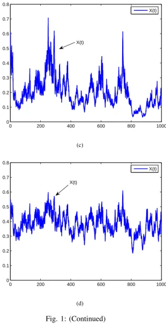
Fig. 1: Solution of Eq.(23). (a) shows that the population goes to extinction (σ1 = 0.65); (b) shows that the population is non-persistent in the mean (σ1=
√
0.4); (c) shows that the population is weakly persistent (σ1= 0.6); (d) indicates that the population is stochastically permanent (σ1= 0.5).
In Fig.1, we choose r0 = 0.32, r1 = 0.5, C0(t) =
0.2 + 0.05 sint, a = 0.1, σ2 = σ3 = 1. The only difference between conditions of Fig.1(a), Fig.1(b), Fig.1(c)
0 200 400 600 800 1000
0 0.1 0.2 0.3 0.4 0.5 0.6 0.7 0.8
X(t)
X(t)
(c)
0 200 400 600 800 1000
0 0.1 0.2 0.3 0.4 0.5 0.6 0.7 0.8
X(t)
X(t)
(d)
Fig. 1: (Continued)
0 50 100 150 200
0.2 0.3 0.4 0.5 0.6 0.7 0.8 0.9 1
x(t) y(t) X(t)
y(t)
0 20 40 60 80 100 0
0.05 0.1 0.15 0.2 0.25 0.3 0.35 0.4
x1(t)
x2(t)
X1(t)
X2(t)
(a)
0 500 1000 1500 2000
0 0.02 0.04 0.06 0.08 0.1
0.12 x1(t)
x2(t)
X1(t)
X2(t)
(b)
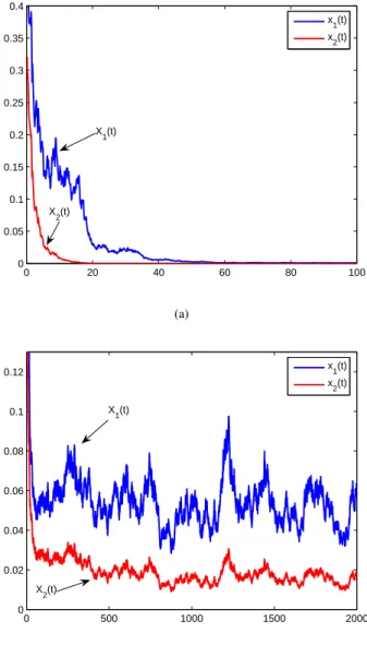
Fig. 3: Solution of Eq.(17). (a) shows that all the populations go to extinction (r10 = 0.08 and r20 = 0.12); (b) shows that Eq.(17) is stochastic permanent (r10 = 0.11andr20=
0.153).
and Fig.1(d) is that the value of σ1 is different. In Fig.1(a), we letσ1= 0.65. Hence
lim sup t→+∞
t−1∫ t 0
b(s)ds=−0.01<0.
In view of Theorem 1, x(t) goes to extinction. Fig.1(a) confirms this. In Fig.1(b), we let σ1 =
√
0.4. Therefore,
lim inf
t→+∞b(t) = 0. It then follows from Theorem 2 that x(t)
is non-persistent in the mean. See Fig.1(b). In Fig.1(c), we choose σ1 = 0.6. Thus lim sup
t→+∞
t−1∫t
0b(s)ds = 0.04 > 0. According to Theorem 3,x(t)is weakly persistent, Fig.1(c) confirms this. In Fig.1(d), we let σ1 = 0.5. Therefore,
lim inf
t→+∞b(t) = 0.025. It then follows from Theorem 4 that
x(t)is stochastic permanent. See Fig.1(d).
In Fig.2, the parameters are same with that in Fig.1(d). Then by Theorem 5, model (3) is globally attractive. Fig.2 confirms this.
Now let us turn to model (17). For the sake of simplicity, we choose n = 2and θij = 1. In Fig.3, we choose r11 =
r21 = 0.5, C0(t) = 0.2, a11 = 0.4, a12 = 0.2, a21 = 0.3,
a22 = 0.4, σ11 = 0.4, σ21 = 0.5, σ113 = σ123 = 0.8,
σ21 = 0.5, σ22 = 0.5, σ213 = σ223 = 0.9. The only difference between conditions of Fig.3(a) and Fig.3(b) is that the values ofr10andr20are different. In Fig.3(a), we choose
r10= 0.08andr20= 0.12. Hence
lim sup t→+∞
t−1∫ t 0
b1(s)ds=−0.005<0,
lim sup t→+∞ t
−1∫ t 0
b2(s)ds=−0.01<0.
By Theorem 6, bothx1andx2go to extinction. See Fig.3(a). In Fig.3(b), we letr10= 0.11andr20= 0.153. Therefore,
lim inf
t→+∞b1(t) = 0.025, lim inft→+∞b2(t) = 0.023.
By Theorem 9, model (17) is stochastic permanent. See Fig.3(b).
VI. CONCLUSION
In this paper, under the assumptions that all the coefficients are affected by white noise, we have proposed and investigat-ed a stochastic single-species Gilpin-Ayala population model in a polluted environment. We have established the sufficient conditions for extinction, non-persistence in the mean, weak persistence and stochastic permanence of the population. The critical value between weak persistence and extinction have been obtained. We have also demonstrated that the solution of the model is globally attractive. Some recent results have been extended and improved.
Our results indicate that a different type of environmental noise has a different effect on the persistence and extinction of the species (see Remark 1). By the definition of b(t), the white noise σ1B˙1(t) is unfavorable for the persistence of the population, the white noise σ2B˙2(t) has no impact on the persistence or extinction of the population, the white noiseσ3B˙3(t)is also unfavorable for the persistence of the population.
Our Theorems 1-4 have some important and interesting bi-ological meanings. From Theorems 1 and 3 one can observe that persistence and extinction of the populationx(t)depend only on the growth rate r0, the power of the white noises
σ2
1 andσ23, the dose-response parameter of the population to the organismal toxicant concentration r1, the concentration of toxicant in the organism C0(t), but are independent of initial population sizex0, the parametersθanda, as well as the power of the white noiseσ2
2. So in order to conserve a species, one has the following ways.
(i) To reduce the values ofσ2
1 andσ32.
(ii) To reduce the concentration of toxicant in the organism (i.e., to reduce the pollutant output u(t)).
However, one could not conserve a population by influencing σ2
2 andθ.
ACKNOWLEDGMENT
The authors thank the anonymous referee for those helpful comments and valuable suggestions. The authors also thank Dr. Hong Qiu for helping us to improve the English exposi-tion.
REFERENCES
[1] T. G. Hallam, C. E. Clark and R. R. Lassider, “Effects of toxicant on population: a qualitative approach I. Equilibrium environmental exposure,”Ecological Modelling, vol. 8, no.3, pp. 291-304, 1983. [2] T. G. Hallam, C. E. Clark and G. S. Jordan, “Effects of toxicant on
population: a qualitative approach II. First Order Kinetics,”Journal of Mathematical Biology, vol. 109, no. 1, pp. 411-429, 1983.
[3] T. G. Hallam and J. L. Deluna, “Effects of toxicant on populations: a qualitative approach III. Environmental and food chain pathways,” Journal of Theoretical Biology, vol. 109, no. 3, pp. 411-429, 1984. [4] T. G. Hallam and Z. Ma, “Persistence in population models with
demographic fluctuations,”Journal of Mathematical Biology, vol. 24, no. 3, pp. 327-339, 1986.
[5] Z. Ma. B. Song and T. G. Hallam, “The threshold of survival for systems in a fluctuating environment,”Bulletin of Mathematical Biology, vol. 51, no. 3, pp. 311-323, 1989.
[6] Z. Ma, G. Cui and W. Wang, “Persistence and extinction of a population in a polluted environment,”Mathematical Biosciences, vol. 101, no. 1, pp. 75-97, 1990.
[7] H. I. Freedman and J. B. Shukla, “Models for the effect of toxicant in single-species and predator-prey systems,”Journal of Mathematical Biology, vol. 30, no. 1, pp. 15-30, 1991.
[8] W. Wang and Z. Ma, “Permanence of populations in a polluted environment,”Mathematical Biosciences, vol. 122, no. 2, pp. 235-248, 1994.
[9] B. Buonomo, A. D. Liddo and I. Sgura, “A diffusive-convective model for the dynamics of population-toxicant intentions: Some analytical and numerical results,”Mathematical Biosciences, vol. 157, no. 2, pp. 37-64, 1999.
[10] P. D. N. Srinivasu, “Control of environmental pollution to conserve a population,”Nonlinear Analysis: Real World Applications, vol. 3, no. 3, pp. 397-411, 2002.
[11] J.He and K.Wang, “The survival analysis for a population in a polluted environment,”Nonlinear Analysis: Real World Applications, vol. 10, no. 3, pp. 1555–1571, 2009.
[12] H. Liu and Z. Ma, “The threshold of survival for system of two species in a polluted environment,”Journal of Mathematical Biology, vol. 30, no. 1, pp. 49-51, 1991.
[13] Z. Ma, W. Zong and Z. Luo, “The thresholds of survival for an n-dimensional food chain model in a polluted environment,”Journal of Mathematical Analysis and Applications, vol. 210, no. 2, pp. 440-458, 1997.
[14] J. Pan, Z. Jin and Z. Ma, “Thresholds of survival for an n-dimensional Volterra mutualistic system in a polluted environment,” Journal of Mathematical Analysis and Applications, vol. 252, no. 2, pp. 519-531, 2000.
[15] B. Liu, L. Chen and Y. Zhang, “The effects of impulsive toxicant input on a population in a polluted environment,”Journal of Biological Systems, vol. 11, no. 3, pp. 265-274, 2003.
[16] B. Liu, Z. Teng and L. Chen, “The effects of impulsive toxicant input on two-species Lotka-Volterra competition system,”International Journal of Information & Systems Sciences, vol. 1, no. 2, pp. 207-220, 2005.
[17] J. Jiao, W. Long and L.Chen, “A single stage-structured population model with mature individuals in a polluted environment and pulse input of environmental toxin,”Nonlinear Analysis: Real World Applications, vol. 10, no. 5, pp. 3073-3081, 2009.
[18] Z. Li and F. Chen, “Extinction in periodic competitive stage-structured Lotka-Volterra model with the effects of toxic substances,”Journal of Computational and Applied Mathematics, vol. 231, no. 1, pp. 143-153, 2009.
[19] R. M. May, Stability and Complexity in Model Ecosystems, USA: Princeton University Press, 2001.
[20] T.C.Gard, “Stochastic models for toxicant-stressed populations,” Bul-letin of Mathematical Biology, vol. 54, no. 5, pp. 827–837, 1992. [21] M.Liu and K.Wang, “Survival analysis of stochastic single-species
population models in polluted environments,” Ecological Modelling, vol. 220, no. 9, pp. 1347-1357, 2009.
[22] M.Liu and K.Wang, “Persistence and extinction of a stochastic single-specie model under regime switching in a polluted environment,” Journal of Theoretical Biology, vol. 264, no. 3, pp. 934–944, 2010.
[23] M.Liu, K.Wang and Q.Wu, “Survival analysis of stochastic competitive models in a polluted environment and stochastic competitive exclusion principle,”Bulletin of Mathematical Biology, vol. 73, no. 9, pp. 1969-2012, 2011.
[24] M.Liu and K.Wang, “Survival analysis of a stochastic cooperation system in a polluted environment,”Journal of Biological Systems, vol. 19, no. 2, pp. 183-204, 2011.
[25] M.Liu and K.Wang, “Persistence and extinction of a single-species population system in a polluted environment with random perturbations and impulsive toxicant input,”Chaos, Solitons & Fractals, vol. 45, no. 12, pp. 1541-1550, 2012.
[26] M.Liu and K.Wang, “Dynamics of a non-autonomous stochastic Gilpin-Ayala model,”Journal of Applied Mathematics and Computing, vol. 43, no. 1-2, pp. 351-368, 2013.
[27] M.E.Gilpin and F.G.Ayala, “Global models of growth and competi-tion,”Proceedings of the National Academy of Sciences of the United States of America, vol. 70, no. 3, pp. 3590-3593, 1973.
[28] X.R.Mao, G.Marion and E.Renshaw, “Environmental Brownian noise suppresses explosions in populations dynamics,”Stochastic Processes and their Applications, vol. 97, no. 1, pp. 95-110, 2002.
[29] D.Q Jiang, N.Z. Shi and X.Y. Li, “Global stability and stochastic permanence of a non-autonomous logistic equation with random pertur-bation,”Journal of Mathematical Analysis and Applications, vol. 340, no. 1, pp. 588-597, 2008.
[30] X.R.Mao,Stochastic Differential Equations and Applications, English: Horwood Publishing, 1997.
[31] Q.Luo and X.R.Mao, “Stochastic population dynamics under regime switching,” Journal of Mathematical Analysis and Applications, vol. 334, no. 1, pp. 69-84, 2007.
[32] I.Barbalat, “Systems dequations differentielles d’osci d’oscillations nonlineaires,”Revue Roumaine de Mathematiques Pures et Appliquees, vol. 4, no. 2, pp. 267–270, 1959.
[33] D.J.Higham, “An algorithmic introduction to numerical simulation of stochastic differential equations.”SIAM Review, vol. 43, no. 3, pp. 525– 546, 2001.
[34] F.H.Shekarabi, M. Khodabin and K. Maleknejad, “The Petrov-Galerkin method for numerical solution of stochastic Volterra integral equations”, IAENG International Journal of Applied Mathematics, vol. 44, no. 4, pp. 170-176, 2014.
[35] D. Jana, S. Chakraborty and N. Bairagi, “Stability, nonlinear oscil-lations and bifurcation in a delay-induced predator-prey system with harvesting,”Engineering Letters, vol. 20, no. 3, pp. 238-246, 2013. [36] C.Xu, Y.Wu and L.Lu, “On permanence and asymptotically periodic
solution of a delayed three-level food chain model with Beddington-DeAngelis functional response,”IAENG International Journal of Ap-plied Mathematics, vol. 44, no. 4, pp. 163-169, 2014.
[37] K.Du, G.Liu and G.Gu, “A class of control variates for pricing asian options under stochastic volatility models”, IAENG International Journal of Applied Mathematics, vol. 43, no. 2, pp. 45-53, 2013. [38] K.Du, G.Liu and G.Gu, “Accelerating Monte Carlo method for pricing