A Multi-Stage Optimization Model With Minimum Energy Consumption-Wireless Mesh Networks

(1)

A Multi-Stage Optimization Model With Minimum

Energy Consumption-Wireless Mesh Networks

S.Krishnakumar

Research Scholar, CSE Dept., SRM University

Chennai, India

Dr.R.Srinivasan

CSE Dept, SRM University

Chennai, India

Abstract—Optimization models related with routing, bandwidth utilization and power consumption are developed in the wireless mesh computing environment using the operations research techniques such as maximal flow model, transshipment model and minimax optimizing algorithm. The Path creation algorithm is used to find the multiple paths from source to destination.A multi-stage optimization model is developed by combining the multi-path optimization model, optimization model in capacity utilization and energy optimization model and minimax optimizing algorithm. The input to the multi-stage optimization model is a network with many source and destination. The optimal solution obtained from this model is a minimum energy consuming path from source to destination along with the maximum data rate over each link. The performance is evaluated by comparing the data rate values of superimposed algorithm and minimax optimizing algorithm. The main advantage of this model is the reduction of traffic congestion in the network.

Keywords-optimization; breakthrough; transportation; aximization; superimposed; transshipment.

I. INTRODUCTION

A. Formulation of Linear programming problem (LPP)

Let s be the source node and N be a set of neighbor nodes of source. Let xij be the rate of transmission of packets over the link (i,j) and cij be the capacity of the link (i,j). Then LPP form of maximal flow problem is

Maximize sj

N j

x



 It represents the amount of flow

passing from the source to the sink. Subject to the constraints

jk k ij j

x





For all j (flow conservation

condition)

(Total incoming flow = Total outgoing flow) xij cij (capacity constraint)

xij 0 (non-negativity restrictions)

Even though this LPP can be solved using simplex method, we are using a simple and efficient algorithm called maximal flow algorithm [20] to find the maximal flow.

1) Maximal Flow Algorithm

Step 1: For all links set the residual capacity equal to the initial capacity and label source node 1 with [, -]. Set i = 1 and go to step 2.

Step 2:Determine Si as the set unlabeled nodes j that can be reached directly from mode i by arcs with positive residuals. If Si is non-empty go to Step 3 otherwise go to Step 4

Step 3: Determine k in Si such that Cik = max {Cij} where j belongs to Si and Cij represents capacity of the link (i,j). Set Ak = Cik and label node k with (Ak, i). If the sink node has been labeled (i.e., k = n) and a breakthrough path is found, go to step 5. Otherwise, set i=k, and go to step 2.

Step 4: (Backtracking)If i=1, no further breakthroughs are possible; go to step 6. Otherwise, let r be the node that has been labeled immediately before the current node i and remove i from the nodes that are adjacent to r. Set i = r, and go to step 2.

Step 5:(determination of residue network). Let Np = [1, k1, k2….., n) define the nodes of the path breakthrough path from source 1 to sink n. Then the maximum flow along the path is computed as

Fp = min {A1, Ak1, Ak2…An}.

The residual capacity of each arc along the breakthrough path is decreased by Fp in the direction of the flow and increased by Fp in the reverse direction. Reinstate any nodes that were removed in step 4. Set i = 1, and return to step 2 to attempt a new breakthrough path.

Step 6: (Solution)

(a) Given that m breakthrough paths have been determined, compute the maximal flow in the network as F = F1 + F2+……..+Fm

(b) The optimal flow over the link (i,j) is computed as follows:

(2)

Figure1: Maximum Flow Algorithm

II. OPTIMIZATION MODEL FOR CAPACITY UTILIZATION Using Shannon’s theorem, we can calculate capacity of a

link from its bandwidth. We assume that the nodes have infinite energy to transmit any number of packets in order to estimate the maximum data rate over each link. Then we apply maximal flow algorithm to find the maximum rate of transmission of packets over each link and the maximal flow in the network.

A. Input

1. A network with source and destination 2. Capacity of each link in the network.

B. Procedure

Maximal flow algorithm

C. Output

1. Maximum number of packets that can be transmitted from source in one second.

2. Maximum rate of transmission of packets over each link. Maximum flow algorithm for many sources and many destinations:

A maximal flow problem may have several sources and sinks. The objective is to find the maximum flow between the number of sources and destinations. We can reduce the problem of determining a maximal flow in a network with multiple sources and multiple sinks to an ordinary maximal flow problem [2, 5, and 7].

Figure 2: Many sources to many destinations

Firstly, we are converting this multiple sources and multiple sinks into only one source and one destination. For

this, We are creating two nodes as Super source(S’) and Super Destination(D’),then adding the edge(S’,Si) with capacity C(S’,Si)=MAX The MAX value is the maximum capacity of

all the links or infinite capacity will be allocated as the capacity (link) of the super source and the super destination. Then we are connecting such that all the source nodes are get connected with the Super source and all the destination nodes are get connected with the Super destination [3, 17]. Now this situation is assumed as the data passed form single source and destination. Then we can implement the maximum flow algorithm.

Figure2.1: Superimposed Sources and destinations

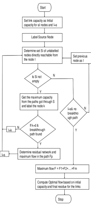
SUPERIMPOSED ALGORITHM: Y Y N N Y N Start

Set link capacity as Initial capacity for al nodes and I=s

Label Source Node

Determine set Si of unlabelled nodes directly reachable from the node I

Is Si not empty

Get the maximum capacity from the paths got through S and label the node k

If k=d & breakthrough path found

Determine residual network and maximum flow in the path Fp

I=s& no breakthro ugh path

Set previous node as I

I=k

I=s

Maximum flow F = F1+F2+….+Fm

Compute Optimal flow based on initial capacity and final residue for the links

Stop Y Y N N Y N Start

Set link capacity as Initial capacity for al nodes and I=s

Label Source Node

Determine set Si of unlabelled nodes directly reachable from the node I

Is Si not empty

Get the maximum capacity from the paths got through S and label the node k

If k=d & breakthrough path found

Determine residual network and maximum flow in the path Fp

I=s& no breakthro ugh path

Set previous node as I

I=k

I=s

Maximum flow F = F1+F2+….+Fm

Compute Optimal flow based on initial capacity and final residue for the links

(3)

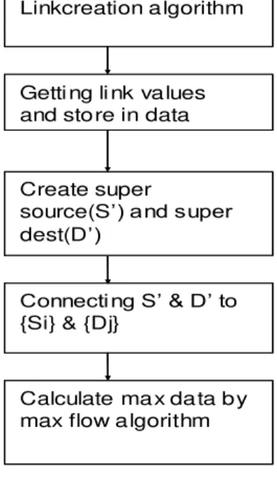
Step 1: creating the links for the network randomly by the input .The links will be generated as N * N link matrix in

which 1’s and 0’s will be generated where '1' denotes link existence and ‘0’ non- existence of links.

Step 2: Randomly generating link capacity for the created links and storing in data

Step3: creating two nodes as Super source(S’) and Super

Destination (D’), then adding the edge(S’, Si) with capacity C(S’, Si) =MAX

Step4: Implement The Maximum Flow Algorithm.

Figure 2.2: Finding break paths

III. TRANSPORTATION MODEL

Let there be m source nodes and n destination nodes. Let Si be a supply from node i and dj be a demand from node j. Let cij be the energy required to transmit a packet from node i to node j and xij be the number of packets that can be transmitted from node i to node j. Let Pi be the power level of node i.

Objective of transportation problem is to minimize the total energy consumption given by

ij

n

j

m

i

x

c





1

Subject to the constraints

xij + xi2 + ………+ xin = Si ; i=1, ……….,m (supply constraint)

xij + x2j + ………+ xmj = dj ; j=1, ………,m (demand constraint)

j cij xij Pi for all i (power constraint) And

xij 0 for all i and j

Procedure for Solving Transportation Problem:

A. MODI Method (Modified Distribution Method) [20]

Cell:Each cell represents a shipping route, which is an arc on the network and a decision variable in the Linear Programming formulation.

Step 1 Formulate the transportation table

Step 2 Construct the initial basic feasible solution by using any of the following methods

(i) NWC rule

(ii) LCM

(iii) VAM

To get the optimal solution (with smaller number of iterations) quickly, use VAM.

Step 3 Test the optimality

Make sure that there are m+n-1 non-zero allocations (Non-degenerate basic feasible solution). These allocations should be in independent positions.

(i) Determine ui i=1…m vj j=1…n

Such that for each occupied cell (r,s) crs = ur + vs

This can be done by choosing arbitrarily one of the ui = 0 or vj = 0. For more convenience, choose the row with the most allocations. If ith row has the most allocations (among rows) then take ui = 0.

(ii) Calculate the cell evaluations (net evaluations)

ij = cij – (ui + vj ) for all unoccupied cells (empty cells).

Note that ij = 0 if (i,j) is an occupied cell. (iii) If ij 0, then the present solution is optimal.

(iv) If at least one ij 0n for at least one cell then the present solution is not optimal.

Step 4 (Iteration towards optimal solution)

(i) Choose the cell which has the most negative ijvalue and mark * in it (The corresponding variable is entering non-basic variable)

(ii) Draw a closed path consisting of horizontal and vertical lines beginning and ending at * cell and having its corners at the allocated cells.

Mark + sign at * cell and + and – signs alternatively at other corner cells of the path. The cell with + signs are called donor cells, which has the least allocation in the leaving basic variable.

(iii) Add the value of leaving basic variable to the allocation for each recipient cell. Subtract this value from the allocation for each donor cell.

Linkcreation algorithm

Calculate max data by max flow algorithm Create super

source(S’) and super

dest(D’)

Connecting S’ & D’ to

{Si} & {Dj}

Getti ng li nk values and store in data Linkcreation algorithm

Calculate max data by max flow algorithm Create super

source(S’) and super

dest(D’)

Connecting S’ & D’ to

{Si} & {Dj}

(4)

This gives improved feasible solution to step 3 for testing optimality.

Remark

In Step 4, (i) if the entering non-basic variable has a tie, then select a variable which has lower cost i.e., if ij and rs are most negative, then select (i,j) cell, if cij is small.

B. Unbalanced transportation problem

A transportation problem is said to be unbalanced if the total supply is not equal to total demand.

SOLUTION TO THE UNBALANCED TRANSPORTATION PROBLEM Convert the unbalanced transportation problem into a balanced transportation problem by the following techniques. (i) Total supply > Total demand (Surplus of supply)

Add a dummy destination node to distribute the surplus (excess) amount of supply and let zero be the cost of transportation to this dummy destination.

i.e., add a dummy column at end of the transportation table and take the excess amount of supply (Total supply – Total demand) as the demand at this destination. Take zero as the unit transportation cost for the cells in this column.

(ii) Total supply < total demand (Slackness or Supply)

Add a dummy source node to produce the slackness of supply in order to saturate excess amount of demand i.e., Add a dummy row at the end of the transportation table. Supply at the dummy source = Total demand – Total supply. Take zero as the unit transportation cost for the cells in this row.

C. Maximization Type Transportation Problem

A maximization type transportation problem can be converted into usual minimization type transportation problem by subtracting each of the costs from the highest cost given in the problem to obtain only the optimal solution. For calculating the total transportations cost, use the original cost given in the problem.

D. Transshipment Model

A transportation problem in which the supply may not be sent directly from sources to destinations, i.e., the supply may pass through one or more sources or destinations before reaching its actual destination, is called as transshipment problem.

The nodes of network with both input and output links act as both sources and destinations, and are referred to as transshipment nodes. The remaining nodes are either pure supply nodes or pure demand nodes. The transshipment model can be converted into a transportation model by computing the amount of supply and demand at different nodes as follows:

Figure: 3 Flowchart for solving a Transportation Model

Let P = total supply (or demand)

Supply at a pure supply node = Original supply Supply at a transshipment node = Original supply + P Demand at a pure demand node = Original Demand Demand at a transshipment node = Original Demand + P Assume that transportation cost (energy consumption) the same node is zero i.e., cii = 0 for all i.

E. Energy Optimization Model

(5)

Let e be the energy required by a host to transmit a message to another host who is d distance away. Then e = rdc where r and c are constants for the specific wireless mesh system. Hence energy consumption is proportional to the distance between nodes. Here distance between nodes is calculated by number of hops between the nodes.

Here supply at a node is the number of packets that can be transmitted by a node and demand is the number of packets that can be received by a node. Hence, supply and demand at a node are depending on the available battery energy in the node.

We assume that transshipment nodes (i.e., nodes forwarding packets) possess sufficient energy to forward packets. We can apply transshipment model to get minimum energy consuming path and the maximum number of data that can be transmitted.

1) Input

a) A network with source and destination

b) Residual power level at each node

c) Distance between nodes

2) Procedure

Transshipment model algorithm

3) Output

a) Minimum energy consuming path

b) Maximum number of packets that can be transmitted

c) Total energy consumption.

IV. OPTIMIZATION

We consider a wireless network containing multiple sources and multiple destinations. In this chapter we discuss about the multistage optimization model which is a combination of the data rate and energy optimization that have been developed in the earlier sections.

The objective of this model to find the minimum energy consuming path from source to destination and the maximum data rate over each link in the minimum energy consuming path[2,3,7]

Transmission of messages is continued along minimum energy consuming path for a period of time T. The parameter T can be determined using the time taken by the nodes for recharging their battery and dynamically changing speed of topology of the network

A. Minimax optimizing algorithm:

The Minimax algorithm is the algorithm for integrating the maximization and minimization [2, 7 and 17]. In this algorithm, the maximization (maximal flow model) is compared with the minimization (transshipment algorithm) and the break paths are selected and calculating the maximum data rate with minimum energy consumption.

ALGORITHM:

Step 1: creating the links for the network randomly by the input .The links will be generated as N * N link matrix in

which 1’s and 0’s will be generated where '1' denotes link

existence and ‘0’ non-existence of links.

Step 2: Randomly generating link capacity for the created links and storing in data and tempdata and getting the Sources {Si} and Destinations {Dj} from the input.

Step 3: Calculate the maximum Data rate through superimposed algorithm.

Step 4: Check whether the iterations are complete for source and destination {SDij}, then go to step9 or go to step 5. Step 5: If there is any path, calculate the maximum data rate using maximal flow algorithm in tempdata or go to step 7. Step 6: Send the path (links) to the transshipment algorithm and get the energy E {SDij} consumed in that path. Go to step 5.

Step 7: Select the Break paths with energy based on data rate.

Step 8: Update the value in data and update data value to temp data.

Step 9: Calculate the total data rate of each {SDij}. Step 10: Compare the data rate values of superimposed algorithm and the Minimax Algorithm and plot it in graph.

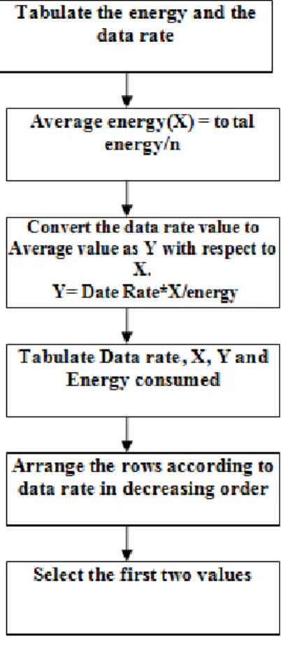
Selecting Break paths:

Step 1: Tabulate the energy and the data rate of each path for each source and destination {SDij}.

Step 2: Calculate average energy as X, where n is the number of nodes.

Step 3: Convert the data rate value to Average value as Y and tabulate it.

Step 4: Arrange the rows according to data rate, in decreasing order.

Step 5: Select the first two paths. V. RESULTS Experiment Inputs-Number of nodes : 11 Number of sources and

Destination {Si, Dj} :3, 4 Source Nodes {si} : 2, 3, 4 Destination Nodes {dj} : 5, 6, 7,8.

Paths {Pij} : 25, 26, 28, 36, 37, 45, 47

Input: no of nodes, {Si, Dj {si},{dj},{Pij}.

(6)

Figure 4: Minimax optimizing algorithm

VI. COMPARISON:

Analysis of performance of the model by comparing the simulation results of this Minmax model with the simulation results of superimposed algorithm related with power consumption and Bandwidth utilization in the Wireless environment. Packet loss attribute is not included for this model, as it occurs in both the models

A. 1. Superimposed algorithm data rate value and Minimax

optimizing algorithm data rate value with respect to number of nodes:

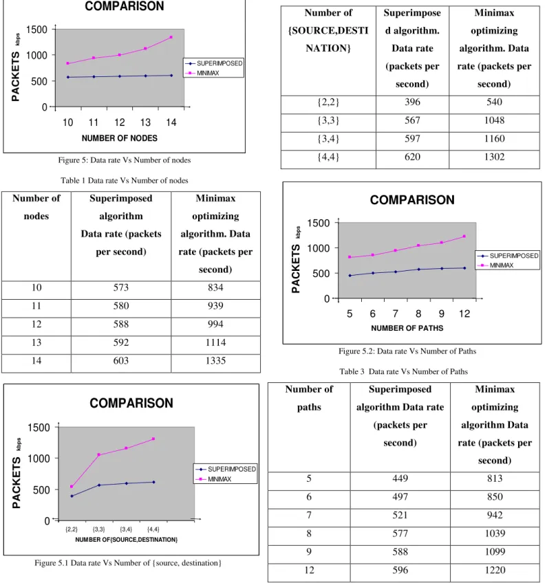
In the figure 5, we are comparing the values of superimposed algorithm data rate value and Minimax optimizing algorithm data rate value with respect to number of nodes. For the increase in number of nodes, the data rate value of both the algorithm is increased.

Figure 4.1: Selecting Break paths:

But the data rate value of Minimax optimizing algorithm is greater than the superimposed algorithm.

B. Superimposed algorithm data rate value and Minimax

optimizing algorithm data rate value with respect to number of sources and destinations:

In the figure 5.1, we are comparing the values of superimposed algorithm data rate value and Minimax optimizing algorithm data rate value with respect to number of sources and destinations.

For the increase in number of sources and destinations, the data rate value of both the algorithm is increased. But the data rate value of Minimax optimizing algorithm is greater than the superimposed algorithm.

C. Superimposed algorithm data rate value and Minimax

optimizing algorithm data rate value with respect to number of paths:

In the figure 5.2, we are comparing the values of superimposed algorithm data rate value and Minimax optimizing algorithm data rate value with respect to number of paths.

For the increase in number of paths, the data rate value of both the algorithm is increased. But the data rate value of Minimax optimizing algorithm is greater than the superimposed algorithm

N Y

links links

{Si}&{Dj}

Linkcreation algorithm Max flow for {Si}

&{Dj}(overall)

Sending to transhipment algorithm

Calculating energy for SDij

Selecting B paths with energy based on data rate

For all paths{pij}}

For each Si &Dj Superimposed

Algorithm

Compare the two values

Plot the graph based on the result.

Calculate the total data of each - SDij

Subtracting in data & copy to temp data

If SDij=0

Data Temp Data Maximum flow

algorithm Getting link values and store in data & tempdata

Temp Data

N Y

links links

{Si}&{Dj}

Linkcreation algorithm Max flow for {Si}

&{Dj}(overall)

Sending to transhipment algorithm

Calculating energy for SDij

Selecting B paths with energy based on data rate

For all paths{pij}}

For each Si &Dj Superimposed

Algorithm

Compare the two values

Plot the graph based on the result.

Calculate the total data of each - SDij

Subtracting in data & copy to temp data

If SDij=0

Data Temp Data Maximum flow

algorithm Getting link values and store in data & tempdata

(7)

Figure 5: Data rate Vs Number of nodes

Table 1 Data rate Vs Number of nodes

Number of

nodes

Superimposed

algorithm

Data rate (packets

per second)

Minimax

optimizing

algorithm. Data

rate (packets per

second)

10 573 834

11 580 939

12 588 994

13 592 1114

14 603 1335

Figure 5.1 Data rate Vs Number of {source, destination}

Table 2 Data rate Vs Number of {source, destination}

Number of

{SOURCE,DESTI

NATION}

Superimpose

d algorithm.

Data rate

(packets per

second)

Minimax

optimizing

algorithm. Data

second)

{2,2} 396 540

{3,3} 567 1048

{3,4} 597 1160

{4,4} 620 1302

Figure 5.2: Data rate Vs Number of Paths

Table 3 Data rate Vs Number of Paths

Number of

paths

Superimposed

algorithm Data rate

(packets per

second)

Minimax

optimizing

algorithm Data

second)

5 449 813

6 497 850

7 521 942

8 577 1039

9 588 1099

12 596 1220

COMPARISON

0 500 1000 1500

10 11 12 13 14

NUMBER OF NODES

P

AC

KE

T

S

kbp

s

SUPERIMPOSED MINIMAX

COMPARISON

0 500 1000 1500

{2,2} {3,3} {3,4} {4,4}

NUMBER OF{SOURCE,DESTINATION}

P

AC

KE

T

S

k

bp

s

SUPERIMPOSED MINIMAX

COMPARISON

0 500 1000 1500

5 6 7 8 9 12

NUMBER OF PATHS

P

AC

KE

T

S

kbp

s

(8)

VII. CONCLUSION

The optimization models related with routing, bandwidth utilization and power consumption are developed using the OR techniques like maximal flow algorithm, transshipment model and minimax optimizing algorithm

VIII. SUGGESTIONS FOR FURTHER WORK

1) Determination of frequency of running the model by exploiting the recharging capability of the nodes and the speed of dynamically changing topology of the network.

2) Analysis of performance of the model by comparing the

simulation results of this model with the simulation results of other routing protocols related with power consumption and Bandwidth utilization in the wireless mesh computing environment.

3) The comparison metrics, with other existing

methodologies, other parameters and with more

demonstration.

REFERENCES

[1] R.Ahuja, T. Magnati and J. Orlin, (1993), “Network Flows Theory, Algorithms and Applications”, Prentice Hall, Upper Saddle River, N.J. [2] Thomas H.cormen, Charles E.leiserson, Ronald L.rivest,(2001),

“Introduction to Algorithms”,3rd_{ed., Prentice Hall, New Delhi.} [3] N. Bambos (June 1998), “Toward Power-sensitive Network

Architectures in Wireless Communications: Concepts, Issues, and

Design Aspects”, IEEE Personal Communications Magazine, pp. 50-59. [4] M. Bazaraa, J. Jarvis, and H. Sherali (1990), “Linear Programming and

Network Flow”, 2nd_{ed., Wiley, New York.}

[5] Benjie Chen, Kyle Jamieson, Hari Balakrishnan, and Robert Morris (July

2001), “Span: An energy-efficient coordination algorithm for topology

maintenance in ad hoc wireless networks”, in 7th Annual Int. Conf.

Mobile Computing and Networking 2001, Rome, Italy.

[6] D. Bertsekas, R. Gallager (2000), “Data Networks”, 2nd_{ed, Prentice Hall} of India, New Delhi.

[7] Philips, Solberg, Ravindran (1976), “Operation Research – techniques

and Practice” ,John Wilen & sons, New York.

[8] B. Brumitt (Oct 2000), “Ubiquitous computing and the roles of Geometry”, IEEE Pers. Commun.pp 47-53.

[9] J.-H. Chang and L. Tassiulas (Sept. 1999), “Routing for maximum system lifetime in wireless ad-hoc networks,” in Proceedings of 37-th Annual Conference on Communication, Control, and Computing, Monticello, II.

[10] J-H Chang and L. Tassiulas (March 2000). “Energy Conserving Routing in Wireless Ad-hoc Networks.” Proceedings of IEEE Infocom 2000. Tel Aviv, Israel.

[11] A. Croll, E. Packman (2001), “Managing Bandwidth”, Pearson Education Asia.

[12] K. Edwards and Rebecca Grinter (September 2001), “At Home with

Ubiquitous Computing: Seven Challenges”, Ubiquitous Computing 2001, Atlanta, GA.

[13] J.M. Rabaey (2001), “Wireless beyond the 3rd_{generation facing the}

energy challenge”, proc. 2001 Int’s symp. Lower power electronics and

design (ISLPED 01), ACM Press, New York, PP 1-3.

[14] T.S. Rappaport (1996), “Wireless Communications: Principles and

practice”, prentice Hall, New Hersey.

[15] V. Rodoplu, et al (June 1998), “Minimum energy mobile wireless

networks”, Proceedings of IEEE ICC, Atlanta, GA, Vol.3, PP 1633 -1639.

[16] M. Satyanarayanan (Aug 2001), “Pervasive Computing: Vision and

Challenges”, IEEE Pers. Commun., PP 10-17.