ACPD
8, 15997–16025, 2008Ship emitted NO2 in the Indian Ocean
K. Franke et al.
Title Page
Abstract Introduction
Conclusions References
Tables Figures
◭ ◮
◭ ◮
Back Close
Full Screen / Esc
Printer-friendly Version
Interactive Discussion Atmos. Chem. Phys. Discuss., 8, 15997–16025, 2008
www.atmos-chem-phys-discuss.net/8/15997/2008/ © Author(s) 2008. This work is distributed under the Creative Commons Attribution 3.0 License.
Atmospheric Chemistry and Physics Discussions
This discussion paper is/has been under review for the journalAtmospheric Chemistry and Physics (ACP). Please refer to the corresponding final paper inACPif available.
Ship emitted NO
2
in the Indian Ocean:
comparison of model results with satellite
data
K. Franke1,2, A. Richter1, H. Bovensmann1, V. Eyring2, P. J ¨ockel3, and J. P. Burrows1
1
University of Bremen, Institute for Environmental Physics, Bremen, Germany
2
Deutsches Zentrum f ¨ur Luft- und Raumfahrt, Institut f ¨ur Physik der Atmosph ¨are, Oberpfaffenhofen, Germany
3
Max Planck Institute for Chemistry, Mainz, Germany
Received: 25 July 2008 – Accepted: 29 July 2008 – Published: 21 August 2008
Correspondence to: K. Franke ([email protected])
ACPD
8, 15997–16025, 2008Ship emitted NO2 in the Indian Ocean
K. Franke et al.
Title Page
Abstract Introduction
Conclusions References
Tables Figures
◭ ◮
◭ ◮
Back Close
Full Screen / Esc
Printer-friendly Version
Interactive Discussion
Abstract
An inventory of NOxemission from international shipping has been evaluated by com-paring NO2tropospheric columns derived from the satellite instruments SCIAMACHY (January 2003 to February 2008), GOME (January 1996 to June 2003), and GOME-2 (March 2007 to February 2008) to NO2columns calculated with the atmospheric chem-5
istry general circulation model ECHAM5/MESSy1 (January 2000 to October 2005). The data set from SCIAMACHY yields the first monthly analysis of ship induced NO2 enhancements in the Indian Ocean. For both data and model consistently the tropo-spheric excess method was used to obtain mean NO2columns over the shipping lane from India to Indonesia, and over two ship free regions, the Bay of Bengal and the cen-10
tral Indian Ocean. In general, the model simulates the differences between the regions affected by ship pollution and ship free regions reasonably well. Minor discrepancies between model results and satellite data were identified during biomass burning sea-sons in March to May over India and the Indochinese Peninsula and August to October over Indonesia. We conclude that the NOxship emission inventory used in this study is 15
a good approximation of NOxship emissions in the Indian Ocean for the years 2002 to 2007. It assumes that around 6 Tg(N) yr−1 are emitted by international shipping glob-ally, resulting in 90 Gg(N) yr−1 in the region of interest when using Automated Mutual Assistance Vessel Rescue System (AMVER) or 72 Gg(N) yr−1when using the Interna-tional Comprehensive Ocean-Atmosphere Data Set (ICOADS) as spatial proxy. The 20
results do not support some previously published lower ship emissions estimates of 3– 4 Tg(N) yr−1 globally, making this study the first that evaluates atmospheric response to NOx ship emission estimates from space.
1 Introduction
Since the industrial revolution the amount of freight transported by international ship-25
ACPD
8, 15997–16025, 2008Ship emitted NO2 in the Indian Ocean
K. Franke et al.
Title Page
Abstract Introduction
Conclusions References
Tables Figures
◭ ◮
◭ ◮
Back Close
Full Screen / Esc
Printer-friendly Version
Interactive Discussion anthropogenic burden of air pollutants. One important pollutant emitted by ships is
ni-trogen monoxide (NO). In the atmosphere NO reacts with ozone (O3) to form nitrogen dioxide (NO2). The sum of NO and NO2, which is known as NOx, is pseudo conserved. As NOx participates in the catalytic production of tropospheric ozone, accurate knowl-edge of amount and distribution of NOx is needed to understand and assess the role 5
of ship emissions on tropospheric composition and climate. Recent estimates of the global NOx emissions from international shipping vary over a large range. The global emission data base EDGAR3.2 includes data for 1995 (Olivier and Berdowsky, 2001), which if scaled to year 2000 values assuming a growth rate of 1.5% yr−1, results in annual NOx emissions of 3.10 Tg(N), similar to the emission totals published by Cor-10
bett et al. (1999) and Endresen et al. (2003). Later estimates vary from 5.93 Tg(N) yr−1 (Corbett and Koehler, 2003) to 6.36 Tg(N) yr−1 (Eyring et al., 2005) for year 2000. In addition to uncertainties in global emission totals, the knowledge of the spatial dis-tribution is limited. As pointed out by Wang et al. (2008), ship activity patterns es-timated by the International Comprehensive Ocean-Atmosphere Data Set (ICOADS) 15
and the Automated Mutual-assistance Vessel Rescue System (AMVER) data set have different spatial and statistical sampling biases. Using these or similar NOx shipping inventories, models have simulated and investigated the impact of shipping emission on tropospheric ozone (Lawrence and Crutzen, 1999; Kasibhatla et al., 2000; Eyring et al., 2007). Using the EDGAR3.2 dataset, the study by Eyring et al. (2007) shows 20
maximum contributions from shipping to annual mean near-surface O3over the North Atlantic (56 ppbv in 2000).
Ship emissions of NOx have been detected in the marine boundary layer (MBL) in satellite data (Richter et al., 2004; Beirle et al., 2004). These studies showed that the NO2enhancement in the shipping lane in the north-eastern Indian Ocean and the Red 25
ACPD
8, 15997–16025, 2008Ship emitted NO2 in the Indian Ocean
K. Franke et al.
Title Page
Abstract Introduction
Conclusions References
Tables Figures
◭ ◮
◭ ◮
Back Close
Full Screen / Esc
Printer-friendly Version
Interactive Discussion from seasonal changes in the pollutant distribution. Both studies concluded that
rea-sonable agreement exists between the estimate of emissions made using satellite data and that available from emission inventories. However, it is clear that the estimation of lifetime of NOxis one significant source of uncertainty in this comparison.
An alternative approach to investigate the consistency of emission inventories with 5
NO2 measurements is to calculate the column or concentration of NOx levels with at-mospheric chemistry models. Kasibhatla et al. (2000) and Davis et al. (2001) used ship emission totals of 3 Tg(N) yr−1 in global chemistry models and compared them to airborne measurements. They conclude that there is an overestimation of ship in-duced NOx in the models and attribute this to the coarse resolution of the models and 10
the uncertainties in the inventories. Eyring et al. (2007) compared the model output of eight global models at the local time of SCIAMACHY overpass to the satellite data of Richter et al. (2004). Although the geographical pattern of tropospheric NO2is well re-produced, modelled values of the tropospheric column are higher than those observed by SCIAMACHY over the ocean. The shipping lane in the Indian Ocean is not resolved 15
in these simulations because of the low horizontal resolution in the models (between 5.6
◦
×5.6
◦ and 2
.8
◦
×2.8
◦) compared to the satellite data (30
×60 km2, i.e. 0.27
◦
×0.54
◦
at the equator). The study also compares the NO2 total tropospheric columns to the SCIAMACHY observations without applying the tropospheric excess method to the model output. It has been shown by Lauer et al. (2002) that these two quantities differ. 20
The goal of this work is a quantitative assessment of the various NOxship emission estimates that have been published so far. This is achieved by comparing an extended set of satellite NO2 data with results of the atmospheric chemistry general circulation model ECHAM5/MESSy1. In order to have a consistent comparison of modeled and measured NO2 columns, the NO2 tropospheric excess column has been generated 25
ACPD
8, 15997–16025, 2008Ship emitted NO2 in the Indian Ocean
K. Franke et al.
Title Page
Abstract Introduction
Conclusions References
Tables Figures
◭ ◮
◭ ◮
Back Close
Full Screen / Esc
Printer-friendly Version
Interactive Discussion are analysed and the knowledge of the emissions inventories for the Indian Ocean
investigated.
2 Data retrieval and analysis
2.1 Tropospheric NO2columns retrieved from space
The tropospheric NO2 columns are retrieved from measurements of the upwelling so-5
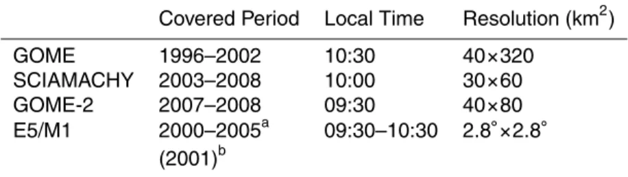
lar radiation in nadir viewing geometry by the three spectrometers GOME (Burrows et al., 1999; Richter and Burrows, 2002), SCIAMACHY (Burrows et al., 1995; Bovens-mann et al., 1999; Richter et al., 2004), and GOME-2 (which is a somewhat improved Version of GOME, Callies et al., 2000), which fly on board the satellites ERS-2, EN-VISAT, and METOP-A, respectively. These satellites are in sun synchronous orbits 10
having equator crossing times of 10:30 a.m., 10:00 a.m., and 09:30 a.m., respectively. GOME provides global data from 1996 to June 2003 having a spatial resolution of 40×320 km2 and 40×80 km2. Data from January 2003 to February 2008 for SCIA-MACHY having a spatial resolution of 30×60 km2 and from March 2007 to February
2008 for GOME-2 (40×80 km2) are available. Monthly mean values were calculated on
15
a grid of 0.125◦
×0.125◦. Table 1 describes some relevant instrumental parameters.
The retrieval approach used to determine NO2 column from the nadir measure-ments by the satellite instrumeasure-ments is based on the Differential Optical Absorption Spec-troscopy (DOAS) method. This technique determines the NO2 slant column density, SCD, along the light path through the atmosphere in the spectral window between 425 20
and 450 nm by separating high frequency molecular signatures from broadband ab-sorption and scattering (Brewer et al., 1973; Noxon, 1975; Platt et al., 1979). In order to retrieve tropospheric amounts of NO2the technique known as tropospheric excess method (TEM) has been employed. This relies on the longitudinal homogeneity of the stratospheric column. Comparison of the measurements at a given location with the 25
tropo-ACPD
8, 15997–16025, 2008Ship emitted NO2 in the Indian Ocean
K. Franke et al.
Title Page
Abstract Introduction
Conclusions References
Tables Figures
◭ ◮
◭ ◮
Back Close
Full Screen / Esc
Printer-friendly Version
Interactive Discussion spheric excess SCD. This approach assumes implicitly that tropospheric amount of
NO2in this reference region is negligible (Fig. 1). The SCD can be converted to a verti-cal column density (VCD) by division with an Air Mass Factor (AMF). The AMF corrects for the different sensitivity of measurements to absorption in different altitudes, which is determined by the relative penetration depth and depends on the magnitude of the 5
surface spectral reflectance and multiple scattering within the atmosphere. This is of particular importance for absorbers located close to the surface. The resulting tropo-spheric excess column is denoted as TEC. This method belongs to a family of retrieval approaches called residual techniques. The analysis used is described in Richter et al. (2004), more detailed descriptions of the retrieval method can be found in Richter and 10
Burrows (2002) and in Burrows et al. (1999). The overall accuracy of the retrieved columns is about 34% (Richter et al., 2004).
2.2 Model description
ECHAM5/MESSy1 (hereafter referenced as E5/M1) is an Atmospheric Chemistry Gen-eral Circulation Model (AC-GCM) (J ¨ockel et al., 2006). The applied spectral resolution 15
is T42, corresponding to a quadratic-gaussian grid of approximately 2.8◦×2.8◦ in
lon-gitude and latitude, respectively. The used model setup has 90 layers on a hybrid-pressure grid reaching up to 0.01 hPa. Details of the E5/M1 simulation S1 that is used in this study are described in J ¨ockel et al. (2006). In order to be able to directly com-pare the model results with observations, the model dynamics has been nudged using 20
operational analysis data from the European Centre for Medium-Range Weather Fore-casts (ECMWF) from January 2000 to October 2005. The model integration time-step is 900 s. Output has been archived as 5-hourly instantaneous fields. This yields an hourly resolved diurnal cycle within 5 days of integration.
Anthropogenic and natural emissions of NO, CO, SO2, NH3 and several hydrocar-25
bon species are taken from the EDGAR3.2FT20001dataset (Olivier et al., 2005). NOx 1
ACPD
8, 15997–16025, 2008Ship emitted NO2 in the Indian Ocean
K. Franke et al.
Title Page
Abstract Introduction
Conclusions References
Tables Figures
◭ ◮
◭ ◮
Back Close
Full Screen / Esc
Printer-friendly Version
Interactive Discussion emissions include anthropogenic sources with an annual emission rate of 31 Tg(N) and
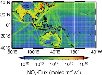
biomass burning emissions with an annual emission rate of 9.3 Tg(N) (see electronic supplement to Pozzer et al., 2007)2. The contribution of ship emission to total anthro-pogenic NOx emissions is 6.3 Tg(N) yr−1, which are spatially distributed according to the AMVER activity pattern (Eyring et al., 2005). For comparison with satellite data the 5
relevant E5/M1 parameters are given in Table 1. The E5/M1 model has been evalu-ated by comparison to the compiled tropospheric in-situ observations of Emmons et al. (2000) 3 and other observational data. These show that the model simulates tropo-spheric distributions of NO, HNO3 and PAN concentrations over the tropical Ocean reasonably well (J ¨ockel et al., 2006).
10
As a result of the model output being provided at full hours in universal time for every grid box and the ENVISAT satellite having a local equator crossing time of 10:00 am, the model data between 09:30 a.m. and 10:30 a.m. have been averaged in the regions of the ship emissions and the respective reference sectors. Furthermore, to reduce the effects of the inter-annual variability, a 6 year climatological average (2000–2005) of 15
the model data has been used. Two techniques are applied to derive the tropospheric NO2 columns from the model output. The first technique is consistent with the TEM employed for satellite data. The total columns are derived by vertically integrating over all layers of the atmosphere. NO2TECs are then calculated by subtracting the mean total column at the same latitude in a reference sector over the Pacific from the total 20
column at a given location. These NO2columns are hereafter denoted as E5/M1(TEM). In the second approach, the column is calculated by integrating the NO2 amount over the lowest 20 model layers (approx. up to 200 hPa) and denoted as E5/M1(SUM).
2
http://www.atmos-chem-phys.net/7/2527/2007/acp-7-2527-2007-supplement.pdf
3
ACPD
8, 15997–16025, 2008Ship emitted NO2 in the Indian Ocean
K. Franke et al.
Title Page
Abstract Introduction
Conclusions References
Tables Figures
◭ ◮
◭ ◮
Back Close
Full Screen / Esc
Printer-friendly Version
Interactive Discussion
3 Results and discussion
3.1 Comparison of model and SCIAMACHY data
The shipping lane from the southern tip of the Indian subcontinent to Indonesia in the north eastern Indian Ocean has been selected to verify ship induced NOx, because here ship traffic is concentrated in a narrow line and other local NOx emissions are 5
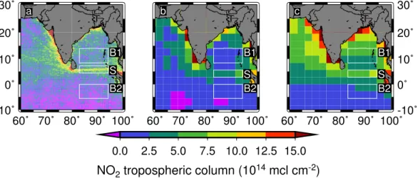
negligible. For a quantitative comparison of the model results and the satellite data three regions (S, B1, and B2) depicted in Fig. 2 are defined. The region S is the region which contains the shipping lane. The region B1 is north of the shipping lane and the region B2 is south of the lane. The regions B1 and B2 are assumed not to be signifi-cantly influenced by emissions from shipping. All regions have a longitudinal width of 10
four model grid boxes from 83◦E to 94.2◦E. The regions B1 and B2 have a latitudinal width of two model boxes: B1 extending from 8.4◦N to 14◦N and B2 from 5.6◦S to the equator. The position of the modelled shipping lane (Fig. 2b) is shifted relative to the observed shipping lane (see below). Therefore the region S is defined as the grid box extending from 2.8◦N to 5.6◦N. For the satellite data, the region S has a latitudinal width 15
of 2.8◦ centred around the maximum of the NO
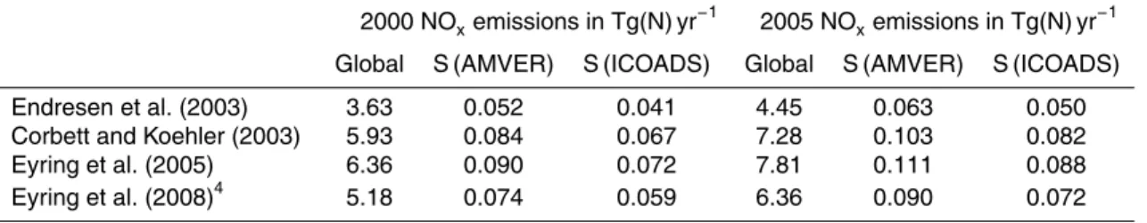
2enhancement in the given month, as shown by the white line in Fig. 3. NOx ship emissions in region S are calculated from the global emission totals of Endresen et al. (2003), Corbett and Koehler (2003) and Eyring et al. (2005, 20084) using ship activity patterns from AMVER and ICOADS, see Table 2. In the region S the emissions range from 41 Gg(N) yr−1(Endresen et al., 2003 20
with ICOADS) to 90 Gg(N) yr−1(Eyring et al., 2005 with AMVER), i.e. depending on the inventory the emission estimate differ by more than a factor of 2.
In Fig. 2, the mean February NO2 tropospheric column amount, derived from all available SCIAMACHY measurements between 2003 and 2008 is compared to E5/M1
4
ACPD
8, 15997–16025, 2008Ship emitted NO2 in the Indian Ocean
K. Franke et al.
Title Page
Abstract Introduction
Conclusions References
Tables Figures
◭ ◮
◭ ◮
Back Close
Full Screen / Esc
Printer-friendly Version
Interactive Discussion (TEM) and E5/M1 (SUM). The shipping lane in the satellite data is identified by the
region having NO2TEC of 10×1014molec cm−2 in comparison to the surrounding re-gion, where values of around 2×10¹⁴molec cm−2are found. The width of the shipping lane is approximately 1◦ latitude or 110 km (Fig. 2a).
While the overall agreement with E5/M1 (TEM) data is good, the coarse horizontal 5
resolution of the model becomes apparent (Fig. 2b). As the shipping lane is close to a latitudinal boundary of the model grid cells, the shipping signature in the model data is shifted southward relative to the satellite measurements. Qualitatively, as the model grid box is approximately twice as large as the width of the measured shipping lane the maximum reduces from 10×1014molec cm−2to 5×10¹⁴molec cm−2.
10
The difference between E5/M1 (TEM) and E5/M1 (SUM) is about 2.5×10¹⁴molec cm−2, with the satellite data being in better agreement with the E5/M1 (TEM) data. While Fig. 2 only shows February, this is valid for all months. This underlines the importance of choosing a consistent data analysis method for the comparison of model and satellite data. In the following analysis only E5/M1 (TEM) is 15
used.
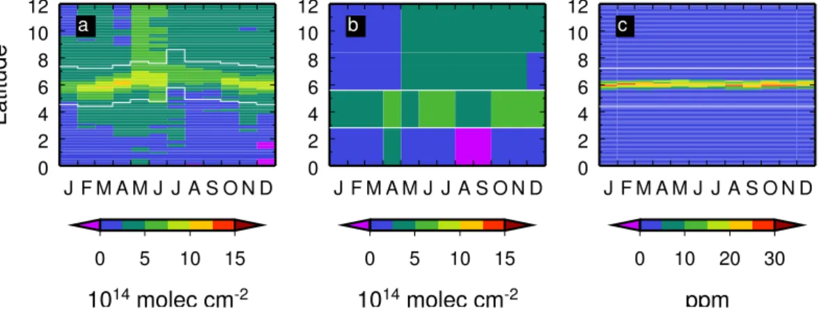
Figure 3 compares zonal mean (83◦E to 94.2◦E) NO
2 TEC derived from SCIA-MACHY to E5/M1 (TEM) and the AMVER ship activity pattern as a function of time and latitude. The shipping lane is discernible by enhanced values of NO2TEC throughout the year in the satellite data (Fig. 3a). However, the latitudinal position of the maximum 20
enhancement varies over the year, being further south in the northern hemispheric winter months and further north in the summer. Additionally, the width of the shipping lane and the magnitude of TEC changes over the year. In January and from July to September the signature of ship emissions on the NO2 TECs spreads over a larger area and the maximum is less pronounced, never rising above 7.5×10¹⁴molec cm−2. 25
pat-ACPD
8, 15997–16025, 2008Ship emitted NO2 in the Indian Ocean
K. Franke et al.
Title Page
Abstract Introduction
Conclusions References
Tables Figures
◭ ◮
◭ ◮
Back Close
Full Screen / Esc
Printer-friendly Version
Interactive Discussion terns over this region. In the summer the wind comes mainly from the south whereas
in winter it comes from the north. This seasonal variation was also observed by Beirle et al. (2004) in GOME data. The correlation of the latitude of the maximal NO2 TEC with the mean meridional wind derived from ECMWF reanalysis data is 0.75, i.e. a rea-sonable strong correlation. In addition, in the satellite data of NO2 TEC, a significant 5
seasonality over the Bay of Bengal north of the shipping lane between 8◦N and 12◦N is observed in the months May and June. The potential sources of this behaviour are discussed below.
3.2 Analysis of NO2TEC from the three different instruments
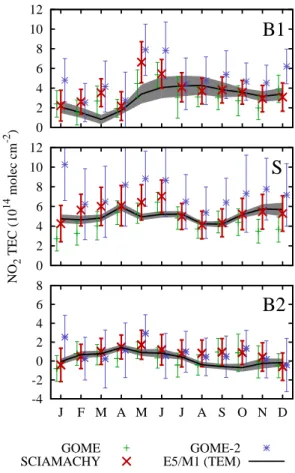
Figure 4 shows the mean NO2 tropospheric excess column for three different instru-10
ments compared to the model output in the selected regions S, B1, and B2. For each month the mean of all available years has been calculated from GOME (8 years), SCIA-MACHY (5 years), GOME-2 (1 year), and E5/M1 data (6 years). The standard deviation of the averaged data comprises instrument noise plus atmospheric variability of NO2 and is depicted as errorbar in Fig. 4. As the local time of model data in the regions 15
is centred around 10:00 LT the most direct comparison is between SCIAMACHY and E5/M1(TEM), reducing potential differences through diurnal variations in NOx. In gen-eral SCIAMACHY and E5/M1 (TEM) are in good agreement. In region B1 SCIAMACHY is somewhat higher than E5/M1 (TEM) in March and May, while in region B2 SCIA-MACHY is somewhat higher than E5/M1 (TEM) in September and October. The small 20
discrepancies in region B1 and B2 coincide with the biomass burning seasons in adja-cent landmasses as seen in the TRMM Fire Index5, i.e. typically February to May/June in India and the Indochinese Peninsula and from August to October in Indonesia. As the EDGAR3.2FT2000 dataset is valid for the year 2000 and SCIAMACHY measure-ments are from 2003 to 2008 discrepancies between model input and actual biomass 25
burning emissions can be expected.
5
ACPD
8, 15997–16025, 2008Ship emitted NO2 in the Indian Ocean
K. Franke et al.
Title Page
Abstract Introduction
Conclusions References
Tables Figures
◭ ◮
◭ ◮
Back Close
Full Screen / Esc
Printer-friendly Version
Interactive Discussion The GOME and GOME-2 measurements are consistent with SCIAMACHY data
within errorbars in the regions S, B1, and B2 throughout the year. One exception is the large value of GOME-2 in January 2008. As the NO2 TEC measured by SCIA-MACHY in January 2008 is also enhanced in comparison to former years (not shown), we concider this to be a result of a special situation occurring in this month. As this 5
deviation happens in all three regions, it is considered not to be related to the ship traf-fic and is not further discussed in this study. The observation of enhanced NO2 TEC by all three instruments compared to model results in region B1 in March and May and in region B2 in September and October indicates that they do not result from a bias inherent to SCIAMACHY, but reflect variations in tropospheric NO2content.
10
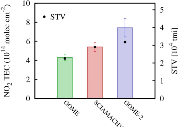
While monthly means among the satellite instruments are consistent within error-bars, the annual mean NO2 TEC over the regions S among the instruments differ (Fig. 5). Possible explanations of this difference in TEC NO2over region S are
(i) changes of ship emissions over time,
(ii) diurnal variation of NO2, 15
(iii) change of background NOx field.
In the following we will discuss these aspects in more detail.
(i) Over the last 30 years a clear and well understood correspondence is observed between fuel consumption and seaborne trade in ton miles, because the work done in global trade is proportional to the energy required (Eyring et al., 20084). The to-20
tal seaborne trade volume (STV) has risen from 20 968 tmi (tonne miles) in 1996 to 31 847 tmi in 2007 (Fearnleys, 2007). As no significant measures of NOx-reductions have been introduced, we use the increase in STV over this period as an indicator for NOxincrease. The rise in STV over the time period covered by GOME measurements (1996–2002) is 15% with a mean STV of 22 549 tmi, while it is a 21% increase with 25
ACPD
8, 15997–16025, 2008Ship emitted NO2 in the Indian Ocean
K. Franke et al.
Title Page
Abstract Introduction
Conclusions References
Tables Figures
◭ ◮
◭ ◮
Back Close
Full Screen / Esc
Printer-friendly Version
Interactive Discussion than the mean STV for GOME observations, while it is 10% lower than the mean STV
of 31 847 tmi during the time period of GOME-2 measurements (2007–2008).
In order to assess the difference in the measurements that is due to the raise in NOx emissions, linear regression on the monthly mean NO2 TECs (this time with-out inter-annual average) was performed. Linear regression over 84 months of 5
GOME measurements in region S yields a slope of (0.0±0.13)×1014molec cm−2yr−1,
which corresponds to (0±22)% of the mean NO2 TEC of all available GOME data. For the 67 month of SCIAMACHY measurements the regression gives a slope of (0.15±0.15)×1014molec cm−2yr−1 (14±14%). This implies that no significant trend
is discernible within the error of measurement over the periods of measurements of 10
either GOME or SCIAMACHY. However, the change in mean NO2 TEC between the measurement periods of GOME and SCIAMACHY has increased by (26±15)%, which
is in agreement with the rise of 29% in STV (Fig. 5). On the other hand, the mean NO2 TEC as observed by GOME-2 from 2007 to 2008 is (37±22)% higher than the
mean NO2TEC over the period of measurement of SCIAMACHY (2003–2008), which 15
is substantially higher than what would be expected from the 10% rise of the mean STV.
(ii) The diurnal variation of NO2 arises from variation of its photodissociation rate and the effective first order removal rate for its reaction with OH. As a result of these two processes NO2 decreases during the morning. As the equator crossing times of 20
GOME-2, SCIAMACHY and GOME are 09:30, 10:00, and 10:30 LT, respectively, the in-struments see different parts of this diurnal cycle. To investigate whether the observed differences can be explained by the diurnal cycle, the mean NO2 TECs from GOME and SCIAMACHY are compared for the period August 2002 to June 2003 and for the period March 2007 to February 2008 for SCIAMACHY and GOME-2. By confining the 25
ACPD
8, 15997–16025, 2008Ship emitted NO2 in the Indian Ocean
K. Franke et al.
Title Page
Abstract Introduction
Conclusions References
Tables Figures
◭ ◮
◭ ◮
Back Close
Full Screen / Esc
Printer-friendly Version
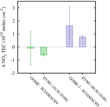
Interactive Discussion Over the region S the model predicts a decrease in mean NO2 TEC of 0.6–
0.7×10¹⁴molec cm−2 over the half of an hour between the respective equator
cross-ing times (Fig. 6). However, the difference in mean NO2 TEC derived from GOME and SCIAMACHY measurements from 2002/2003 show no significant decrease over this half hour (green data in Fig. 6). On the other hand, the difference in 5
mean NO2 TEC measured by GOME-2 and SCIAMACHY in 2007/2008 is about (1.6±1.4)×1014molec cm−2 in region S, and therefore greater than predicted by the
model (blue data in Fig. 6). In conclusion, the differences among the three satellite instruments cannot be explained by the diurnal variaion, as the difference between GOME and SCIAMACHY that measure at 10:30 a.m. and 10:00 a.m. repsectively is 10
smaller than expected from the model while the difference between SCIAMACHY and GOME-2 (09:30 a.m.) is larger.
In conclusion of this section, the different satellite instruments measure different mean NO2TECs over region S. While the difference between GOME and SCIAMACHY is consistent with the rise in STV, no diurnal variation could be identified in the time pe-15
riod of overlapping measurements of GOME and SCIAMACHY. On the other hand, the difference in NO2 TEC between GOME-2 and SCIAMACHY is greater than expected from either diurnal variation of NO2or rise in NOx ship emissions. Another explanation could be a change in background NOx levels due to a change of outflow of NOx from adjacent landmasses (Kunhikrishnan and Lawrence, 2004). As a detailed assessment 20
of these influences from adjacent landmasses requires additional data of continental sources and also is not related to the main topic of this paper on ship induced NO2 changes over the Indian Ocean it is not further pursued.
3.3 Evaluation of ship emission inventories
So far we could show that the model agrees reasonably well with the satellite data. 25
ACPD
8, 15997–16025, 2008Ship emitted NO2 in the Indian Ocean
K. Franke et al.
Title Page
Abstract Introduction
Conclusions References
Tables Figures
◭ ◮
◭ ◮
Back Close
Full Screen / Esc
Printer-friendly Version
Interactive Discussion background regions B1 and B2 is determined, to see if there is a significant
over-estimation of ship induced NOx in the model simulation. Overestimation could result because in the model simulation one of the higher NOxestimates for international ship-ping has been used (see Table 2 for comparison), and because plume processing has been neglected, which could lead to different NOx lifetimes inside the plume (Franke 5
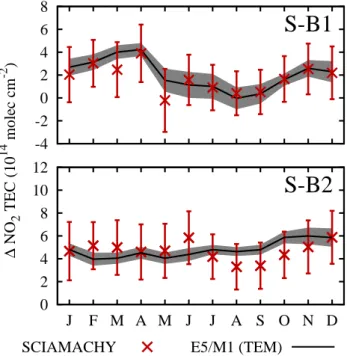
et al., 2008). However, the model results and the measurements agree well in the difference between regions S and B1 with the exception of May (Fig. 7, upper panel). This has its origin in the high value in B1 in this month (Fig. 4) and is therefore not related to ship emissions. Differences between S and B1 show an annual cycle with a minimum of 0.5×10¹⁴molec cm−2 in August and a maximum of 4×10¹⁴molec cm−2
10
in April. The correlation between the two curves is 0.87 (0.95 excluding May). The difference between S and B2 shows no significant annual cycle, and the model results and the satellite data are close to 5×10¹⁴molec cm−2(Fig. 7, lower panel).
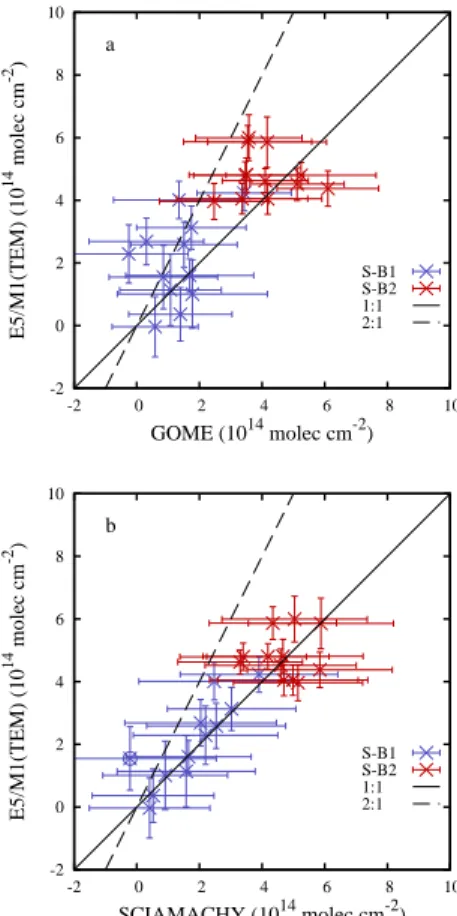
The agreement between model results and satellite data is more obvious in Fig. 8. Here the differences in NO2 TEC between the regions from model output are plotted 15
against those from GOME and SCIAMACHY. SCIAMACHY values for S-B1 are all (with the exception of the May value) located near the 1:1 line showing again the high corre-lation and also the absence of a significant bias. The S-B2 differences centre also on the bisecting line, showing no discernable correlation, but also no bias (Fig. 8, lower panel). On the other side, GOME values are slightly lower, being left of the 1:1 line. 20
The ship inventory by Eyring et al. (2005) applied in the model simulation results in emission totals of 90 Gg(N) yr−1in region S. As discussed earlier, other emission inven-tories give around half of this amount even if scaled with the increase of total seaborne trade to the year 2005, see Table 2. If we assume linear relation between simulated NO2 and emitted NOx as a simple approximation, with half the NOx emissions the 25
ACPD
8, 15997–16025, 2008Ship emitted NO2 in the Indian Ocean
K. Franke et al.
Title Page
Abstract Introduction
Conclusions References
Tables Figures
◭ ◮
◭ ◮
Back Close
Full Screen / Esc
Printer-friendly Version
Interactive Discussion with either AMVER or ICOADS are too low in comparison to the satellite data.
4 Conclusions
Ship emissions of NOx in the Indian Ocean have been analysed with the help of measurements from GOME (1996–2002), SCIAMACHY (2003–2007), and GOME-2 (2007/2008) in comparison to a global model simulation. The Differential Optical Ab-5
sorption Spectroscopy (DOAS) method and the tropospheric excess method (TEM) were used to retrieve NO2 tropospheric excess columns (TECs) in the northern Indian Ocean. The satellite data was compared to NO2 TEC retrieved from the output of a nudged simulation with the atmospheric chemistry general circulation model ECHAM5/MESSy1 (2000–2005). The shipping route from India to Indone-10
sia can be detected in satellite data with an enhancement in NO2 TEC of about 8×10¹⁴molec cm−2. A monthly variation of the latitudinal position of the NO
2 enhance-ment could be identified with a correlation of 0.75 between the latitudinal position of the maximal NO2 enhancement and mean meridional wind speed derived from ECMWF reanalysis data.
15
For detailed analysis three regions were defined, one including the shipping lane (S), one in the Bay of Bengal (B1) and one over the free Indian Ocean (B2). B1 and B2 are assumed not to be influenced by ship emissions. Overall comparison of SCIAMACHY NO2 TEC and E5/M1 TEC in the defined regions shows good agreement with SCIA-MACHY being somewhat higher in B2 in August to November and somewhat higher 20
in S and B1 in March and May. These differences in NO2TEC coincide with biomass burning seasons on landmasses nearby, i.e. February to May over India and the In-dochinese Peninsula and August to October over Indonesia.
An analysis of differences between mean NO2 TEC values in region S shows that GOME-2 has a (2±1)×1014molec cm−2 higher TEC than SCIAMACHY. In
25
er-ACPD
8, 15997–16025, 2008Ship emitted NO2 in the Indian Ocean
K. Franke et al.
Title Page
Abstract Introduction
Conclusions References
Tables Figures
◭ ◮
◭ ◮
Back Close
Full Screen / Esc
Printer-friendly Version
Interactive Discussion ences were analysed: First, the diurnal cycle of NO2as the three instruments measure
NO2at slightly different times during the day (GOME-2 at 09:30 a.m.; SCIAMACHY at 10:00 a.m.; GOME at 10:30 a.m.), and second, the change in NOxship emissions over the measurement period. The diurnal variation could not unambiguously identified in the satellite data, because the standard deviation of the measurements is greater than 5
the change in NO2 TEC as calculated by the model. Some of the difference can be attributed to the difference in the measurement period as ship emissions in the ship-ping lanes from 1996 to 2007 are expected to have increased. Linear Regression has been used to study the trend in NO2 TEC within the measurement period from either GOME or SCIAMACHY. For this trend analysis no significant change greater than the 10
standard deviation could be identified. However, the difference of (26±15)% in mean
NO2 TEC between satellite measurements by GOME and SCIAMACHY is consistent with the rise of 29% in mean seaborne trade volume.
Finally, the ship induced NO2enhancement was derived from the difference between NO2 TEC in the ship influenced region S and the ship free regions B1 and B2. Here, 15
agreement between satellite data and model results is very good with a correlation of 0.87. In addition, a simple linear estimation of results expected from using emis-sion data with half the NOx flux give significantly lower estimations of ship induced change in NO2 TEC over the Indian Ocean. Therefore we conclude, that a ship emis-sion inventory with around 6 Tg(N) yr−1globally resulting in around 90 Gg(N) yr−1in the 20
region of interest when using the Automated-Mutual-Assistance Vessel Rescue Sys-tem (AMVER) or around 72 Gg(N) yr−1 when using the International Comprehensive Ocean-Atmosphere Data Set (ICOADS) as spatial proxy provides better agreement with measurement in the Indian Ocean than previously published lower ship emissions estimates of 3–4 Tg(N) yr−1globally. A more extensive comparison of the ship emission 25
inventories on the global scale would be necessary to further strengthen this result.
ACPD
8, 15997–16025, 2008Ship emitted NO2 in the Indian Ocean
K. Franke et al.
Title Page
Abstract Introduction
Conclusions References
Tables Figures
◭ ◮
◭ ◮
Back Close
Full Screen / Esc
Printer-friendly Version
Interactive Discussion and State of Bremen and the EU ACCENT network. We would like to thank Ulrike Burkhardt
for her comments on the manuscript.
References
Beirle, S., Platt, U., von Glasow, R., Wenig, M., and Wagner, T.: Estimate of nitrogen ox-ide emissions from shipping by satellite remote sensing, Geophys. Res. Lett., 31, L18102,
5
doi:10.1029/2004GL020312, 2004. 15999, 16006
Bovensmann, H., Burrows, J., Buchwitz, M., Frerick, J., No ¨el, S., Rozanov, V., Chance, K., and Goede, A.: SCIAMACHY: Mission Objectives and Measurement Modes, J. Atmos. Sci., 56, 127–150, 1999. 16001
Brewer, A., McElroy, C., and Kerr, J.: Nitrogen dioxide concentrations in the atmosphere,
Na-10
ture, 246, 129–133, 1973. 16001
Burrows, J., H ¨olzle, E., Goede, A., Visser, H., and Fricke, W.: SCIAMACHY—scanning imaging absorption spectrometer for atmospheric chartography, Acta Astronaut., 35, 445–451, 1995. 16001
Burrows, J., Weber, M., Buchwitz, M., et al.: The Global Ozone Monitoring Experiment (GOME):
15
Mission Concept and First Scientific Results, J. Atmos. Sci., 56, 151–175, 1999. 16001, 16002
Callies, J., Corpaccioli, E., Eisinger, M., Hahne, A., and Lefebvre, A.: GOME-2- Metop’s second-generation sensor for operational ozone monitoring, ESA Bull., 102, 28–36, 2000. 16001
20
Corbett, J., Fischbeck, P., and Pandis, S.: Global nitrogen and sulfur inventories for oceangoing ships, J. Geophys. Res., 104, 3457–3470, 1999. 15999
Corbett, J. J. and Koehler, H. W.: Updated emissions from ocean shipping, J. Geophys. Res., 108, 4650, 2003. 15999, 16004, 16017
Davis, D., Grodzinsky, G., Kasibhatla, P., Crawford, J., Chen, G., Liu, S., Bandy, A., Thornton,
25
D., Guan, H., and Sandholm, S.: Impact of ship emissions on marine boundary layer NOx
and SO2distributions over the Pacific basin, Geophys. Res. Lett., 28, 235–238, 2001. 16000
Emmons, L., Hauglustaine, D., Mueller, J., Carroll, M., Brasseur, G., Brunner, D., Staehelin, J., Thouret, V., and Marenco, A.: Data composites of airborne observations of tropospheric ozone and its precursors, J. Geophys. Res., 105, 20 497–20 538, 2000. 16003
ACPD
8, 15997–16025, 2008Ship emitted NO2 in the Indian Ocean
K. Franke et al.
Title Page
Abstract Introduction
Conclusions References
Tables Figures
◭ ◮
◭ ◮
Back Close
Full Screen / Esc
Printer-friendly Version
Interactive Discussion Endresen, Ø., Sørg ˚ard, E., Sundet, J., Dalsøren, S., Isaksen, I., Berglen, T., and Gravir, G.:
Emission from international sea transportation and environmental impact, J. Geophys. Res., 108, 4560, 2003. 15999, 16004, 16017
Eyring, V., K ¨ohler, H. W., van Aardenne, J., and Lauer, A.: Emissions from international ship-ping: 1. The last 50 years, J. Geophys. Res., 110, D17305, doi:10.1029/2004JD005619,
5
2005. 15999, 16003, 16004, 16010, 16016, 16017, 16018
Eyring, V., Stevenson, D. S., Lauer, A., Dentener, F. J., Butler, T., Collins, W. J., Ellingsen, K., Gauss, M., Hauglustaine, D. A., Isaksen, I. S. A., Lawrence, M. G., Richter, A., Rodriguez, J. M., Sanderson, M., Strahan, S. E., Sudo, K., Szopa, S., van Noije, T. P. C., and Wild, O.: Multi-model simulations of the impact of international shipping on Atmospheric Chemistry
10
and Climate in 2000 and 2030, Atmos. Chem. Phys., 7, 757–780, 2007, http://www.atmos-chem-phys.net/7/757/2007/. 15999, 16000
Fearnleys: Fearnleys Review 2007, The Tanker and Bulk Markets and Fleets, Tech. Rep., Oslo, 2007. 16007
Franke, K., Eyring, V., Sander, R., Hendricks, J., Lauer, A., and Sausen, R.: Toward effective
15
emissions of ships in global models, Meteorol. Z., 17, 117–129, 2008. 16010
J ¨ockel, P., Tost, H., Pozzer, A., Br ¨uhl, C., Buchholz, J., Ganzeveld, L., Hoor, P., Kerk-weg, A., Lawrence, M., Sander, R., Steil, B., Stiller, G., Tanarhte, M., Taraborrelli, D., van Aardenne, J., and Lelieveld, J.: The atmospheric chemistry general circulation model ECHAM5/MESSy1: consistent simulation of ozone from the surface to the mesosphere,
20
Atmos. Chem. Phys., 6, 5067–5104, 2006, http://www.atmos-chem-phys.net/6/5067/2006/. 16002, 16003
Kasibhatla, P., Levy, H., Moxim, W., Pandis, S., Corbett, J., Peterson, M., Honrath, R., Frost, G., Knapp, K., Parrish, D., and Ryerson, T.: Do emissions from ships have a significant impact on concentrations of nitrogen oxides in the marine boundary layer?, Geophys. Res. Lett., 27,
25
2229–2232, 2000. 15999, 16000
Kunhikrishnan, T. and Lawrence, M.: Sensitivity of NOx over the Indian Ocean to emissions
from the surrounding continents and nonlinearities in atmospheric chemistry responses, Geophys. Res. Lett., 31, L15109, doi:10.1029/2004GL020210, 2004. 16009
Lauer, A., Dameris, M., Richter, A., and Burrows, J. P.: Tropospheric NO2columns: a compari-30
son between model and retrieved data from GOME measurements, Atmos. Chem. Phys., 2, 67–78, 2002, http://www.atmos-chem-phys.net/2/67/2002/. 16000
photo-ACPD
8, 15997–16025, 2008Ship emitted NO2 in the Indian Ocean
K. Franke et al.
Title Page
Abstract Introduction
Conclusions References
Tables Figures
◭ ◮
◭ ◮
Back Close
Full Screen / Esc
Printer-friendly Version
Interactive Discussion chemistry and climate, Nature, 402, 167–170, 1999. 15999
Noxon, J.: Nitrogen dioxide in the stratosphere and tropsphere as measured by ground-based absoption spectroscopy, Science, 189, 547–549, 1975. 16001
Olivier, J. and Berdowsky, J.: Global emission sources and sinks, in: The Climate System, edited by: Berdowski, J., Guicherit, R., and Heij, B., 33–77, A. A. Balkema Publishers/Swets
5
& Zeitlinger Publishers, Lisse, The Netherlands, 2001. 15999
Olivier, J. G. J., van Aardenne, J. A., Dentener, F., Ganzeveld, L., and Peters, J. A. H. W.: Recent trends in global greenhouse gas emissions: regional trends and spatial distribution of key sources, in: Non-CO2 Greenhouse Gases (NCGG-4), edited by: van Amstel, A., 325–330, Millpress, Rotterdam, ISBN 90 5966 043 9, 2005. 16002
10
Platt, U., Perner, D., and P ¨atz, H.: Simultaneous measurement of atmospheric CH2O, O3, and
NO 2 by differential optical absorption, J. Geophys. Res., 84, 6329–6335, 1979. 16001 Pozzer, A., J ¨ockel, P., Tost, H., Sander, R., Ganzeveld, L., Kerkweg, A., and Lelieveld, J.:
Simulating organic species with the global atmospheric chemistry general circulation model ECHAM5/MESSy1: a comparison of model results with observations, Atmos. Chem. Phys.,
15
7, 2527–2550, 2007, http://www.atmos-chem-phys.net/7/2527/2007/. 16003
Richter, A. and Burrows, J.: Tropospheric NO2 from GOME measurements, Adv. Space Res.,
29, 1673–1683, 2002. 16001, 16002
Richter, A., Eyring, V., Burrows, J., Bovensmann, H., Lauer, A., Sierk, B., and Crutzen, P.: Satellite measurements of NO2from international shipping emissions, Geophys. Res. Lett.,
20
31, L23110, doi:10.1029/2004GL020822, 2004. 15999, 16000, 16001, 16002
Song, C., Chen, G., Hanna, S., Crawford, J., and Davis, D.: Dispersion and chemical evolution of ship plumes in the marine boundary layer: Investigation of O3/NOy/HOx chemistry, J.
Geophys. Res., 108, 4143, doi:10.1029/2002JD002216, 2003. 15999
Wang, C., Corbett, J., and Firestone, J.: Improving Spatial Representation of Global Ship
Emis-25
ACPD
8, 15997–16025, 2008Ship emitted NO2 in the Indian Ocean
K. Franke et al.
Title Page
Abstract Introduction
Conclusions References
Tables Figures
◭ ◮
◭ ◮
Back Close
Full Screen / Esc
Printer-friendly Version
Interactive Discussion
Table 1.Important parameters of the used satellite data and the model.
Covered Period Local Time Resolution (km2)
GOME 1996–2002 10:30 40×320
SCIAMACHY 2003–2008 10:00 30×60
GOME-2 2007–2008 09:30 40×80
E5/M1 2000–2005a 09:30–10:30 2.8◦
×2.8◦
(2001)b
a
Period of used ECMWF data.
b
ACPD
8, 15997–16025, 2008Ship emitted NO2 in the Indian Ocean
K. Franke et al.
Title Page
Abstract Introduction
Conclusions References
Tables Figures
◭ ◮
◭ ◮
Back Close
Full Screen / Esc
Printer-friendly Version
Interactive Discussion
Table 2. NOx ship emissions from existing literature. The table summarizes the global
emis-sion total and the emisemis-sion into region S (83◦E–94.2◦E/4.4◦N–7.2◦N) for di
fferent spatial ship activity patterns (AMVER and ICOADS). Emission rates for 2000 are scaled with the increase of total seaborne trade to the year 2005.
2000 NOxemissions in Tg(N) yr−1
2005 NOxemissions in Tg(N) yr−1
Global S (AMVER) S (ICOADS) Global S (AMVER) S (ICOADS)
Endresen et al. (2003) 3.63 0.052 0.041 4.45 0.063 0.050
Corbett and Koehler (2003) 5.93 0.084 0.067 7.28 0.103 0.082
Eyring et al. (2005) 6.36 0.090 0.072 7.81 0.111 0.088
ACPD
8, 15997–16025, 2008Ship emitted NO2 in the Indian Ocean
K. Franke et al.
Title Page
Abstract Introduction
Conclusions References
Tables Figures
◭ ◮
◭ ◮
Back Close
Full Screen / Esc
Printer-friendly Version
Interactive Discussion
60˚E 100˚E 140˚E 180˚ 140˚W
40˚S 20˚S 0˚ 20˚N 40˚N
1012 1013 1014 1015 1016 NOx-Flux (molec m-2 s-1)
Fig. 1. NOx emissions inventory as used in the model simulation. Estimates are taken from
ACPD
8, 15997–16025, 2008Ship emitted NO2 in the Indian Ocean
K. Franke et al.
Title Page
Abstract Introduction
Conclusions References
Tables Figures
◭ ◮
◭ ◮
Back Close
Full Screen / Esc
Printer-friendly Version
Interactive Discussion B1
S
B2 a
60˚ 70˚ 80˚ 90˚ 100˚ -10˚
0˚ 10˚ 20˚ 30˚
60˚ 70˚ 80˚ 90˚ 100˚
B1
S B2 b
60˚ 70˚ 80˚ 90˚ 100˚-10˚ 0˚ 10˚ 20˚ 30˚
B1
S B2 c
0.0 2.5 5.0 7.5 10.0 12.5 15.0
NO2 tropospheric column (1014 mcl cm-2)
Fig. 2. February mean tropospheric NO2 columns: (a) derived from SCIAMACHY
measure-ments from 2003 to 2008 using the DOAS technique and the tropospheric excess method
(TEM).(b)taken from the E5/M1 model using the TEM.(c)taken from the E5/M1 model
inte-grating the NO2concentration up to approximately 200 hPa (SUM). The white boxes indicate
ACPD
8, 15997–16025, 2008Ship emitted NO2 in the Indian Ocean
K. Franke et al.
Title Page
Abstract Introduction
Conclusions References
Tables Figures
◭ ◮
◭ ◮
Back Close
Full Screen / Esc
Printer-friendly Version
Interactive Discussion 0
2 4 6 8 10 12
Latitude
J F M A M J J A S O N D
a
0 5 10 15
1014 molec cm-2
0 2 4 6 8 10 12
J F M A M J J A S O N D
b
0 5 10 15
1014 molec cm-2
0 2 4 6 8 10 12
J F M A M J J A S O N D
c
0 10 20 30
ppm
Fig. 3. Monthly zonal mean NO2tropospheric excess columns(a)derived from SCIAMACHY
measurements from 2003 to 2008 using the DOAS technique and the tropospheric excess
method (TEM);(b)derived from ECHAM5/MESSy1 model simulations from 2000 to 2005 and
ACPD
8, 15997–16025, 2008Ship emitted NO2 in the Indian Ocean
K. Franke et al.
Title Page
Abstract Introduction
Conclusions References
Tables Figures
◭ ◮
◭ ◮
Back Close
Full Screen / Esc
Printer-friendly Version
Interactive Discussion 0
2 4 6 8 10 12
NO
2
TEC (10
14
molec cm
-2 )
S
02 4 6 8 10 12
B1
-4 -2 0 2 4 6 8
J F M A M J J A S O N D
B2
GOME SCIAMACHY
GOME-2 E5/M1 (TEM)
Fig. 4. Monthly mean NO2 tropospheric column in three selected regions over the Indian
ACPD
8, 15997–16025, 2008Ship emitted NO2 in the Indian Ocean
K. Franke et al.
Title Page
Abstract Introduction
Conclusions References
Tables Figures
◭ ◮
◭ ◮
Back Close
Full Screen / Esc
Printer-friendly Version
Interactive Discussion 0
2 4 6 8 10
0 1 2 3 4 5
NO
2
TEC (10
14
molec cm
-2 )
STV [10
4 tmi]
GOME SCIAMACHY GOME-2
STV
Fig. 5. Multiannual mean NO2 tropospheric excess column (TEC) measured with satellite
ACPD
8, 15997–16025, 2008Ship emitted NO2 in the Indian Ocean
K. Franke et al.
Title Page
Abstract Introduction
Conclusions References
Tables Figures
◭ ◮
◭ ◮
Back Close
Full Screen / Esc
Printer-friendly Version
Interactive Discussion -2
-1 0 1 2 3
∆
NO
2
TEC (10
14 molec cm
-2 )
GOME - SCIAMACHYE5/M1 (10:30-10:00) GOME-2 - SCIAMACHYE5/M1 (09:30-10:00)
Fig. 6.Difference in mean NO2TEC (∆NO2TEC) as a result of diurnal variation in tropospheric
NO2over the region S estimated from satellite measurements compared to the corresponding
∆NO2TEC from model simulations. The differences in NO2TEC between GOME (10:30 a.m.)
and SCIAMACHY (10:00 a.m.) measurements are calculated for the period from August 2002
to June 2003. The differences in NO2TEC between GOME-2 (09:30 a.m.) and SCIAMACHY
ACPD
8, 15997–16025, 2008Ship emitted NO2 in the Indian Ocean
K. Franke et al.
Title Page
Abstract Introduction
Conclusions References
Tables Figures
◭ ◮
◭ ◮
Back Close
Full Screen / Esc
Printer-friendly Version
Interactive Discussion -4
-2 0 2 4 6 8
S-B1
∆
NO
2
TEC (10
14 molec cm
-2 )
0 2 4 6 8 10 12
J F M A M J J A S O N D
S-B2
SCIAMACHY E5/M1 (TEM)
Fig. 7. Difference in NO2tropospheric column over the shipping lane from India to Indonesia
to NO2 over the Bay of Bengal (S-B1) and over the central Indian Ocean (S-B2). Data from
ACPD
8, 15997–16025, 2008Ship emitted NO2 in the Indian Ocean
K. Franke et al.
Title Page
Abstract Introduction
Conclusions References
Tables Figures
◭ ◮
◭ ◮
Back Close
Full Screen / Esc
Printer-friendly Version
Interactive Discussion -2
0 2 4 6 8 10
-2 0 2 4 6 8 10
E5/M1(TEM) (10
14 molec cm -2)
GOME (1014 molec cm-2)
a
S-B1 S-B2 1:1 2:1
-2 0 2 4 6 8 10
-2 0 2 4 6 8 10
E5/M1(TEM) (10
14 molec cm -2)
SCIAMACHY (1014 molec cm-2)
b
S-B1 S-B2 1:1 2:1
Fig. 8. Difference in NO2tropospheric column over the shipping lane from India to Indonesia
to NO2over the Bay of Bengal (S-B1) and over the central Indian Ocean (S-B2). Data from(a)
GOME and(b)SCIAMACHY are correlated to output from the model E5/M1. The SCIAMACHY