Turbulence Kinetic Energy budget during the afternoon transition – Part 2: A simple TKE model

(1)

ACPD

15, 29807–29869, 2015

A simple TKE model

E. Nilsson et al.

Title Page

Abstract Introduction

Conclusions References

Tables Figures

◭ ◮

Back Close

Full Screen / Esc

Printer-friendly Version Interactive Discussion

Discussion

P

a

per

|

Discussion

P

a

per

|

Discussion

P

a

per

|

Discussion

P

a

per

|

Atmos. Chem. Phys. Discuss., 15, 29807–29869, 2015 www.atmos-chem-phys-discuss.net/15/29807/2015/ doi:10.5194/acpd-15-29807-2015

This discussion paper is/has been under review for the journal Atmospheric Chemistry and Physics (ACP). Please refer to the corresponding final paper in ACP if available.

Turbulence Kinetic Energy budget during

the afternoon transition – Part 2: A simple

TKE model

E. Nilsson1,2, M. Lothon1, F. Lohou1, E. Pardyjak3, O. Hartogensis4, and

C. Darbieu1

1

Laboratoire d’Aerologie, University of Toulouse, CNRS, Toulouse, France

2

Department of Earth Sciences, Uppsala University, Uppsala, Sweden

3

Department of Mechanical Engineering, Utah University, Salt Lake City, UT, USA

4

Meteorology and Air Quality Section, Wageningen University, Wageningen, the Netherlands

Received: 11 September 2015 – Accepted: 11 September 2015 – Published: 2 November 2015

Correspondence to: E. Nilsson (erik.nilsson@aero.obs-mip.fr, erik.nilsson@met.uu.se)

(2)

ACPD

15, 29807–29869, 2015

E. Nilsson et al.

Title Page

Tables Figures

◭ ◮

Back Close

Full Screen / Esc

Discussion

P

a

per

|

Discussion

P

a

per

|

Discussion

P

a

per

|

Discussion

P

a

per

|

Abstract

A simple model for turbulence kinetic energy (TKE) and the TKE budget is presented for sheared convective atmospheric conditions based on observations from the Boundary Layer Late Afternoon and Sunset Turbulence (BLLAST) field campaign. It is based on an idealized mixed-layer approximation and a simplified near-surface TKE budget. 5

In this model, the TKE is dependent on four budget terms (turbulent dissipation rate, buoyancy production, shear production and vertical transport of TKE) and only requires measurements of three input available (near-surface buoyancy flux, boundary layer depth and wind speed at one height in the surface layer).

This simple model is shown to reproduce some of the observed variations between 10

the different studied days in terms of near-surface TKE and its decay during the afternoon transition reasonably well. It is subsequently used to systematically study the effects of buoyancy and shear on TKE evolution using idealized constant and time-varying winds during the afternoon transition. From this, we conclude that many different TKE decay rates are possible under time-varying winds and that generalizing 15

the decay with simple scaling laws for near-surface TKE of the form tα may be questionable.

The model’s errors result from the exclusion of processes such as elevated shear production and horizontal advection. The model also produces an overly rapid decay of shear production with height. However, the most influential budget terms governing 20

near-surface TKE in the observed sheared convective boundary layers are included, while only second order factors are neglected. Comparison between modeled and averaged observed estimates of dissipation rate illustrate that the overall behavior of the model is often quite reasonable. Therefore, we use the model to discuss the low turbulence conditions that form first in the upper parts of the boundary layer during 25

(3)

ACPD

15, 29807–29869, 2015

E. Nilsson et al.

Title Page

Tables Figures

◭ ◮

Back Close

Full Screen / Esc

Discussion

P

a

per

|

Discussion

P

a

per

|

Discussion

P

a

per

|

Discussion

P

a

per

|

“pre-residual layer,” which is important in determining the onset conditions for the weak sporadic turbulence that occur in the residual layer once near-surface stratification has become stable.

1 Introduction

The daytime atmospheric boundary layer (ABL) is characterized by unstable 5

stratification, turbulent mixing of momentum, heat, scalars and buoyancy-driven eddies. These large eddies are generated by a strong surface heat flux (Emanuel, 1994) but are also influenced by wind shear. This is apparent near the surface as seen in our companion paper Nilsson et al. (2015), which we will refer to as Part 1.

During the course of any day, the atmospheric boundary layer turbulence will 10

naturally respond to different levels of shear and buoyancy production, directly influencing the level of turbulence kinetic energy (TKE). In addition, transport and dissipation of TKE can change substantially from hour-to-hour as well as on shorter and longer time scales, thereby influencing the level of TKE at specific heights in the ABL. Modeling the time evolution of the boundary layer for growth and decay phases of 15

turbulence under unstable conditions can be a very challenging task, but it is important for many applications (e.g. dispersion of pollutants).

Several important earlier modeling studies of the daytime unstable ABL should be mentioned. The early work of Nieuwstadt and Brost (1986) and later studies of Pino et al. (2006) considered a very abrupt instantaneous shutdown of sensible heat flux to 20

zero in large-eddy simulations (LES), which may best correspond to a modeling effort of unusual solar eclipse events. Sorbjan (1997) instead considered using a cosine shaped surface heat flux forcing, which can fit measurements relatively well for the afternoon time period (Nadeau et al., 2011). In Sorbjan (1997), a forcing time scale implying a length of the afternoon period of only about 1.4 h was used, which can often 25

(4)

ACPD

15, 29807–29869, 2015

E. Nilsson et al.

Title Page

Tables Figures

◭ ◮

Back Close

Full Screen / Esc

Discussion

P

a

per

|

Discussion

P

a

per

|

Discussion

P

a

per

|

Discussion

P

a

per

|

a variety of non-stationary surface heat flux forcing functions and emphasized that mixed-layer modeling can be quite successful as long as the forcing time scales are not short in comparison to the eddy turn-over time scale.

Goulart et al. (2003, 2010) studied TKE using a theoretical spectral model and LES data and showed a reduction in TKE decay during the afternoon transition when 5

including wind shear in their modeling attempts. This was also clearly shown for TKE averaged over the boundary layer depth in Pino et al. (2006). Beare et al. (2006) also studied afternoon and evening transition leading up to the early morning boundary layer using LES and several studies (Brown et al., 2002; Kumar et al., 2006; Basu et al., 2008) also attempted to model a realistic diurnal cycle using large eddy simulation. 10

These studies did not, however, specifically address the representation of the evolution of TKE. Rizza et al. (2013) did study TKE evolution with LES and showed that boundary layer averaged TKE can obtain exponents of the decay power law tα from at least

−2 to −6 as previously shown for surface layer TKE (Nadeau et al., 2011) using measurements.

15

For the Boundary Layer Late Afternoon and Sunset (BLLAST) field campaign, several LES studies (Blay-Carreras et al., 2013; Pietersen et al., 2014; Darbieu et al., 2015) have been carried out on specific days of the field campaign. These studies have provided analysis of TKE evolution and turbulence structure (Darbieu et al., 2015) and have taken into account of external forcing e_ffects such as for instance 20

subsidence (Pietersen et al., 2014; Blay-Carreras et al., 2013) and influence of the residual layer from a previous day on the growth of the morning boundary layer (Blay-Carreras et al., 2013). Model experiments for several days of the field campaign, rather than specific case studies, are also very beneficial for aiding in understanding the differences between days better. In the context of BLLAST, Couvreux et al. (2015) 25

(5)

ACPD

15, 29807–29869, 2015

E. Nilsson et al.

Title Page

Tables Figures

◭ ◮

Back Close

Full Screen / Esc

Discussion

P

a

per

|

Discussion

P

a

per

|

Discussion

P

a

per

|

Discussion

P

a

per

|

Nadeau et al. (2011) managed to rather successfully model near-surface TKE decay in the afternoon for very convective days using a simple heuristic TKE budget model. Their model’s only inputs are boundary layer depth and buoyancy flux, and uses a simple parametrization for dissipation of TKE. In Part 1, TKE budget calculations showed that a realistic modeling of near-surface TKE for the observational period 5

during BLLAST requires accounting for shear production and vertical transport of TKE in addition to dissipation and buoyant production.

In this paper, we present a simple one-dimensional TKE budget model based on the analysis presented in Part 1 and assumptions about approximate height dependencies of TKE budget terms in the mixed-layer. We use this model to carry out simulations 10

for nine IOP days where near-surface measurements and TKE budget estimates for both morning and afternoon periods were available. In this way, we can compare our simulated TKE at different heights to observations and discuss directly how the estimated budget terms act in the model to underestimate or overestimate TKE at specific times. We want to stress that this model has been developed with the aim 15

of aiding in the understanding of the most important processes that govern TKE evolution for sheared convective situations, but it should not be regarded as a complete description of the complex reality. As will be discussed further in the text, the model does not include processes such as elevated shear production and horizontal advection of TKE, which may be important at specific times. We use observations from several 20

different land cover-types to explore the sensitivity of the modeled boundary layer dissipation rates in relationship to those observed over the heterogeneous BLLAST field campaign landscape. This heterogeneity challenges some of our modeling assumptions. We insist on carrying out the study with a simple model for near-surface TKE and TKE budget terms because it is an important first step before more complexity 25

(6)

ACPD

15, 29807–29869, 2015

E. Nilsson et al.

Title Page

Tables Figures

◭ ◮

Back Close

Full Screen / Esc

Discussion

P

a

per

|

Discussion

P

a

per

|

Discussion

P

a

per

|

Discussion

P

a

per

|

The paper is structured as follows. In Sect. 2, we guide the reader to the relevant datasets used in the paper and further documentation about how the data were selected and treated for our modeling efforts. In Sect. 3, we describe the different parts of the simple TKE model and make a first comparison to data for the afternoon of 20 June 2011. This is followed in Sect. 4 by a further evaluation of near-surface TKE 5

and TKE budget terms for nine simulated IOP days including discussion of potential sources of errors in TKE prediction. In Sect. 5, we explore modeled dissipation rate for the boundary layer, using observed fluxes and winds from different surface land covers and an area-averaged flux, in comparison to observed dissipation rate and discuss the formation of a “pre-residual layer” during the afternoon transition. In Sect. 6, we use the 10

model to simulate near-surface TKE for a variety of idealized afternoon conditions and discuss the results in relationship to previously proposed “decay laws” of turbulence. Finally, we conclude and summarize in Sect. 7.

2 Data and methods

2.1 Description of data sets

15

Our proposed model is based on a simplified TKE budget including idealized height-varying terms for shear production, buoyant production, transport and dissipation. It is driven with surface measurements (wind speed and fluxes) and boundary layer depth zi. In this section, we describe the observational dataset that is used (see Table 1) to

drive the model, and to evaluate it on TKE budget term estimates. 20

Firstly, we will use wind speed and buoyancy flux from the Divergence site and z_i estimates from lidar measurements (all described in Part 1) to drive model simulations for 9 IOP days. The lidar measurements were chosen due to slightly less fluctuating estimates compared to the UHF (Ultra High Frequency) wind profiler estimates. On 26 June zi from the UHF profiler was used because no lidar estimates were available.

25

(7)

ACPD

15, 29807–29869, 2015

E. Nilsson et al.

Title Page

Tables Figures

◭ ◮

Back Close

Full Screen / Esc

Discussion

P

a

per

|

Discussion

P

a

per

|

Discussion

P

a

per

|

Discussion

P

a

per

|

model TKE budget terms and near-surface TKE. Furthermore, TKE from the 60 m tower was computed at three measurement heights (29.3, 45.8 and 61.4 m) with the same procedure as described in Part 1. Hence, 10 min TKE values were calculated before any further 1 h running mean procedure was applied. For evaluation purposes also a limited set of data from a 3-D sonic anemometer suspended from a tethered balloon 5

was used, see Lothon et al. (2014). For evaluation of boundary layer dissipation rate we also use estimates from a UHF wind profiler and measurements from full aircraft flight legs. These data sets are all found on the BLLAST database, see BLLAST (2015).

Secondly, as an exploration of the sensitivity in modeling results, we also use observed sensible and latent heat fluxes along with observed wind speed and 10

temperature from 5 other land surface covers (moor, corn, grass, wheat and forest) to drive our TKE model. The fluxes are obtained from the uniformly processed data set by De Coster and Pietersen (2012) using the EC-PACK flux computation algorithm (Van Dijk et al., 2004). These flux time series are based on 30 min averaging periods and were also used by Hartogensis (2015) to derive area-averaged fluxes for the 15

Plateau de Lannemezan area, based on the land use and complementary energy balance modeling for urban and bare-soil surfaces where no measurements were available. We will also show results for boundary layer dissipation rates based on such 2 by 2 km area-averaged fluxes centered on the 60 m tower in Sect 5. The specified data set including both observed time series, area-averaged fluxes, land use maps, 20

documentation and quick-looks are found at the BLLAST website under the section “Area-averaged flux maps” in the BLLAST database.

In Table 1, we briefly summarize information about the surface datasets used. Here we also list the roughness lengthz0 used in model simulations for the various sites.

A value of 2 cm was estimated for the Divergence Site based on a period of reasonably 25

(8)

ACPD

15, 29807–29869, 2015

E. Nilsson et al.

Title Page

Tables Figures

◭ ◮

Back Close

Full Screen / Esc

Discussion

P

a

per

|

Discussion

P

a

per

|

Discussion

P

a

per

|

Discussion

P

a

per

|

We will show results from 9 of the 10 IOP days previously considered in Part 1. This is because on 19 June there were no measurements available from the Divergence site before 10:00 UTC and we chose to consistently do simulations constrained by observations from the time of positive sensible heat flux in the morning until the end of the afternoon, defined from zero-buoyancy flux. This choice is to allow for 5

the turbulence to build and decay during a long time period of sheared convective atmospheric conditions for each day.

2.2 Description of data time series treatment

The data sets described above all consist of estimates of different parameters, wind speed, buoyancy flux (or sensible and latent heat flux plus potential temperature 10

that can be used to estimate buoyancy flux) and zi at different temporal resolutions.

Before using these data to drive our TKE model we formed time series of 1 s temporal resolution in the following manner.

The time from positive sensible heat flux until zero buoyancy flux was estimated for each day and time series manually checked. A few suspicious values in various 15

times series were removed in this process. Then, a linear interpolation to 1 s values was applied followed by a 1 h running mean smoothing of the data. This procedure was adopted as we, especially for wind speed at these sites, found rapid variations in time and our intention is to attempt to model the more general slow decay of turbulence kinetic energy related to persistent changes in surface flux forcing and the slower trends 20

observed in wind speed.

For boundary layer depth estimates, a 1 h running mean time series was formed in a similar way. Here, before linearly interpolating, a representative boundary layer depth value for the morning at the start of each simulation was subjectively estimated from the observed growing trend ofz_i later in the morning. This was done despite of 25

sometimes sparse observational estimates in the early morning. For the 9 considered days starting at 20 June and ending at 5 July the following 9 initial values of zi was

(9)

ACPD

15, 29807–29869, 2015

E. Nilsson et al.

Title Page

Tables Figures

◭ ◮

Back Close

Full Screen / Esc

Discussion

P

a

per

|

Discussion

P

a

per

|

Discussion

P

a

per

|

Discussion

P

a

per

|

a full time series of smoothly varying boundary layer depth evolution (i.e.,zi(t)) for the

full time period of simulation, as required by the model (described below).

2.3 Treatment of dissipation rate from UHF wind profiler

For evaluation of our model the data set of UHF wind profiler data described in Part 1 also includes estimates of TKE dissipation rate. It was available at an average temporal 5

resolution of 5 min and a spatial resolution of 75 m starting at a height of 175 m. We used the UHF profiler data from Site 1 (closest to the Divergence Site tower and 60 m tower, Lothon et al., 2014). These estimates of dissipation rate were based on Doppler spectral width following Jacoby-Koaly et al. (2002). Best estimates were formed from the median of the four oblique beams. We used the same software as described in 10

Part 1 from Garcia (2010) to gap-fill and smooth the data set. The data were placed on a uniform time-height grid by observational minute and using the 75 m vertical resolution. Then, a smoothing parameterSof 10−1was used with 5 repeated iterations and an extra smoothing in time using a 15 min running mean value for each vertical level.

15

For evaluation, we also compared model estimates with UHF estimates and aircraft estimates of TKE dissipation rate from the Piper Aztec research airplane (Lothon et al., 2014). For that comparison, a further averaging of the UHF data for the same observational times as the corresponding flight legs followed by interpolation to the average height of the flight leg was performed.

20

To display the slower trends and evolution of TKE dissipation rate in a height time representation, the 5 or 15 min averaged datasets was considered still quite scattered and a running mean value of one hour was applied for comparison with the modeled dissipation rate. This is reasonable here because we use a 1 h smoothed wind and surface flux time series as input to force the model and hence do not model the more 25

(10)

ACPD

15, 29807–29869, 2015

E. Nilsson et al.

Title Page

Tables Figures

◭ ◮

Back Close

Full Screen / Esc

Discussion

P

a

per

|

Discussion

P

a

per

|

Discussion

P

a

per

|

Discussion

P

a

per

|

3 Model description and evaluation for the afternoon of 20 June 2011

In this section, we describe a simple model for the atmospheric boundary and surface layer turbulence kinetic energy and make a first comparison between model results and observations for the afternoon period of 20 June.

3.1 The governing TKE equation

5

In this work, we consider a simplified budget for TKE of the following form, assuming no advection and horizontal homogeneity:

∂E ∂t |{z} Tendency

= −u′_w′∂U ∂z

| {z }

Shear production:S

+ g

θ w′_θ′

v | {z } Buoyancy production:B

−∂w

′_E′

∂z −

∂w′_p′_/ρ

0 ∂z

| {z }

Transport:T

−ǫ |{z} Dissipation:D

. (1)

Here, TKE (=E) denotes 1₂u′2₊_v′2₊_w′2_{, where} _u′_, _v′ _and _w′ _{are respectively}

the instantaneous deviations of along-wind, cross-wind, and vertical wind components 10

from their respective mean values.U is the magnitude of the mean wind, which varies with height,z;g is the acceleration of gravity; θ is mean absolute temperature;θv′ is

the instantaneous deviation of virtual potential temperature from its mean value;ρ0is

the air density; p′ is the instantaneous deviation of air pressure; and ǫ is the mean dissipation rate of TKE.

15

The physical interpretation of the five terms in Eq. (1) from left to right is: local time rate of change of TKE; shear production of TKE; buoyancy production of TKE; vertical divergence of the total transport of TKE; and dissipation rate of TKE.

Given simple parametrization for the right hand side terms of Eq. (1) and specified initial profile of the TKE, the budget equation can be used to solve for the evolution 20

(11)

ACPD

15, 29807–29869, 2015

E. Nilsson et al.

Title Page

Tables Figures

◭ ◮

Back Close

Full Screen / Esc

Discussion

P

a

per

|

Discussion

P

a

per

|

Discussion

P

a

per

|

Discussion

P

a

per

|

3.2 Treatment of surface fluxes, flux gradient relationship

An important driving force for the atmospheric boundary layer turbulence in unstable conditions is the surface buoyancy flux, which controls near surface buoyancy production in this simple model. In first instance, we will prescribe these, as determined in Part 1, from the 3.23 m level of the Divergence Site. In Sect. 5, we will go on to use 5

the preprocessed available time series of sensible heat flux (SH), latent heat flux (LvE)

and observed potential temperature time seriesθfrom the other surfaces. The following relationship is then used assuming there is no influence from liquid water flux:

B0= g

ρc_pθ

SH+(0.61c_pθ/Lv)LvE

. (2)

Here,B0is the buoyancy production term used at the first grid point above the surface 10

(or above the displacement heightd in the case of the forest),cpis the specific heat

capacity of air, andLvis the specific latent heat of vaporization.

In Part 1, shear production was shown to be an important source of turbulence production, especially near the surface. To model shear production, we use an idealized Monin–Obukhov similarity-based flux gradient relationship (Wilson, 2001) to determine 15

the vertical gradient of mean wind speed strictly applicable to a locally homogeneous quasi-steady atmospheric surface layer:

∂U ∂z =

u_∗ kzφm

_z

L

. (3)

Here,u_∗is friction velocity,kthe von Karman constant (set to 0.4) andLis the Obukhov

length scale (L=− θu3∗

kg(w′_θ′

v)0

), in which (w′_θ′

v)0is the kinematic virtual temperature flux at 20

surface. Based on fits to extensive data from Högström (1988), Wilson (2001) proposed the following functional form for the non-dimensional wind gradient,φm:

φm=

(12)

ACPD

15, 29807–29869, 2015

E. Nilsson et al.

Title Page

Tables Figures

◭ ◮

Back Close

Full Screen / Esc

Discussion

P

a

per

|

Discussion

P

a

per

|

Discussion

P

a

per

|

Discussion

P

a

per

|

which for unstable conditions integrates to the relatively simple mean wind profile

U(z)=u∗

k 

 ln

z z0

−3 ln 

 

1₊ q

1₊3.6|z/L|2/3

1+

q

1+3.6|z0/L|2/3 

  



. (5)

It should be noted here that a different functional form for the non-dimensional wind gradient was found in Part 1, but here we chose to keep the consensus value of von Karmans constant. We consider it may be other non-dimensional parameters thanz/L 5

that is also needed to improve shear production estimates. As we shall see in Sect. 4 the chosen functional form provides a reasonable wind gradient and shear production very near the surface, but less good at increasing height.

To use the above wind speed relationship, we need to determine au_∗ value which also enters into the Obukhov lengthL. To do this, the wind speed is first extrapolated 10

from the measurement heightzmtoz=10 m using

U10=Um

ln(10/z0)

ln(zm/z0)

. (6)

A simple drag coefficient or CD-curve approach (CD=u2∗/U

2

10) is then used to form an

initial estimate of u_∗ with the following relationship (determined from measurements, see Fig. 1):

15

CD=ACDU10+BCD, (7)

where the empirical coefficients were computed to beACD=2×10− 3

s m−1andBCD=

5×10−3(unitless).

Using such au_∗ value directly in Eq. (5) would, however, not produce a wind speed that is consistent with the measured mean wind speed at height zm. Therefore, an 20

(13)

ACPD

15, 29807–29869, 2015

E. Nilsson et al.

Title Page

Tables Figures

◭ ◮

Back Close

Full Screen / Esc

Discussion

P

a

per

|

Discussion

P

a

per

|

Discussion

P

a

per

|

Discussion

P

a

per

|

way. Firstly, a value for Obukhov length is calculated. Then, Eq. (5) is rewritten to solve foru_∗ taking into account the influence of stability:

u_∗=(kU(zm))/ 

 ln

zm z0

−3 ln 

 

1+

q

1+3.6|zm/L|2/3

1+

q

1+3.6|z0/L|2/3 

 





 (8)

This new u_∗ value is used to calculate a new Obukhov length and the process is repeated ten times so that convergedu_∗andLvalues are reached. Usually only two or 5

three iterations are needed for sufficient convergence.

In Fig. 1, the measured and modeled u_∗ values are plotted as a function of wind speed. Some variability is missed with this approach and it may lead to systematic underestimation in the modeled u_∗ when winds are higher than 2 m s−1. As will be evident from time series presented in Section 4, some of the high values of measured 10

u∗at 3.23 m are, however, occurring very temporarily and are not always clearly linked to the mean wind at 8 or 10 m. Hence, they are likely not being well-predicted by the relationship formed from the input of one mean wind at one height.

3.3 Height variation of modeled TKE budget terms

Here, we describe the vertical height dependence that is assumed for each of the right 15

hand side budget terms of Eq. (1). At the same time, we will discuss the behavior of the corresponding measurements from the Divergence Site tower at four times during the afternoon of 20 June.

3.3.1 Height dependence of the buoyancy term

To describe the height variation in the boundary layer, we use idealized linear profiles 20

(14)

ACPD

15, 29807–29869, 2015

E. Nilsson et al.

Title Page

Tables Figures

◭ ◮

Back Close

Full Screen / Esc

Discussion

P

a

per

|

Discussion

P

a

per

|

Discussion

P

a

per

|

Discussion

P

a

per

|

analysis of the large-eddy simulation results for 20 June from Darbieu et al. (2015). In Fig. 2, the normalized profile of buoyant production in the model is shown in the far left panel. A linear decay is also assumed fromz_i up to a height of no turbulencez_i0, which

is defined from the vertical transport of TKE in Sect. 3.3.3. In comparison to proposed modeling of this TKE budget term in Lenschow (1974) the main difference is a further 5

inclusion of some more fitting parameters for the shape of the vertical profile in the normalized height interval 0.87≤z/z_i ≤1 in their case (see Eq. A3 in Appendix A). Also, they make no prediction of TKE budget terms above the boundary layer depth.

In the middle and right panels of Fig. 2, we show the profiles of modeled buoyant production at four times during the afternoon transition. Near-surface hourly budget 10

estimates centered on the corresponding times are also included. Boundary layer depth z_i is prescribed from observed smoothed lidar measurements and hence evolve in time, but for clarity onlyz_i andz_i0at 12:30 UTC are included as black and light blue horizontal

lines. It is clear that at 12:30 and 14:30 UTC the two upper measurement levels show higher values of buoyant production than the model. It is possible that some influence 15

of large-scale sub-meso or meso-scale fluctuations are causing higher values of fluxes at these heights in convective conditions. It is, however, unclear if such features should be considered turbulence. We ignore some of these higher values, which is, as will be shown later, also not as consistent in time as the 3.23 m level measurements. It is, however, important to remember when interpreting these results that transport is 20

calculated as a residual from other budget terms as described in Part 1.

3.3.2 Height dependence of the shear production term

The shear production considered in this simple model is given by−u′_w′₍_z₎∂U

∂z, where

the wind gradient is given by the expression discussed in Sect. 3.2. For the profile of stress, we first form a surface value u′_w′

0=−u 2

∗ and then a linear decay of the 25

stress profile with height is assumed. More specifically, we assume that it decays to a value of 0 at z_i0, where there is no turbulence and hence no stresses. Assuming

(15)

ACPD

15, 29807–29869, 2015

E. Nilsson et al.

Title Page

Tables Figures

◭ ◮

Back Close

Full Screen / Esc

Discussion

P

a

per

|

Discussion

P

a

per

|

Discussion

P

a

per

|

Discussion

P

a

per

|

1972; Wyngaard, 2010) when their curvature is decreased to nearly zero and the contribution ofv′_w′ _{stresses may also be smaller (Wyngaard, 2010). In more neutral} conditions these assumptions may be more questionable, but keeping with our aim to formulate a simple model, we keep the assumption of linear stress profiles for all stability conditions. Also, Verkaik and Holtslag (2007) observed nearly linearly decaying 5

momentum flux in slightly unstable conditions from several wind sectors and increasing momentum flux divergence with increasing stability in data from the Cabauw tower in the Netherlands. Lenschow (1974) explored both assuming a constant shearing stress (their model with this assumption is repeated in Appendix A) or a linearly decaying shear stress in the mixed layer. Lenschow (1974) also used a slightly different 10

normalized wind gradient than us, but in general very similar results were obtained. We multiply our stress profile with the wind gradient expression (given by Eq. 3) to calculate the shear production term S at each height. Very close to the surface, any shear production term that involves a logarithmic wind dependence will form a very high value. To address this, we replaced our first grid point value at 1 m above the 15

surface (or first grid point above displacement height in the forest case) with a linear extrapolation of the second and third model level values.

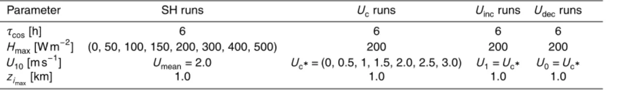
In Fig. 3, we show the modeled and observed shear production for the afternoon of 20 June. It is clear that even though the model has roughly the correct order of magnitude at 2.23 and 3.23 m, the modeled shear production term is decaying 20

too quickly with height to a value of near zero at about 60 m. The measured shear production may instead indicate that in the middle of the boundary layer, some mixed layer shear production takes place, which is not accounted for in this model driven by only surface measurements and boundary layer depthz_i. The wind gradient expression we have used is also only meant to be used in the surface layer, and our measurements 25

(16)

ACPD

15, 29807–29869, 2015

E. Nilsson et al.

Title Page

Tables Figures

◭ ◮

Back Close

Full Screen / Esc

Discussion

P

a

per

|

Discussion

P

a

per

|

Discussion

P

a

per

|

Discussion

P

a

per

|

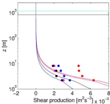
3.3.3 Height dependence of transport of TKE

Figure 4 shows the modeled and observed transport term of the TKE budget. The modeled transport term consists of both a transport due to buoyancy produced TKE and shear produced TKE. Such an approach may of course be criticized as turbulence in reality cannot be separated in such a way, but we are nevertheless not the first 5

(Mangia et al., 2000) to suggest such an approach when attempting to simplify the situation for a simple model. Based on studying vertical profiles of transport in sheared convective large-eddy simulations, we adapt a very idealized transport termT which consists in one partTbmore directly related to the buoyant production and one transport Ts that is related to the shear production term. At each height they are related as: 10

T=Tb+Ts. (9)

The termTbis given by a linear increase with height with slopek1for heightszup to

the boundary layer depthz_i as:

Tb(z)=Tb0+k1z. (10)

At the boundary layer heightz_i, the term reaches a maximum valueT_b_max and above 15

the boundary layer depth a symmetric−k1slope is assumed so that theTbis given by:

Tb(z)=Tbmax−k1(z−zi). (11)

This also determines the height of no turbulencezi0 as the height abovezi where

Tb(z) becomes 0. The surface value Tb₀ needs to be specified and it is determined

by a fractionT_f of the total transport to the total near surface production and the time 20

dependent surface buoyant production of TKE as

(17)

ACPD

15, 29807–29869, 2015

E. Nilsson et al.

Title Page

Tables Figures

◭ ◮

Back Close

Full Screen / Esc

Discussion

P

a

per

|

Discussion

P

a

per

|

Discussion

P

a

per

|

Discussion

P

a

per

|

We shall soon determineTf from measurements, but first to solve Eqs. (10) and (11)

we also need the slopek1which is given by:

k1=

Tb_max−Tb₀

z_i−0 . (13)

We solve forT_b

max by requiring that the transport term Tb integrates to zero over the

depth of the turbulent boundary layer. That is, from the surface to zi0. Given the 5

transport fractionTf, the termTbcan now be solved for, but this only makes up one part

of the total transport term in the model. In accordance with Eq. (9), we will first describe the transport related to shear productionTs. This term is given by the expression:

Ts(z,t)=−(Tf−p)S(z,t)(1−z/zi0). (14)

S(z,t) is the height and time dependent shear production, Tf is the near surface 10

transport fraction andpis a small positive free parameter that is determined such that the transport termTsintegrates to zero over the depth of the turbulent boundary layer.

This produces a transport profile with a negative layer near the surface transporting some of the near-surface shear generated TKE to the upper levels and a positive area above, that spreads the transport over the turbulent boundary layer. It also implies 15

that the factorpalters the near surface transport fraction value, but usually only a few percent.

Finally, the transport fractionTf, defined as the ratio of (minus) the total near surface

transport and the sum of near surface shear and buoyancy production, is given as az/L dependent function, based on our TKE budget analysis in Part 1 where we determined 20

φ_T,φbandφm, such that:

Tf(z/L)= −φ_T φb+φm

=1+ 0.54z/L−0.45

0.7(1−15z/L)−1/4₋_z/L. (15)

(18)

ACPD

15, 29807–29869, 2015

E. Nilsson et al.

Title Page

Tables Figures

◭ ◮

Back Close

Full Screen / Esc

Discussion

P

a

per

|

Discussion

P

a

per

|

Discussion

P

a

per

|

Discussion

P

a

per

|

of the stability parameterz/L. It is a good match to data for the morning period (blue circles and bin-averaged data with error bars) except possibly very close to neutral where the error bars are much larger mainly because of a specific time period in the morning of 25 June with indication of transport to the near-surface layers either from above or through a horizontal advection of TKE. Also, in comparison to the afternoon 5

data, the expression is a good match very near neutral, but it potentially overestimates transport over the range of−z/Lbetween about 0.5 to 7. It is, however, within the one standard deviation error bars. A different z/Lexpression, which may fit the afternoon data better, would still not be general as it would degrade the performance during the morning period. Future work should be aimed at understanding if the observed 10

difference between the build-up and the decay phases of turbulence are linked to some other non-dimensional parameter combination. As a first approximation, we apply the presented relationship at the first grid point 1 m above the surface in our model. In the case of the forest, the relationship is instead applied at the first grid point above displacement heightd.

15

The resulting profile of total transport shown in Fig.4 compare qualitatively quite well to the modeled transport term in Lenschow (1974) with a negative layer in the lower boundary layer and positive layer above. A linear profile shape in the mixed layer and a stronger curvature near the surface due to the e_ffect of shear production is also present in both models (Figs. A1 and A2). The exact value of this term on 20

specific heights differ, however, between these two models due to our inclusion of TKE budget terms also above the boundary layer depth zi and because of our specified

near-surface transport fraction. In near-neutral conditions the model from Lenschow (1974) obtain negligible transport in comparison to shear production and dissipation terms (see Fig. A2) whereas we retain more transport also in these conditions (with 25

Tf≈0.36). For very convective conditions we obtained Tf=0.46 whereas Lenschow

(1974) has a transport fractionTf≈0.57. This is of course an uncertain parameter that

(19)

ACPD

15, 29807–29869, 2015

E. Nilsson et al.

Title Page

Tables Figures

◭ ◮

Back Close

Full Screen / Esc

Discussion

P

a

per

|

Discussion

P

a

per

|

Discussion

P

a

per

|

Discussion

P

a

per

|

3.3.4 Height dependence of the dissipation term

The dissipation rate of TKE is calculated in the model using the TKE length scale parametrization presented in Part 1:

D=−E 3/2

l_ǫ =−E 3/2

2.2

zi +

0.006 z

. (16)

The modeled profiles of dissipation for the afternoon of 20 June are shown in Fig. 6 5

as colored lines and shown with both the near-surface dissipation as dots, UHF wind profiler estimates from 175 m as lines with circles and estimates from aircraft as crosses at two height intervals of 75 m for 14:30 and 17:30 UTC. Near the surface, it is clear that the modeled dissipation decays more rapidly with height than it should because of too rapidly decaying in the shear production term, leaving to little shear 10

produced TKE (=E) at 8 m. The modeled dissipation in the boundary layer compares well to the aircraft estimates of dissipation and in order of magnitude to the UHF profiler estimates. However, the UHF profiler estimates shows a maximum at some height around 500–600 m, which the model and aircraft measurements do not show. It is not easily determined if this often seen feature in UHF profiler estimates is realistic. Large-15

eddy simulations for this day did not show a pronounced maxima in dissipation rate. The only way our simple parametrization could produce such a maxima in dissipation rate is if the TKE itself has a maximum at these heights. Vertical wind variance is well known to have a maximum at some height around 0.3–0.4z_i, whereas LES often produce a maximum of TKE closer to the surface (below 100 m). Also, this simple model 20

predicts such a feature on several of the more convective days at around 40–50 m but fails to do so on 20 June as we will see in the next subsection. Qualitatively the vertical profile of dissipation is similar in our model compared to the model from Lenschow (1974), illustrated in Figs. A1 and A2, with higher dissipation closer to the ground but with some important differences with increasing height. The dissipation approaches 25

(20)

ACPD

15, 29807–29869, 2015

E. Nilsson et al.

Title Page

Tables Figures

◭ ◮

Back Close

Full Screen / Esc

Discussion

P

a

per

|

Discussion

P

a

per

|

Discussion

P

a

per

|

Discussion

P

a

per

|

it responds to the decreasing turbulence levels with increasing height. The exact level of dissipation in the two models close to the surface is also different under different stratification, mainly due to our different approaches to model vertical transport of TKE.

3.3.5 Height and time dependence of TKE

The evolution of TKE is determined by a finite difference (forward in time) calculation 5

with 1 s time step and 1 m vertical resolution from the other budget terms using the TKE budget equation.

E(z,tn+1)−E(z,tn)

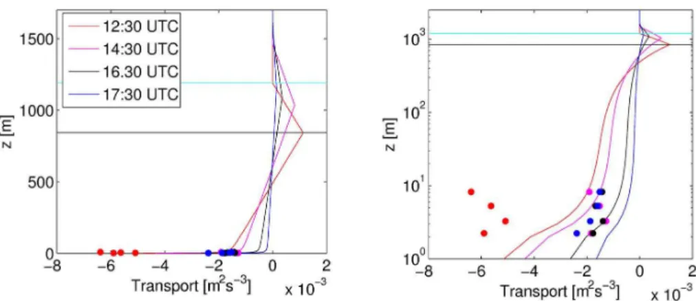
∆t =S(z,tn)+B(z,tn)+T(z,tn)+D(z,tn) (17) The resulting vertical profiles of TKE are shown in Fig. 7 for the afternoon of 20 June. In this figure, TKE at the small tower (2.23–8.22 m) was averaged and a standard 10

deviation was calculated for each hour centered around 12:30, 14:30, 16:30 and 17:30 UTC. The result is shown with a vertical error bar indicating the minimum and maximum of the data. The same procedure was applied for the 60 m tower data, which consistently showed lower TKE levels compared to the near surface TKE. The procedure was also applied to limited 3-D-sonic anemometer data from a sensor 15

suspended from a tethered balloon (see Lothon et al., 2014, for details). Data were available at ≈70 m and 520 m above ground at 12:30 and 17:30 UTC. At 14:30 and 16:30 UTC, the tower data has been slightly vertically displaced to better show the error bars without overlapping too much.

It is clear that the model produces TKE of the right order of magnitude and predicts 20

the general reduction of TKE with height from the smaller tower to the 60 m tower. The decay of TKE in time may, however, be somewhat to rapid in comparison to measurements, as indicated by the low TKE levels at 16:30 and 17:30 UTC. However, the individual levels on the towers (2.23 and 61.4 m) will be shown in time series plots in the next section which have quite reasonable levels of TKE for 20 June considering 25

(21)

ACPD

15, 29807–29869, 2015

E. Nilsson et al.

Title Page

Tables Figures

◭ ◮

Back Close

Full Screen / Esc

Discussion

P

a

per

|

Discussion

P

a

per

|

Discussion

P

a

per

|

Discussion

P

a

per

|

The model only predicts an increase of TKE from the first model level to the second, due to the prescribed reduced shear production at the first grid point compared to the others. Otherwise, the model shows a decrease in TKE with height, which is not necessarily true at all height ranges. The measurements often show a small increase in TKE from 2.23 to 8.22 m (as is clear from Table B3 in Part 1), but consistently lower 5

TKE levels at the 60 m tower imply a maximum of TKE somewhere close to the surface at a height on the order of tens of meters. As mentioned above, this simple model is capable of predicting a maximum of TKE near the surface at around 40–50 m for some of the more convective days of the field campaign. Then the model also often overestimates the TKE level at the 60 m tower. This could indicate that the maximum 10

of TKE should be placed even lower than 40 m.

3.3.6 Specification of initial neutral morning conditions

The TKE budget equation is used to solve for the evolution of TKE from neutral morning conditions until the end of the afternoon. At the beginning of the simulation, for simplicity, we therefore assume the buoyant production termB(z) to be zero at all 15

heights. The shear production termS(z) is calculated as before. The transport term is in this case only specified from the transport fraction and the shear term as−S(z)T_f to avoid an uncompensated positive layer in the upper part of the boundary layer.

Our treatment of initial conditions for dissipationD(z) and turbulence kinetic energy E(z) also differs from other time steps since there is no history of the flow to take into 20

consideration at the first time step. Here, we first assume that the initial TKE tendency is negligible (such that ∂E_∂t =0) and then solve forD(z) based on the shear production and transport term, henceD(z)=−(S(z)+T(z)). Then, we use this initial dissipation

and estimate an initial TKE profile fromE(z)=−ziD(z)

2 2/3

such that the dissipation in the following time step will not obtain a large sudden jump when using the profileE(z) 25

(22)

ACPD

15, 29807–29869, 2015

E. Nilsson et al.

Title Page

Tables Figures

◭ ◮

Back Close

Full Screen / Esc

Discussion

P

a

per

|

Discussion

P

a

per

|

Discussion

P

a

per

|

Discussion

P

a

per

|

model tests showed small differences in results for the evolution of modeled TKE at midday and afternoon.

4 Evaluation of near surface TKE and budget terms: 9 IOP days

In this section, we compare the simple model to measurements for 9 IOP days studied in Part 1. The first objective is to investigate the simple model’s ability to predict 5

a reasonable near surface TKE and TKE budget evolution for the diverse set of conditions that occurred on these 9 days despite its deficiencies. The second aim is to discuss why the model produces unreasonable results. This indicates potential focus areas for future model improvement.

The upper row of Fig. 8 shows the model’s stability corrected friction velocity u∗ 10

as black lines and observations at 3.23 m as red lines with dots. It is clear that our approach gives reasonable estimates ofu_∗on many occasions, but also it misses some low and especially high values that occur for periods of 1 or 2 h. Further, the modeled friction velocity, based on mainly the mean wind speed, does not always reflect this observed variability and produces a more smooth evolution ofu_∗ for each day.

15

The middle row of Fig. 8 shows the measured wind speed gradient based on 10 min values as thin colored lines with dots and the modeled wind speed gradient as thicker colored lines. In this case, it is clear that wind gradients shift rapidly and the model captures some of the low frequency variability of the observations. This is, however, not always the case (see e.g., 27 June as well as 2 and 5 July).

20

The observed hourly shear production is shown in the lower row of Fig. 8 with colored dots. The model (thick lines) does capture some of the day to day variability, but the smooth model results do not capture all of the individual hourly variability seen in the measurements. Furthermore, shear production tends to be underestimated at times with higher shear production such as on 25 and 26 June. This underestimation is more 25

(23)

ACPD

15, 29807–29869, 2015

E. Nilsson et al.

Title Page

Tables Figures

◭ ◮

Back Close

Full Screen / Esc

Discussion

P

a

per

|

Discussion

P

a

per

|

Discussion

P

a

per

|

Discussion

P

a

per

|

afternoon of 27 June and to some extent, on 20 June and in the middle of the day on 1 July.

The observed and modeled near surface buoyant production is shown in the upper row of Fig. 9 and is in general a good (albeit smoothed) representation of the measurements. On 20 June at 12:30 UTC, the model underestimates the measured 5

buoyancy production at 5.27 and 8.22 m as was already noted in Fig. 3. On 30 June, which had variable cloud cover, similar errors are also seen, but otherwise in most cases the differences between model and measurements are smaller for this more directly forced budget term.

The middle row of Fig. 9 shows the modeled and observed transport, which show 10

significantly larger scatter in observed values compared to the buoyant production and larger individual discrepancies between model and measurements. Particularly on days with more wind, the scatter is larger such as on 20, 25–27 June. As discussed, it is challenging for the model to capture the shear production well on an hourly basis and also the modeled transport has a smoother evolution in time than the observations. 15

The lower row shows the observed and modeled dissipation. The model captures much of the day to day as well as hourly variability, but at times of strong shear production, it underestimates at the 8.22 m level. This is observed on 25, 26 and the afternoon of 27 June as well as in the middle of the day on 1 July. The model also overestimates dissipation somewhat on 2 July and during the morning period of 5 July 20

until around 12:00 UTC.

All these observed errors in the modeled TKE budget terms, which may at times be considered quite small, can lead to problems in the prediction of the TKE as any systematic errors can cause an accumulated effect for the TKE prediction. We therefore find the modeled results of TKE at the 2.23 m level and 61.4 m level presented in 25

(24)

ACPD

15, 29807–29869, 2015

E. Nilsson et al.

Title Page

Tables Figures

◭ ◮

Back Close

Full Screen / Esc

Discussion

P

a

per

|

Discussion

P

a

per

|

Discussion

P

a

per

|

Discussion

P

a

per

|

For the 2.23 m level, shown in the lower row of Fig. 10, the model underestimates the TKE on 8 out of 10 days at the beginning of the simulation up until around 08:00 or 09:00 UTC (at least). This is probably mostly related to uncertainty in the way we define initial profiles of TKE for neutral morning conditions. The level of TKE at 2 m during midday is relatively well-captured on many of the days but too low on 2 and 5 5

July. On 2 July and the morning of 5 July this could be due to a slight overestimation of near surface dissipation. On 5 July there are also a few hours of an observed positive transport term at some heights (and small at other heights), implying a potential import of near surface TKE, which if it did occur cannot be captured by the simple model. This was also observed very temporarily on 27 and 30 June, which as discussed in Part 1, 10

could be related to variable cloud cover and/or uncertainty in dissipation estimates. With this one dimensional model, it is difficult to draw conclusions regarding the import of TKE from above or by horizontal advection. On the morning of 25 June, however, there are several hours with observed positive values of the transport term at all measurement heights and this may have additionally contributed to an underestimation 15

of near surface TKE in the morning of this day.

At 61.4 m, the TKE level is underestimated on 25 and 26 June and at the end of the afternoon on 27 June. It is likely a consequence of too rapidly decaying shear production with height. The model also tends to overestimate TKE on some days with higher buoyancy production (e.g. 24, 30 June, 1 and 2 July). It is unclear, however, 20

to what extent the observed differences at 60 m should be related to issues with the model or related to differences in fluxes and wind that occur at different surfaces in the landscape surrounding the 60 m tower. It may of course be that the observed flux and wind at the Divergence Site is not always representative for a height of 60 m. A flux footprint analysis (Hartogensis, 2015) for the 60 m tower indicates that grass and moor 25

(25)

ACPD

15, 29807–29869, 2015

E. Nilsson et al.

Title Page

Tables Figures

◭ ◮

Back Close

Full Screen / Esc

Discussion

P

a

per

|

Discussion

P

a

per

|

Discussion

P

a

per

|

Discussion

P

a

per

|

North-East the flux is especially dominated by grass and moor conditions (Hartogensis, 2015), but this changes when the wind comes from East. Interestingly we observe that the model underestimates the TKE especially when the wind in the lower CBL and near the surface is from East, rather than typically from North or North-East for the rest of the time. The easterly flows happen on 25 and 26 June, in the late afternoon of 27 June 5

and in the morning of 5 July (see wind direction close to the surface in Part 1, Fig. 3). All these periods correspond to an underestimated TKE in the model at 61.4 m. This could be linked with the presence of a band of forest to the East and the Lannemezan village behind, and that either the flux or the shear production that we use do not represent their effect. It could also be due to advected TKE from the East. These effects related to 10

heterogeneity in the landscape in combination with shifting wind direction also causes the reconstructed flux (at the 60 m tower) to have a variable contribution from different surface land covers both on a daily and hourly basis. A flux footprint analysis may, however, not be directly translated to apply for a variable such as TKE. Therefore we mainly conclude that the model performs reasonably well at 2.23 m and less well, but 15

still with the right order of magnitude for TKE at 61.4 m.

5 Sensitivity test of surface boundary conditions: influence on boundary layer

dissipation rate and the formation of a pre-residual layer

As an exploration into the sensitivity of model results to different observed fluxes and winds over different surface types, we show in Fig. 11 modeled dissipation rate for 20

30 June from five simulations over corn, moor, forest, wheat and grass with available measurements. Also shown are model results for the Divergence site and using a 2 by 2 km area-averaged flux, as well as the observed dissipation rate from a UHF wind profiler. On this day, there was no distinguishable bias between dissipation rates from the UHF profiler and aircraft measurements (not shown here) and therefore 25

(26)

ACPD

15, 29807–29869, 2015

E. Nilsson et al.

Title Page

Tables Figures

◭ ◮

Back Close

Full Screen / Esc

Discussion

P

a

per

|

Discussion

P

a

per

|

Discussion

P

a

per

|

Discussion

P

a

per

|

The Divergence Site tower measurements show very similar low fluxes as observed over grass and moor, and for this day, also corn. This is in contrast to the higher observed fluxes over forest and wheat. The surface flux over the grass, moor, corn and Divergence sites yielded the most similar levels of dissipation rate compared to the observations on this day, whereas other surface types lead to higher levels 5

of dissipation rate. Based on energy balance modeling, fluxes of urban and bare soil land covers were also determined to be high, corresponding roughly to the forest level (Hartogensis, 2015). Especially, we believe that the urban land cover used likely overestimate the real flux from the villages considered here, which have much vegetation between the houses. Therefore, using area averaged fluxes over 10

a 2 km×2 km or 10 km×10 km area of the surroundings lead to higher estimates of boundary layer TKE and dissipation rates compared to using the Divergence Site observations.

We note that the model may overestimate boundary layer dissipation somewhat for 30 June and turbulence may not be as capped in the model as indicated from 15

UHF profiler. The simple model presented here lacks elevated wind shear in the entrainment zone, which may lead to an underestimation of dissipation rate and TKE in the upper parts of the boundary layer. Elevated shear may, however, also affect the entrainment process and the entrainment parameter which here has been simply taken as a constant value of−0.15 based on a study for 20 June. Model tests changing this 20

value to −0.3 showed reduced levels of TKE and dissipation rate in the upper parts of the boundary layer, but with otherwise similar results and only a small impact in the lower part of the boundary layer.

An apparently important result from this study is that the modeled decay of dissipation rate and TKE occurs first at the upper part of the boundary layer during the 25

(27)

ACPD

15, 29807–29869, 2015

E. Nilsson et al.

Title Page

Tables Figures

◭ ◮

Back Close

Full Screen / Esc

Discussion

P

a

per

|

Discussion

P

a

per

|

Discussion

P

a

per

|

Discussion

P

a

per

|

of TKE dissipation rates from top to bottom (although not systematically). This was also used as a way to define a top of the turbulent boundary layer in the afternoon transition in numerical weather prediction models (Couvreux et al., 2015). In Fig. 11 the white line shown is an iso-line for TKE (corresponding to 0.3 m2s−2), which is of course an arbitrarily chosen value, but it indicates low turbulence levels. It is instructive 5

from a conceptual point of view to consider these conditions with low turbulence levels during the afternoon transition as a pre-residual layer. It forms when the boundary layer turbulence adjusts to the weaker buoyancy flux forcing from the surface. It is capped by the mixed-layer inversion and does not reach the surface except possibly very near neutral stratification at the end of the afternoon or the beginning of the 10

evening transition. It is useful to introduce this concept of a pre-residual layer as we consider that it is an important part of explaining the onset turbulence conditions for the nocturnal residual layer.

The residual layer is defined as the statically neutral layer, characterized by weak sporadic turbulence, that lies above the stable boundary layer and below the capping 15

inversion, separating the boundary layer flow from the free atmosphere. By definition, it begins to develop only after the surface begins to stably stratify. Therefore, it is useful to also name the region of weak turbulence that exists during unstable conditions preceding the residual layer as the pre-residual layer. It is within these continuously weakening afternoon turbulence conditions that many things characterizing the 20

turbulence are changing, such as the shape of spectra of vertical wind velocity and integral length scales (Darbieu et al., 2015). Darbieu et al. (2015) showed with LES and measurements that change occurs first in the upper part of the boundary layer during the later stages of the afternoon transition, and the higher within the ABL the stronger the spectra changes. These observations may hence be considered to have 25

(28)

ACPD

15, 29807–29869, 2015

E. Nilsson et al.

Title Page

Tables Figures

◭ ◮

Back Close

Full Screen / Esc

Discussion

P

a

per

|

Discussion

P

a

per

|

Discussion

P

a

per

|

Discussion

P

a

per

|

6 Parameter exploration for near-surface TKE

In this section, we first discuss modeled near-surface TKE for the afternoon based upon complementary idealized numerical simulations. Secondly, we compare our numerical model results to a simplified analytical expression assuming quasi-stationary turbulence. Finally, we illustrate and discuss the added value of our modeling efforts 5

taking into account variations in wind oru_∗ compared to only taking into account ofw_∗ as a scaling variable for TKE.

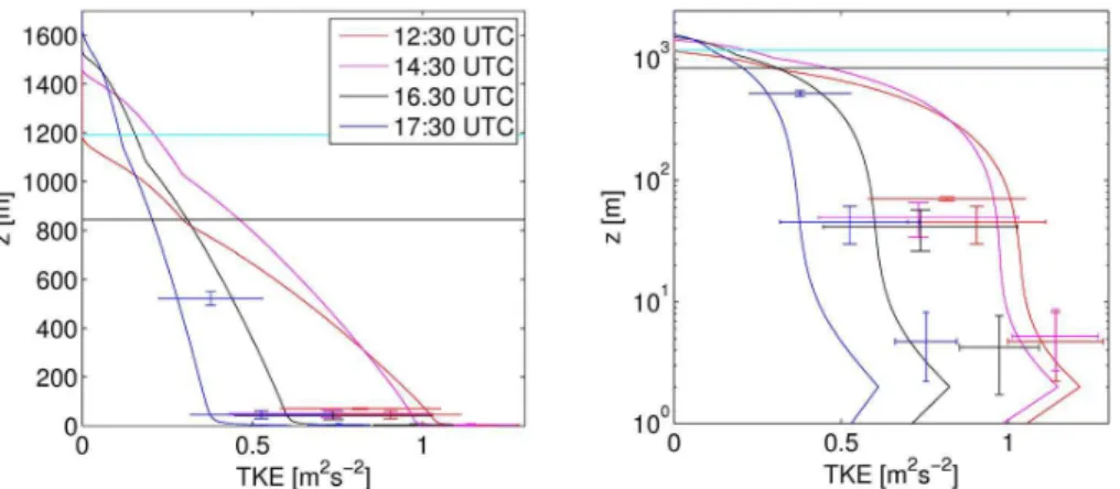
The sensible heat flux used in these model runs are provided by a cosine function as in Sorbjan (1997) and several other earlier studies:

Hcos(t′)=Hmaxcos

2t′ πτcos

. (18)

10

Here, Hmax defines the maximum sensible heat flux in midday and the decay time

scaleτcosdefines the length of the period with positive sensible heat flux (half of which

covers the afternoon period). For simplicity, we chose a zero latent heat flux in these idealized simulations.

For boundary layer depth, we specify a very simple sine function increase ofz_i from 15

a neutral morning valuez_i

min to a midday valuezimax by

zi(t′)=zi_min+(zi_max−zi_min) sin

2t′ πτcos

, (19)

which is then kept constant for the afternoon.

The complementary idealized numerical simulations have been performed by systematically varying a studied parameter while keeping all the other variables 20