When imagining future wealth influences risky decision making
Adam Eric Greenberg
∗Abstract
The body of literature on the relationship between risk aversion and wealth is extensive. However, little attention has been given to examining how future realizations of wealth might affect (current) risk decisions. Using paired lottery choice experiments and exposing subjects experimentally to imagined future wealth frames, I find that individuals are more risk-seeking if they are asked to imagine that they will be wealthy in the future. Yet I find that individuals are not significantly more risk-averse if they are asked to imagine that they will be poor in the future. I discuss theoretical and policy implications of these findings, including why savings rates are so low in the United States.
Keywords: risky decision making, framing, wealth, savings, expected utility.
1
Introduction
Understanding the effect of future wealth on risk aversion is essential for uncovering the puzzle of why household savings is low in the United States. In particular, there are compelling reasons to believe that many choices are mo-tivated, in part, by how we imagine our future states of wealth. Individuals constantly struggle between “risky” and “safe” options—whether to become a rock star or a music teacher, be an entrepreneur or work for a com-pany, etc.—that are ultimately chosen based on upside or downside potential. But I know of no research that exam-ines the relationship between imagined future wealth and risky decision making.
The relationship between wealth and risk aversion is well-documented in the economics literature (Kihlstrom et al., 1981; Brunnermeier & Nagel, 2008; Sousa, 2010; Paravisini et al., 2011). Yet pioneers of the theory of the utility of wealth did not reach a consensus about the direction of this relationship.1 Expected-utility
the-ory (EUT) remains the dominant framework for examing the relationship between wealth and risk. EUT predicts that individuals maximize their expected utility based on probabilities and outcome utilities of possible levels of
A version of this paper constituted my senior thesis at Vassar Col-lege. I am indebted to Sean Masaki Flynn for his guidance and support. I am grateful to two anonymous referees as well as Jonathan Baron and Jean-Robert Tyran for insightful comments. I also thank Ben Brad-shaw and Vincent Leah-Martin for excellent research assistance. This research was supported by the Academic Support and Enrichment Fund at Vassar College.
Copyright: © 2013. The authors license this article under the terms of the Creative Commons Attribution 3.0 License.
∗University of California, San Diego, Department of Economics,
9500 Gilman Drive, La Jolla, CA 92093; aegreenb@ucsd.edu
1Friedman and Savage (1948) argued that the curvature of the
util-ity function predicts a lower propensutil-ity for risk in wealthy individuals and a greater taste for risky decisions in less wealthy individuals, while Markowitz (1952) argued the opposite relationship.
wealth. But extensive research (e.g., Kahneman & Tver-sky, 1979; Rabin, 2000; Rabin & Thaler, 2001) has chal-lenged the sufficiency of EUT as a descriptive account. Inquiries about how future reference point realizations could affect (current) economic decisions have not been investigated. In particular, how does imagining a future wealth scenario change our decisions today? This type of question has several economic applications; its impli-cations for savings behavior, in particular, are discussed here.
This paper studies behavior in paired lottery choice experiments to experimentally test whether hypotheti-cal future realizations of wealth alter individuals’ current risk decisions. In particular, I am interested in whether changes in hypothetical wealth frames affect risk aver-sion. My hypotheses are derived from EUT with decreas-ing relative risk aversion. I hypothesize that (H1) those who imagine they will be wealthy will take more risks because they are prompted to think that they can afford to take more gambles and (H2) those who imagine they will be poor will take fewer gambles since they believe they cannot afford to take risks. EUT with decreasing rela-tive risk aversion would predict that individuals respond to an exogenous increase in wealth by taking more risks and respond to a decrease by taking fewer. I find that those who are asked to imagine themselves as wealthy in the future make significantly riskier decisions today. Yet those who are asked to imagine themselves as poor in the future are not significantly more risk-averse in their cur-rent decisions.
2
Previous work
The existing research on how framing affects choice is extensive (beginning with Tversky & Kahneman, 1981,
and Hershey et al., 1982). It is important to note, as well, that framing has real effects on economic behavior. Con-sistent with prospect theory, researchers have found that gain and loss frames alter choice decisions, even if the underlying decisions are the same. Epley and Gneezy (2007) argued that the framing of financial windfalls can change how people spend their income. In particular, in-come that is perceived as a positive departure from indi-viduals’ reference points (e.g., bonus) is spent more eas-ily than that which is perceived as undoing a negative de-parture (e.g., refund).
In addition, the outcomes of prior events have been shown to affect identical decisions. Coval and Shumway (2005) found that investor losses in the morning often lead to risky behavior in afternoon trading. In this case, while investment decisions should be based on future re-turns, they are also based on whether the investor is a winner or a loser at the time of the decision.
While economic theory has predictions for how expec-tations about the future affect current decisions, empirical and experimental tests are sparse. One such study exam-ining the link between expected future income and risk decisions using survey data found that households that are more likely to face uncertainty about future income or about to become liquidity constrained are more risk-averse (Guiso & Paiella, 2008). In another study, Carroll (1994) reports that consumption decisions are unaffected by expected changes in income, which is consistent with consumption smoothing. Binswanger (1980) found that wealth reduces risk aversion, but only slightly (and not significantly). But this study, in particular, did not ex-amine future wealth, and its sample comprised unskilled laborers in rural India.
The present study is apparently the first to experimen-tally test the relationship between imagined future wealth and (current) risk decisions. I examine the effect of fu-ture wealth frames (wealthy and poor) on hypothetical risky decisions involving money. These types of frames are common in the psychology literature as experimental tools (Garry et al., 1996; Anderson, 1983; Carroll, 1978). In one recent example, Beegle et al. (2012) asked house-holds in Tajikistan to rank their own economic statuses against theoretical vignettes of other households to see whether they had a frame-of-reference bias with respect to their own welfare. They found that households had di-verse scales for assessing their levels of welfare, and that the bias is actually quite small. Here I use similar types of vignettes.
3
Experimental design
Registered undergraduate students at Vassar College were recruited primarily through informal
announce-ments such as Facebook, word of mouth, and email. They were told that the experiment consisted of two sessions (“Session I” and “Session II”), each taking 20–25 min-utes. They were also informed that the two sessions would be a week apart and would be completed online. Before each session, directions for logging into the ex-periment were sent to campus email addresses provided by the subjects.
Subjects were randomly assigned to one of three groups—two treatment groups and a control group. The first treatment group was the “Wealthy then Poor” group. Subjects assigned to this treatment were given a “Wealthy” frame (Appendix A) in Session I in which they were asked to imagine that they became wealthy in the future. After subjects read this frame, they were in-structed: “Please put yourself in the position of the per-son described in this frame and proceed to the decisions.” The subjects then completed a series of 10 paired lottery choice decisions first utilized by Holt and Laury (2002) to yield a measure of their risk preferences.
A week later, these subjects were given a “Poor” frame (Appendix A) in Session II in which they were asked to imagine that they became poor in the future. After read-ing the Poor frame, they were given the same instructions they received in Session I and completed the same Holt and Laury (2002) risk preference assessment.
Subjects assigned to the second treatment group, “Poor then Wealthy”, completed the same risk assessment ques-tions, but were given the frames in the opposite order. Fi-nally, the control group (“Control”) subjects completed the lottery choice questions, but were given neither the Wealthy nor the Poor frames in either session.2 For all
three groups, Session II lottery decisions were followed by a brief demographic questionnaire.
For each of the ten pairs of risk-assessment questions in the Holt and Laury (2002) setup (Appendix B), sub-jects are asked to choose between a “safe” bet (which we call “Option A”) and a “risky” bet (“Option B”). In the safe bet, there is a relatively small differential between the higher payoff amount and the lower payoff amount. In the risky bet, the differential between the payouts is rather large. The respective nominal payouts for Option A and Option B do not change between the ten decisions.
2In the place of frames, subjects in the Control group saw a blank
What does change, however, is the relative probability of obtaining the higher payoff amount. Instructions for the decision task resembled those given in Holt and Laury (2002).
Note that by having both Sessions I and II, we are ran-domizing order of frames within-subjects. However, if we examine only Session I, we have a between-subjects analysis. Results from both analyses are described in the next section.
Subjects included 190 undergraduate students (from a variety of majors), with 65 in each treatment group and 60 in the Control group.3The median time spent between
Sessions I and II was 9 days, while the range was 8 to 13 days. Each subject was told that one of her 10 decisions made in each session would be selected at random and that her gamble (fixed by her choice of either Option A or Option B) in the selected decision would be performed to determine her payout. Potential payouts had to be small enough so as to not encourage “erratic” behavior.4 For
this reason, the payoffs for all treatments were equal to the lowest payoff in the experiments conducted by Holt and Laury (2002) multiplied by 4.5
Subjects were paid the average of theirsession payoffs
from Session I and Session II. Each session payoff was determined by performing one gamble randomly chosen from the list of ten decisions in the elicitation task (Ap-pendix B). For instance, suppose I chose Option B for decision 4 in this particular session, and the computer rolls a 10. My session payoff is $0.40. The same cal-culation would be done for the other session, and the two session payoffs would be averaged to compute my total payoff. Thus, while payoffs were based on gambles, sub-jects knew for certain that each of the two sessions would carry equal weight in their total payoffs. To avoid poten-tial time-preference confounds6, subjects received their
payoffs by check in their campus mailboxes about a week after Session II was completed. The mean payoff was $4.42, and there were no show-up fees.
3There were 11 other subjects that did not complete both sessions.
Because we were unable to observe their behavior across frames (or across Control treatments), these subjects are excluded from the analy-sis.
4Holt and Laury (2002) tested whether people are more risk-averse
when payoff treatments are scaled up and whether behavior varies be-tween hypothetical and real monetary payoffs. In one of their high-payoff treatments, the safe option provides either $144 or $180 while the risky option provides either $346.50 or $9. One-third of the subjects chose the safe option until the final decision in which the higher payoff was a certainty. In the low-payoff treatment, however, the majority of subjects chose 4 to 6 safe choices (as opposed to 9).
5Multiplying Holt and Laury’s (2002) numbers by 4 was somewhat
arbitrary. However, it was important that the payoffs be non-negligible for undergraduates, but not large enough to generate “erratic” results.
6For example, see Andreoni and Sprenger (2012).
4
Results
The only difference between the “Wealthy then Poor” (N = 65) and the “Poor then Wealthy” (N = 65) treatments is the order in which subjects observed the future wealth frames. The main reason for including these two treatments was to test for order effects. Us-ing Mann-WhitneyU-tests to compare the results from the two Wealthy frames and the two Poor frames and a Wilcoxon test to compare the two sessions of the Control group (N = 60), we find no statistically significant dif-ferences, indicating similar distributions across sessions. Thus we fail to reject the null hypothesis that there were order effects in the experimental treatments. In the ab-sence of order effects, we aggregate subjects within each frame (or lack thereof) rather than within each treatment. Holt and Laury’s (2002) risk aversion instrument yields implicit risk preferences. Under constant relative risk aversion (CRRA), a risk-neutral subject, for exam-ple, will choose Option A (safe bet) for the first four de-cisions, then Option B (risky bet) for the latter six deci-sions. Subjects who are risk-averse will choose Option A for more than four decisions before switching to Option B, while those who are risk-seeking will choose Option A for fewer than four choices before switching to Op-tion B.7That said, we expect subjects to switch only once
from Option A to Option B.
The vast majority of subjects (178 out of 190) chose Option A for some number of decisions before switching over to Option B, without ever switching again. In 21 cases, subjects chose Option B for every decision.8 Only
16 subjects switched between Option A and Option B more than one time.9In the tenth decision—which offers
a choice between a sure payoff of $8.00 and a sure pay-off of $15.40—only 2 subjects in the entire experiment chose Option A, the lower payoff, most likely indicating that these 2 subjects might not have fully understood the instructions.10
7The relatively arbitrary choice of this “switch” point has been
shown to present spurious correlations in experiments with noisy decision-making biases. Using similar multiple price lists, Andersson et al. (2013) found that placing the switch point at the third decision pro-duces a negative correlation between risk aversion and cognitive ability; whereas placing the switch point at the sixth decision produces the op-posite result. This is generated by heterogeneity in types correlated with risk aversion: types that are prone to make mistakes will appear more risk averse while those who are error-free will not. In the currrent pa-per, we are interested in how the frames change levels of risk aversion. While these decision-making biases may still be present, we do not need to worry since our effects of interest are randomly assigned.
817 of these cases occurred during the Wealthy frame; 3 during the
poor frame, and 1 during the control in Session I.
9Note that subjects who switched between Option A and Option B
more than once werenotexcluded. As a check for the robustness of results, we conducted the analysis with and without these subjects and found no significant differences. Thus we err on the side of keeping observations.
be-Table 1: Summary statistics: Number of safe choices. This table reports summary statistics for each treatment frame. All subjects completed risk assessment questions. Wealthy and Poor treatments represent risk assessments after being exposed to wealth treatment frames in which subjects were asked to imagine themselves as wealthy or poor, respectively. The Control group subjects were given no frame at all. Controlirefers to choices made by the Control group in Sessionifori∈ {1,2}.
Treatment Mean Median S.D. N
Frame: Wealthy 3.89 4 2.14 130 Frame: Poor 5.62 6 1.82 130 Control 1 (No Frame) 5.32 5 1.58 60 Control 2 (No Frame) 5.45 5 1.58 60
To measure subjects’ degrees of risk aversion, I ob-served the number of times the subject chooses Option A, the safe bet. Recall that payoffs are constructed such that a risk-neutral utility-maximizer under CRRA will se-lect Option A for the first four decisions and Option B for the latter six. CRRA coefficients can be inferred using the number of safe bets chosen by subjects. In particu-lar, if a subject chooses Option A four times, her CRRA coefficient,ρ, is approximately zero (the range could be
−0.15 < ρ <0.15). If the number of safe bets exceeds four, thenρ > 0; if the number is less than four, then
ρ <0.11 Since the purpose of this study is to determine
whether future wealth frames affect individuals’ degrees of risk aversion, I simply compare how many safe bets they make in the decision experiments under each future wealth frame.
Table 1 reports the number of safe choices (out of 10 possible choices) made by subjects within each frame. Subjects who were given the Wealthy frame make, on average, 3.89 (sessions pooled) safe bets, while those in the Control group make, on average, 5.32 (Session I) and 5.45 (Session II) safe bets. Mann-Whitney U-tests al-low us to reject the hypothesis that subjects who saw the Wealthy frame do not make fewer safe choices than those in the Control group (H1). The difference in safe bets made is, in fact, statistically significant in both Session I (p= 0.0010) and Session II (p <0.0001). Also, subjects who were given the Poor frame made, on average, 5.62 (sessions pooled) safe bets. However, Mann-WhitneyU -tests do not allow us to reject the hypothesis that subjects who saw the Poor frame do not make more safe choices
gan. Nevertheless it is possible that a couple subjects might still not have understood the instructions.
11For a more complete risk classification by the number of safe bets,
see Holt and Laury (2002).
Figure 1: Mean number of safe choices by frame.
3.5
4
4.5
5
5.5
6
Mean Number of Safe Choices
Wealthy Poor Control 1 Control 2 Frame
than those in the Control group (H2). The difference in this case is not significant in Session I (p= 0.31) or Ses-sion II (p= 0.18). Figure 1 represents the mean number of safe choices by frame with confidence intervals.
In the within-subjects comparison, behavior changes in the expected direction. The vast majority (83 out of 130) of subjects given the frames chooses more safe bets in the Poor frame than in the Wealthy frame, while rela-tively few (16 out of 130) subjects choose more safe bets in the Wealthy frame. A Wilcoxon signed-rank test finds that difference in behavior across the Wealthy and Poor frames is significant (z = −6.86,p < 0.0001). Inter-estingly, some (31 out of 130) subjects also appear to not change behavior across frames.
By analyzing differences in the number of safe choices made under the future wealth frames (i.e., the Wealthy and Poor frames) and the Control group, we are able to in-fer difin-ferences in risk propensities across these frames. In particular, we find that subjects given the Wealthy frame are significantly more risk-seeking than those given no frame (the Control), and that those given the Poor frame are only not quite significantly more risk-averse than those given no frame. Thus, subjects were significantly more risk-seeking when asked to imagine themselves as wealthy in the future, but not quite significantly more risk-averse when asked to imagine themselves as poor in the future. In other words, imagining oneself as wealthy in the future does, in fact, affect current risk aversion, while imagining oneself as poor in the future may not. Note as well that the between-subjects design alleviates concerns about experimenter demand effects.
These results are confirmed when comparing decisions made under future wealth frames with the Control group within each session.12 The results are robust even when
12The difference between the number of safe choices made under the
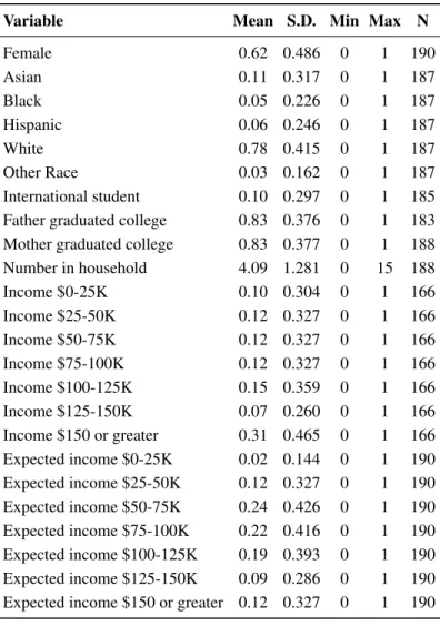
Table 2: Summary statistics: Demographics. This table reports summary statistics for demographic data reported by all subjects in the sample. All subjects completed self-reported questionnaires. Income brackets represent reported household income at time of experiment. Expected income brackets represent individual income expected ten years after college graduation.
Variable Mean S.D. Min Max N
Female 0.62 0.486 0 1 190
Asian 0.11 0.317 0 1 187
Black 0.05 0.226 0 1 187
Hispanic 0.06 0.246 0 1 187
White 0.78 0.415 0 1 187
Other Race 0.03 0.162 0 1 187 International student 0.10 0.297 0 1 185 Father graduated college 0.83 0.376 0 1 183 Mother graduated college 0.83 0.377 0 1 188 Number in household 4.09 1.281 0 15 188 Income $0-25K 0.10 0.304 0 1 166 Income $25-50K 0.12 0.327 0 1 166 Income $50-75K 0.12 0.327 0 1 166 Income $75-100K 0.12 0.327 0 1 166 Income $100-125K 0.15 0.359 0 1 166 Income $125-150K 0.07 0.260 0 1 166 Income $150 or greater 0.31 0.465 0 1 166 Expected income $0-25K 0.02 0.144 0 1 190 Expected income $25-50K 0.12 0.327 0 1 190 Expected income $50-75K 0.24 0.426 0 1 190 Expected income $75-100K 0.22 0.416 0 1 190 Expected income $100-125K 0.19 0.393 0 1 190 Expected income $125-150K 0.09 0.286 0 1 190 Expected income $150 or greater 0.12 0.327 0 1 190
we restrict the sample to subjects who never switched from Option A to Option B more than once.
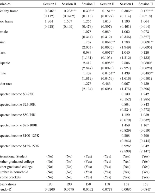
Table 2 reports the summary statistics of the demo-graphic variables collected after Session II. Table 3 re-ports the results from ordered logistic regressions of the number of safe choices made (a proxy for risk aversion) on sex, race, international student status, income, par-ents’ education levels, and the number of people in their households. Reported coefficients are proportional odds ratios and each observation is one subject in the experi-ment. The first two columns report results from the set of regressions in which subjects are pooled by each of the two sessions. This allows us to isolate the effect of each
between the number of safe choices made under the Poor frame and the Control is still not statistically significant when we restrict our attention to one session at a time.
wealth frame compared to the Control on the number of safe choices made by subjects. Here we find that the sub-jects who see the Wealthy frame can be expected to make significantly fewer safe choices than those in the Control group, all else equal. However, subjects who see the Poor frame do not make significantly more safe choices than those in the Control group.
Table 3: Ordered logistic regression of number of safe choices. The dependent variable is the number of safe choices (out of 10) in the risk assessment. Each set of two columns aggregates safe choices by frame (Wealthy, Poor, or Control in each session). Income brackets are dummy intercepts given by income ranges reported by subjects. Expected Income brackets are chosen by subjects to reflect expected income ten years after college graduation.
Variables Session I Session II Session I Session II Session I Session II
Wealthy frame 0.346∗∗ 0.233∗∗∗ 0.306∗∗ 0.181∗∗∗ 0.305∗∗ 0.177∗∗∗
(0.112) (0.0762) (0.115) (0.0727) (0.114) (0.0718)
Poor frame 1.364 1.567 1.255 1.610 1.190 1.664
(0.425) (0.499) (0.473) (0.597) (0.461) (0.614)
Female 1.078 0.969 1.062 0.973
(0.344) (0.312) (0.346) (0.327)
Asian 1.787 0.0646∗∗ 1.783 0.0691∗∗
(2.034) (0.0635) (1.949) (0.0695)
Black 0.983 0.0974∗ 1.040 0.120
(1.131) (0.105) (1.212) (0.132)
Hispanic 2.412 0.0985∗ 2.506 0.0800∗
(2.847) (0.0976) (2.927) (0.0828)
White 1.402 0.0454∗∗ 1.439 0.0483∗∗
(1.612) (0.0459) (1.616) (0.0501)
Other race 1.273 0.466 0.967 0.439
(2.134) (0.608) (1.475) (0.596)
Expected income $0-25K 0.130 1.242
(0.152) (1.285)
Expected income $25-50K 0.804 0.843
(0.534) (0.573)
Expected income $50-75K 1.129 1.059
(0.679) (0.632)
Expected income $75-100K 1.459 1.167
(0.829) (0.659)
Expected income $100-125K 0.508 0.790
(0.283) (0.444)
Expected income $125-150K 3.926∗ 3.042
(2.599) (2.147)
International Student (No) (No) (Yes) (Yes) (Yes) (Yes) Mother graduated college (No) (No) (Yes) (Yes) (Yes) (Yes) Father graduated college (No) (No) (Yes) (Yes) (Yes) (Yes) Number in household (No) (No) (Yes) (Yes) (Yes) (Yes) Income brackets (No) (No) (Yes) (Yes) (Yes) (Yes)
Observations 190 190 158 158 158 158
Pseudo-R2 0.0260 0.0478 0.0432 0.0777 0.0685 0.0847
Coefficients represent proportional odds ratios; standard errors in parentheses
more safe choices than those in the Control group. Cer-tain racial and income categories as well as number of people in household appear to be statistically significant, but not across both sessions, so it is unlikely that these characteristics have robust effects on risk aversion. After employing these controls, the same results hold. In par-ticular, after controlling for demographic factors, those who are asked to imagine they will be wealthy in the fu-ture are still significantly more risk-seeking, while those who are asked to imagine they will be poor in the future are not significantly more risk-averse.
To know that we are identifying the true effects of the frame manipulations, we must rule out the alternative ex-planation that variation in the number of safe choices sub-jects make is caused by differentactualwealth expecta-tions. In other words, we must confirm that these differ-ences in risk aversion are caused by the imagined future wealth frames and not by perceived future wealth. Con-sider the final (third) set of two columns, which include all the demographic variables as well as expected income brackets. In the survey, subjects were asked to select from a list what they expected their income to be ten years after graduating from college. While this is somewhat subjective, it is appropriate to include these as regressors when subjects were asked to consider hypothetical sce-narios about their futures. Note that including these in-come brackets does not change the main results: we see significant risk-seeking behavior when subjects are ex-posed to the Wealthy frame and we do not see more risk aversion when subjects are exposed to the Poor frame. This shows us that variation in the number of safe choices is likely not caused by beliefs about expected income.
5
Discussion and conclusion
The results of this study indicate that (H1) individuals who are asked to imagine that they will be wealthy in the future make riskier decisions, but that (H2) those who believe they will be poor in the future donotmake less risky decisions. These results are inconsistent with the common assumption of decreasing relative risk aversion. EUT with decreasing relative risk aversion predicts that risk aversion should be a decreasing function of future wealth. Guiso et al. (1996) argued that, if people expect future borrowing constraints then they should optimally keep fewer risky assets in their portfolios, all else equal. In examining the link between risk aversion and financial risk tolerance, Faff et al. (2008) found that high-income people were more willing to bear financial risk than low-income people. In addition to financial investment de-cisions, theory predicts similar results for consumption (and thus, savings) decisions (Drèze & Modigliani, 1972; Leland, 1968). So, while the results from the Wealthy
frame are consistent with these past claims and results, the results from the Poor frame are not.
One possible explanation of the results above is that each frame changes the decision problem subjects face. EUT can be defined in the domain of income (EUI) gen-erated within the experiment, or in the domain of wealth (EUW) which exists outside the experiment. In EUT, consumers integrate payoffs into their wealth positions, yet Rabin’s (2000) critique points out that EUT predicts implausible risk aversion when stakes are large. Cox and Sadiraj (2006) showed that a model which incorporates EUI is immune to Rabin’s (2000) critique. In the cur-rent paper, the Poor frame might lead subjects to think in terms of EUI since future “wealth” is small. On the other hand, the Wealthy frame might lead subjects to imagine how their overall wealth changes, which could explain large changes in risk-taking in line with EUW. Harrison et al. (2007) echoed this point that risk attitudes depend on income rather than terminal wealth. The way sub-jects distinguish between laboratory income and wealth can be partially explained by mental accounting (Heine-mann, 2008; Rabin & Thaler, 2001).
Much research has been devoted to demonstrating and explaining why Americans tend to save below the opti-mal rates. Behavioral economics has taught us that myr-iad reasons might affect savings decisions, including hy-perbolic discounting (Laibson, 1997), other issues with intertemporal choice (Loewenstein & Prelec, 1992), de-sire to achieve high-wealth status (Cole et al., 1992), and mental accounts (Thaler, 1990). While these behavioral considerations may all partly affect savings decisions, the results of the current paper suggest that people who imag-ine they will be poor in the future are not risk-averse enough, or that people simply cannot imagine that they will eventually be poor. The latter implies that those who imagine they will be poor do not have enough of a precau-tionary savings motive to adequately insure against future negative income shocks (Kimball, 1990).
That subjects responded to the Wealthy frame, but not the Poor frame is in line with previous research about the use of hypothetical payoffs. Holt and Laury (2002) measured risk aversion using hypothetical as well as real payoffs and found that when stakes were high subjects were less risk-averse when payoffs were hypothetical. In the current paper, rather than manipulating whether pay-offs are hypothetical, we use hypothetical levels of future wealth. Thus it is reasonable that subjects would respond less to the hypothetical Poor frame than they might if ac-tually faced with that level of wealth.
mea-sures (Dulleck et al., 2011) and other risk-taking behavior in the lab (Lönnqvist et al., 2010), but are also not sta-ble over different sessions. In the current study, it is no-table to also point out that Holt and Laury’s (2002) risk-elicitation method is not robust to framing, particularly with respect to hypothetical future wealth.
Some issues pose challenges to the extent to which we can generalize these results. First, undergraduate stu-dents at elite institutions are not necessarily characteris-tic of the population at large. In parcharacteris-ticular, the students in the experiment were relatively homogeneous with re-spect to socioeconomic background, so it is possible that the Poor frame was less plausible to many of the subjects. Subjects like these might have difficulty imagining them-selves as poor in the future; or, alternatively, their current tight budgets might make the Poor frame more real in the present, rather than in the future. Second, since the exper-iment was conducted in an online laboratory, it is possible that some subjects did not fully comprehend the instruc-tions. But because only a few subjects switched between safe and risky bets more than once, this would not likely change the results. Third, the scenarios posed to subjects could elicit something tantamount to a good news/bad news effect, which could potentially limit the extent to which we can generalize. It could be interesting, for ex-ample, to examine how imagined wealth affects current mood. Fourth, this research could be enhanced by the in-clusion of more than two wealth frames—specifically less extreme ones—so that more nuanced observations could be made. Finally, future research should consider utiliz-ing more contextualized risk experiments (e.g., insurance decisions) to test how future wealth frames might affect more applied risk decisions.
References
Anderson, C. A. (1983). Imagination and expectation: The effect of imagining behavioral scripts on personal influences.Journal of Personality and Social Psychol-ogy,45, 293–305.
Andersson, O., Tyran, J. R., Wengström, E., & Holm, H. J. (2013). Risk aversion relates to cognitive abil-ity: Fact or fiction? Lund University Working Paper 2013:9.
Andreoni, J., & Sprenger, C. (2012). Risk preferences are not time preferences.American Economic Review,
102, 3357-3376.
Beegle, K., Himelein, K., & Ravallion, M. (2012). Frame-of-reference bias in subjective welfare.Journal of Economic Behavior & Organization,81, 556–570. Binswanger, H. P. (1980). Attitudes towards risk:
Exper-imental measurement in rural India.American Journal of Agricultural Economics,62, 395–407.
Brunnermeier, M. K., & Nagel, S. (2008). Do wealth fluctuations generate time-varying risk aver-sion? Micro-evidence on individuals. American Eco-nomic Review,98, 713–736.
Carroll, C. D. (1994). How does future income affect cur-rent consumption? Quarterly Journal of Economics,
109, 111–147.
Carroll, J. S. (1978). The effect of imagining an event on expectations for the event: An interpretation in terms of the availability heuristic. Journal of Experimental Social Psychology,14, 88–96.
Cole, H. L., Mailath, G. J., & Postlewaite, A. (1992). So-cial norms, savings behavior, and growth. Journal of Political Economy,100, 1092–1125.
Coval, J. D., & Shumway, T. (2005). Do behavioral bi-ases affect prices?Journal of Finance,60, 1–34. Cox, J. C., & Sadiraj, V. (2006). Small- and large-stakes
risk aversion: Implications of concavity calibration for decision theory. Games and Economic Behavior,56, 45–60.
Drèze, J. H., & Modigliani, F. (1972). Consumption deci-sions under uncertainty. Journal of Economic Theory,
5, 308–335.
Dulleck, U., Fell, J., & Fooken, J. (2011). Within-subject intra- and inter-method consistency of two experimen-tal risk attitude elicitation methods. NCER Working Paper No. 74.
Epley, N., & Gneezy, A. (2007). The framing of financial windfalls and implications for public policy. Journal of Socio-Economics,36, 36–47.
Faff, R., Mulino, D., & Chai, D. (2008). On the link-age between financial risk tolerance and risk aversion.
Journal of Financial Research,31, 1–23.
Friedman, M., & Savage, L. J. (1948). Utility analysis of choices involving risk. Journal of Political Economy,
56, 279–304.
Garry, M., Manning, C. G., Loftus, E. F., & Sherman, S. J. (1996). Imagination inflation: Imagining a child-hood event inflates confidence that it occurred. Psy-chonomic Bulletin & Review,3, 208–214.
Guiso, L., Jappelli, T., & Terlizzese, D. (1996). In-come risk, borrowing constraints, and portfolio choice.
American Economic Review,86, 158–172.
Guiso, L., & Paiella, M. (2008). Risk aversion, wealth, and background risk. Journal of the European Eco-nomic Association,6, 1109–1150.
Harrison, G. W., Lau, M. I., & Rutström, E. (2007). Esti-mating risk attitudes in Denmark: A field experiment.
Scandinavian Journal of Economics,109, 241–368. Heinemann, F. (2008). Measuring risk aversion and the
wealth effect. In Cox, J. C., & Harrison, G. W. (eds.),
Research in Experimental Economics,12, 293–313. Hershey, J. C., Kunreuther, H. C., & Schoemaker, P. J.
utility functions.Management Science,28, 936–954. Holt, C. A., & Laury, S. K. (2002). Risk aversion and
in-centive effects.American Economic Review,92, 1644– 1655.
Kahneman, D., & Tversky, A. (1979). Prospect theory: An analysis of decision under risk. Econometrica,47, 263–291.
Kihlstrom, R. E., Romer, D., & Williams, S. (1981). Risk aversion with random initial wealth. Econometrica,
49, 911–920.
Kimball, M. S. (1990). Precautionary saving in the small and in the large.Econometrica,58, 53–73.
Laibson, D. (1997). Golden eggs and hyberbolic dis-counting. Quarterly Journal of Economics,112, 443– 477.
Leland, H. E. (1968). Saving and uncertainty: The pre-cautionary demand for saving. Quarterly Journal of Economics,82, 465–473.
Loewenstein, G., & Prelec, D. (1992). Anomalies in intertemporal choice: Evidence and an interpretation.
Quarterly Journal of Economics,107, 573–597. Lönnqvist, J. E., Verkasalo, M., Walkowitz, G., &
Wichardt, P. C. (2010). Measuring individual risk atti-tudes in the lab: Task or ask? An empirical compari-son. Mimeo.
Markowitz, H. (1952). The utility of wealth. Journal of Political Economy,60, 151–158.
Paravisini, D., Rappoport, V., & Ravina, E. (2011). Risk aversion and wealth: Evidence from person-to-person lending portfolios. NBER Working Paper #16063. Rabin, M. (2000). Risk aversion and expected-utility
the-ory: A calibration theorem. Econometrica,68, 1281– 1292.
Rabin, M., & Thaler, R. H. (2001). Anomalies: Risk aversion. Journal of Economic Perspectives,15, 219– 232.
Sousa, R. M. (2010). Wealth shocks and risk aversion. London School of Economics and Political Science, mimeo.
Thaler, R. H. (1990). Anomalies: Saving, fungibility, and mental accounts.Journal of Economic Perspectives,4, 193–205.
Tversky, A., & Kahneman, D. (1981). The framing of decisions and the psychology of choice. Science,211, 453–458.
Appendix A: Frames
Wealthy frame
Imagine that in several years, due to some mixture of wise choices, hard work, and good fortune, you have be-come very wealthy. You own a large house or apartment with no mortgage or other types of debt. You earn a very high salary at work and have lots of disposable income. You can purchase expensive items, treat yourself to ele-gant meals, and travel on luxurious vacations. When you see something you like, you do not need to think about whether you can afford it. You never have any financial troubles and paying bills is never an issue.
Poor frame
Appendix B: Risk Assessment
1 Option A $8.00 if the die is 1 OR $6.40 if the die is 2 - 10 Option B $15.40 if the die is 1 OR $0.40 if the die is 2 - 10 2 Option A $8.00 if the die is 1 - 2 OR $6.40 if the die is 3 - 10 Option B $15.40 if the die is 1 - 2 OR $0.40 if the die is 3 - 10 3 Option A $8.00 if the die is 1 - 3 OR $6.40 if the die is 4 - 10 Option B $15.40 if the die is 1 - 3 OR $0.40 if the die is 4 - 10 4 Option A $8.00 if the die is 1 - 4 OR $6.40 if the die is 5 - 10 Option B $15.40 if the die is 1 - 4 OR $0.40 if the die is 5 - 10 5 Option A $8.00 if the die is 1 - 5 OR $6.40 if the die is 6 - 10 Option B $15.40 if the die is 1 - 5 OR $0.40 if the die is 6 - 10 6 Option A $8.00 if the die is 1 - 6 OR $6.40 if the die is 7 - 10 Option B $15.40 if the die is 1 - 6 OR $0.40 if the die is 7 - 10 7 Option A $8.00 if the die is 1 - 7 OR $6.40 if the die is 8 - 10 Option B $15.40 if the die is 1 - 7 OR $0.40 if the die is 8 - 10 8 Option A $8.00 if the die is 1 - 8 OR $6.40 if the die is 9 - 10 Option B $15.40 if the die is 1 - 8 OR $0.40 if the die is 9 - 10 9 Option A $8.00 if the die is 1 - 9 OR $6.40 if the die is 10
Option B $15.40 if the die is 1 - 9 OR $0.40 if the die is 10 10 Option A $8.00 if the die is 1 - 10