An assessment of CALIOP polar stratospheric cloud composition classification

(1)

ACPD

12, 24643–24676, 2012

CALIOP polar stratospheric cloud

composition classification

M. C. Pitts et al.

Title Page

Abstract Introduction

Conclusions References

Tables Figures

◭ ◮

Back Close

Full Screen / Esc

Printer-friendly Version Interactive Discussion

Discussion

P

a

per

|

Dis

cussion

P

a

per

|

Discussion

P

a

per

|

Discussio

n

P

a

per

Atmos. Chem. Phys. Discuss., 12, 24643–24676, 2012 www.atmos-chem-phys-discuss.net/12/24643/2012/ doi:10.5194/acpd-12-24643-2012

Atmospheric Chemistry and Physics Discussions

This discussion paper is/has been under review for the journal Atmospheric Chemistry and Physics (ACP). Please refer to the corresponding final paper in ACP if available.

An assessment of CALIOP polar

stratospheric cloud composition

classification

M. C. Pitts1, L. R. Poole2, A. Lambert3, and L. W. Thomason1

1

NASA Langley Research Center, Hampton, Virginia 23681, USA

2

Science Systems and Applications, Incorporated, Hampton, Virginia 23666, USA

3

Jet Propulsion Laboratory, California Institute of Technology, Pasadena, California 91109, USA

Received: 15 August 2012 – Accepted: 4 September 2012 – Published: 20 September 2012 Correspondence to: M. C. Pitts ([email protected])

(2)

ACPD

12, 24643–24676, 2012

M. C. Pitts et al.

Title Page

Tables Figures

◭ ◮

Back Close

Full Screen / Esc

Discussion

P

a

per

|

Dis

cussion

P

a

per

|

Discussion

P

a

per

|

Discussio

n

P

a

per

|

Abstract

This study assesses the robustness of the CALIOP (Cloud-Aerosol Lidar with Orthog-onal Polarization) polar stratospheric cloud (PSC) composition classification algorithm – which is based solely on the spaceborne lidar data - through the use of nearly coinci-dent gas-phase HNO3data from the Microwave Limb Sounder (MLS) on Aura and

God-5

dard Earth Observing System Model, Version 5 (GEOS-5) temperature analyses. Fol-lowing the approach of Lambert et al. (2012), we compared the observed temperature-dependent HNO3 uptake by CALIOP PSCs with modeled uptake for equilibrium STS

(supercooled ternary solution) and NAT (nitric acid trihydrate), which indicates how well PSCs in the various composition classes conform to expected temperature

exis-10

tence regimes and also o_ffers some insight into PSC growth kinetics. We examined the CALIOP PSC data record from both polar regions over the period from 2006 through 2011 and over a range of potential temperature levels spanning the 15–30 km alti-tude range. We found that most PSCs identified as STS exhibit gas phase uptake of HNO3 consistent with theory, but with a small temperature bias, similar to Lambert et

15

al. (2012). Ice PSC classification is also robust in the CALIOP optical data, with the mode in the ice observations occurring about 0.5 K below the frost point. We found that CALIOP PSCs identified as liquid/NAT mixtures exhibit two distinct preferred modes. One mode is significantly out of thermodynamic equilibrium with respect to NAT (4–5 K below the equilibrium NAT existence temperature), with HNO₃ uptake dominated by

20

the more numerous liquid droplets. The other liquid/NAT mixture mode is much closer to NAT thermodynamic equilibrium, indicating that the particles have been exposed to temperatures below the NAT existence temperature for extended periods of time. The CALIOP PSC composition classification scheme was found to be excellent in an overall sense, and we have a good understanding of the cause of the minor

misclas-25

(3)

ACPD

12, 24643–24676, 2012

M. C. Pitts et al.

Title Page

Tables Figures

◭ ◮

Back Close

Full Screen / Esc

Discussion

P

a

per

|

Dis

cussion

P

a

per

|

Discussion

P

a

per

|

Discussio

n

P

a

per

1 Introduction

Polar stratospheric clouds (PSCs) play two essential roles in the springtime chemical depletion of ozone at high latitudes (Solomon, 1999). First of all, PSC particles serve as catalytic sites for heterogeneous chemical reactions that transform stable chlorine and bromine reservoir species into highly reactive ozone-destructive forms. These

hetero-5

geneous reactions are most efficient on liquid supercooled ternary (HNO3/H2SO4/H2O)

solution (STS) PSC particles because of the larger total surface area and higher reac-tion efficiencies associated with STS (Lowe and MacKenzie, 2008). Secondly, if PSC particles grow sufficiently large, they can remove gaseous odd nitrogen from the lower stratosphere through gravitational sedimentation, which slows the reformation of the

10

chlorine reservoirs and prolongs the ozone depletion process. This so-called denitrifi-cation is caused primarily by solid nitric acid trihydrate (NAT) PSC particles because the high number density (∼10 cm−3) of STS particles limits them to sub-micron sizes

with concomitantly small fall speeds. Thus, it is important to better understand parti-cle composition in order to capture PSCs processes more accurately in global models

15

used to predict the future state of the stratospheric ozone layer.

Spaceborne observations from the CALIOP (Cloud-Aerosol Lidar with Orthogonal Polarization) lidar on the CALIPSO (Cloud-Aerosol Lidar and Infrared Pathfinder Satel-lite Observations) satelSatel-lite, which commenced in June 2006, are providing a rich new dataset for studying PSCs (e.g., Noel et al., 2008; Pitts et al., 2007, 2009, 2011; Noel

20

and Pitts, 2012). CALIPSO is part of the NASA A-train satellite constellation (Stephens et al., 2002), flying in formation with the Aqua, CloudSat, and Aura satellites. Pitts et al. (2009) (hereafter referred to as P09) developed an approach for both detection and composition classification of PSCs observed by CALIOP. The P09 composition classi-fication algorithm infers PSC composition based on theoretical calculations of 532-nm

25

(4)

ACPD

12, 24643–24676, 2012

M. C. Pitts et al.

Title Page

Tables Figures

◭ ◮

Back Close

Full Screen / Esc

Discussion

P

a

per

|

Dis

cussion

P

a

per

|

Discussion

P

a

per

|

Discussio

n

P

a

per

|

lidar measurements indicate are quite common (e.g., Biele et al., 2001; Toon et al., 2000).

In the absence of simultaneous in situ particle observations, the CALIOP PSC com-position classification scheme can be evaluated by comparison with other remote mea-surements that provide information on particle composition. In one such study, H ¨opfner

5

et al. (2009) reported a high degree of consistency between CALIOP PSC composi-tions for the 2006–2007 Antarctic and 2006/07–2007/08 Arctic winters and those de-rived from MIPAS (Michelson Interferometer for Passive Atmospheric Sounding) data on the Envisat spacecraft. A finding of particular note was that for PSCs in which the spectral signature of NAT was detected by MIPAS, about 90 % of coincident CALIOP

10

data were classified as mixed liquid/NAT clouds, lending credence to the CALIOP com-position classification scheme.

A recent study of the early 2008 Antarctic PSC season by Lambert et al. (2012) demonstrated that one can also gain valuable insight into PSC processes by analyzing the CALIOP data in combination with nearly coincident gas phase HNO3and H2O

mea-15

surements from the Microwave Limb Sounder (MLS) on the Aura satellite. Since HNO3

and/or H₂O are the major constituents of all PSC particles (STS, NAT, and H₂O ice), tracking their uptake by PSCs as a function of temperature using MLS data provides constraints on particle composition and volume density. In this study, we follow the ap-proach of Lambert et al. (2012) to analyze CALIOP PSC observations from 2006–2011

20

in conjunction with the Aura MLS data and temperature analyses from the Goddard Earth Observing System Data Assimilation System (GEOS-5 DAS). Comparison of the observed uptake of HNO₃ by CALIOP PSCs with modeled uptake for equilibrium STS and NAT indicates how well PSCs in the various composition classes conform to expected temperature existence regimes and offers some insight into the kinetics of

25

(5)

ACPD

12, 24643–24676, 2012

M. C. Pitts et al.

Title Page

Tables Figures

◭ ◮

Back Close

Full Screen / Esc

Discussion

P

a

per

|

Dis

cussion

P

a

per

|

Discussion

P

a

per

|

Discussio

n

P

a

per

2 Datasets

2.1 CALIOP PSC data

CALIOP was launched aboard the CALIPSO satellite in April 2006 and became op-erational in June 2006. CALIPSO is in a 98.2◦ _{inclination orbit which provides}

excel-lent coverage over the polar regions of both hemispheres with measurements up to

5

about 82◦ _{latitude. CALIOP is a dual-wavelength (532 nm and 1064 nm),}

polarization-sensitive (532 nm) elastic backscatter lidar (Winker et al., 2009). The polarization sen-sitive measurements allow discrimination between spherical (liquid) and non-spherical (solid) particles. A more detailed description of CALIOP and its on-orbit performance can be found in Hunt et al. (2009) and information on calibration of the CALIOP data

10

can be found in Powell et al. (2009).

The P09 PSC detection algorithm uses both the CALIOP 532-nm scattering ratio (R532, the ratio of total to molecular backscatter, e.g., Cairo et al., 1999) and the

532-nm perpendicular backscatter coefficient (βperp). A CALIOP observation is assumed to

be a PSC if eitherR532orβperp exceeds a statistical threshold defined as the median

15

plus four times the median deviation of the background aerosol ensemble (those data at temperatures above 200 K). The CALIOP data are initially smoothed to a common 5-km horizontal by 180-m vertical grid, and PSC detection is then performed using a suc-cessive horizontal averaging (5, 15, 45, 135 km) procedure. This ensures that optically thicker clouds (e.g., ice and fully developed STS) are detected at the finest possible

20

spatial resolution while also enhancing the detection of tenuous PSCs (e.g., low num-ber density NAT mixtures) that are detectable only through additional averaging. The P09 algorithm also introduced a scheme for classifying PSCs by composition based on comparison of CALIOP aerosol depolarization ratio (δaerosol, the ratio of the

perpendic-ular to parallel components of aerosol backscatter, e.g., Cairo et al., 1999) and inverse

25

scattering ratio (1/R532) with theoretical optical calculations for equilibrium STS and

(6)

ACPD

12, 24643–24676, 2012

M. C. Pitts et al.

Title Page

Tables Figures

◭ ◮

Back Close

Full Screen / Esc

Discussion

P

a

per

|

Dis

cussion

P

a

per

|

Discussion

P

a

per

|

Discussio

n

P

a

per

|

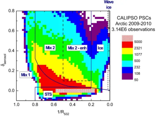
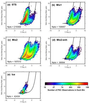
subsequently modified by Pitts et al. (2011) (hereafter referred to as P11), the CALIOP PSC algorithm now includes six composition classes: three classes of liquid/NAT mix-tures, with Mix1, Mix2, and Mix2-enhanced denoting increasingly higher NAT number density/volume; STS (which also includes low number densities of NAT particles whose optical signature is masked by the much more numerous STS droplets at cold

tem-5

peratures); H2O ice; and mountain wave ice, the latter having high particle number

densities (∼10 cm−3) but concomitantly small (1.0–1.5 µm radius) particles. Figure 1

shows a composite 2-D histogram of CALIOP PSC observations from the 2009–2010 Arctic winter in theδaerosol vs. 1/R532 coordinate system, with the boundaries of the

six composition classes denoted by the black lines. The boundaries drawn between

10

the composition classes are based on a limited set of optical calculations and, with the exception of the boundary separating STS from Mix1/Mix2/ice (P09), do not reflect the inherent uncertainty in the CALIOP measurements, especially inβperp. Hence, the

boundaries should be considered fuzzy, and “jumps” between adjacent composition classes occurring on small spatial scales may be simply a reflection of measurement

15

noise rather than a true change in cloud composition.

For this study, we have made a slight modification to the P09/P11 composition clas-sification scheme. PSC detection and composition clasclas-sification were done indepen-dently in the P09/P11 algorithm and, as a result, it is possible that a PSC may be detected through an enhancement inβperp, a clear indication of the presence of solid

20

particles, but the derivedδaerosolmay fall into the STS composition regime due to noise

in the calculated aerosol depolarization ratio. Similarly, a cloud may be detected strictly through an enhancement inR532(no detectable enhancement inβperp), yet the derived

δaerosolmay fall into one of the mixture regimes. Although this discrepancy only impacts

a very small fraction of PSC observations, it is straightforward to correct by including

25

two additional constraints to the P09/P11 composition classification scheme: (1) if a PSC is detected through an enhancement inβperp, it will be classified as a liquid/NAT

mixture or ice PSC (depending on the magnitude of R532) regardless of its derived

(7)

ACPD

12, 24643–24676, 2012

M. C. Pitts et al.

Title Page

Tables Figures

◭ ◮

Back Close

Full Screen / Esc

Discussion

P

a

per

|

Dis

cussion

P

a

per

|

Discussion

P

a

per

|

Discussio

n

P

a

per

PSC does not exhibit an enhancement inβperp, it will be classified as STS regardless

of its derivedδaerosol value.

Temperature profiles at each CALIOP measurement location are also included in the CALIOP Level 1 data files. The temperature data have been interpolated to the CALIOP Level 1 measurement locations from the Goddard Earth Observing System

5

Model, Version 5 (GEOS-5) six-hourly gridded analyses (Rienecker et al., 2008). To match the standard PSC grid, the GEOS-5 data are smoothed to the 5-km horizontal resolution and interpolated to the 180-m vertical grid.

2.2 Aura MLS

The Aura MLS detects thermal microwave emission from the Earth’s limb (Waters et

10

al., 2006) along the line-of-sight in the forward direction of the Aura spacecraft flight track. Vertical scans made from the Earth’s surface to a 90 km tangent height every 24.7 s provide a total of 3500 vertical profiles per day with a horizontal along track spacing of 1.5 degrees (165 km) and nearly global latitude coverage from 82◦_S–82◦_N.

The limb radiance measurements are inverted using a 2-D optimal estimation retrieval

15

(Livesey et al., 2006) to yield atmospheric profiles of temperature and composition in the vertical range 8–90 km (Livesey et al., 2006). The MLS version 3.3 measurements (Livesey et al., 2011) have typical single-profile precisions of 4–15 % for H₂O (Read et al., 2007; Lambert et al., 2007) and 0.7 ppbv for HNO3 (Santee et al., 2007). Vertical

and horizontal along-track resolutions are 3.1–3.5 km and 180–290 km for H2O, and

20

3.5–5.5 km and 400–550 km for HNO₃.

Since Aura flies in formation with CALIPSO in the A-train satellite constellation, CALIOP and MLS measurement tracks are closely aligned with spatial and tempo-ral di_fferences less than 10 km and 30 s after a repositioning of the Aura satellite in 2008 and about 200 km and 7–8 min. prior to 2008 (see Lambert et al., 2012).

25

(8)

ACPD

12, 24643–24676, 2012

M. C. Pitts et al.

Title Page

Tables Figures

◭ ◮

Back Close

Full Screen / Esc

Discussion

P

a

per

|

Dis

cussion

P

a

per

|

Discussion

P

a

per

|

Discussio

n

P

a

per

|

Meteorological Products (DMPs), such as equivalent latitude, are also mapped onto the PSC grid.

3 Data analyses

Our basic approach is to combine CALIOP PSC observations with nearly coincident Aura MLS gas species measurements and GEOS-5 temperature analyses to track the

5

uptake of gas phase HNO3 as a function of temperature. Comparing the observed

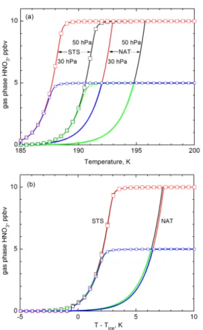
HNO₃uptake with theoretical equilibrium HNO₃uptake for NAT and STS indicates how well CALIOP PSCs in the various composition classes conform to expected tempera-ture existence regimes and also offers some insight into PSC growth kinetics. Figure 2 shows theoretical gas-phase HNO3 uptake curves assuming thermodynamic

equilib-10

rium conditions for STS (Carslaw et al., 1995) and NAT (Hanson and Mauersberger, 1988) at pressures of 30 and 50 hPa, assuming mixing ratios of 5 and 10 ppbv of total HNO3, 5 ppmv of H2O, and 0.1 ppbv H2SO4. The curves are presented as a function

of absolute temperature in Fig. 2a and as a function ofT−Tice in Fig. 2b, whereTiceis

the frost point temperature calculated using the Murphy and Koop (2005) relationship.

15

The figure illustrates clearly that in theT−Tice coordinate system, the individual curves

collapse into essentially single STS and NAT uptake curves, removing variations due to differences in atmospheric pressure level and local changes in H2O partial pressure

(Drdla et al., 2003).

For this assessment, we examined the CALIOP PSC data record from both polar

20

regions over the period from 2006 through 2011 and over a range of potential tem-perature levels spanning the 15–30 km altitude range. As will be discussed in Sect. 4, particle sedimentation and subsequent denitrification complicate the interpretation of the gas-phase HNO3 uptake and can also affect composition classification. As a

re-sult, data from the Antarctic, where the stratosphere is subject to severe denitrification

25

(9)

ACPD

12, 24643–24676, 2012

M. C. Pitts et al.

Title Page

Tables Figures

◭ ◮

Back Close

Full Screen / Esc

Discussion

P

a

per

|

Dis

cussion

P

a

per

|

Discussion

P

a

per

|

Discussio

n

P

a

per

complemented focused measurements from an extensive field campaign under the European Union RECONCILE (reconciliation of essential process parameters for an enhanced predictability of Arctic stratospheric ozone loss and its climate interactions) project conducted that winter from Kiruna, Sweden (P11; D ¨ornbrack et al., 2012). The 2009–2010 winter was characterized by unusually cold conditions in the stratosphere

5

from mid-December through January that resulted in widespread PSCs (D ¨ornbrack et al., 2012; P11, Khosrawi et al., 2011). The distribution of PSCs observed by CALIOP during the 2009–2010 winter (Fig. 1) spans nearly the entireδaerosol vs. 1/R532

mea-surement space with significant numbers of PSCs in all six composition classes, pro-viding an excellent dataset for assessing the robustness of our composition

classifi-10

cation. Although denitrification occurred during the 2009–2010 Arctic winter, average HNO3 abundances between 475–575 K potential temperature in January were close

to 10 ppbv (Khosrawi et al., 2011), our standard value for defining the composition boundaries. We will examine an Antarctic case later in the paper to illustrate how se-vere denitrification/dehydration impacts our composition classification.

15

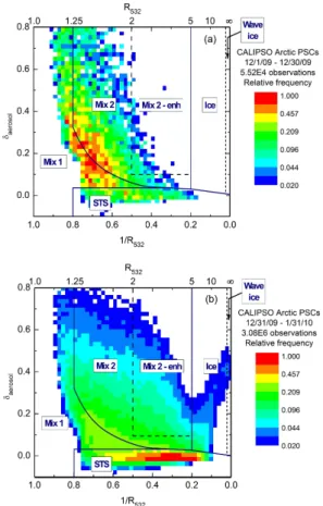
An interesting aspect of the 2009–2010 winter was the observation by CALIOP of tenuous liquid/NAT mixture PSCs with low NAT number densities in December, prior to the occurrence of ice (P11). These observations support the conclusions of Voigt et al. (2005) and Pagan et al. (2004) that ice nuclei are not a prerequisite for NAT PSC formation. To examine our classification scheme prior to the onset of denitrification, we

20

will analyse this period (1–30 December 2009) separately. The remainder of the PSC season (31 December 2009–31 January 2010) was characterized by extensive regions of PSCs in all composition classes. 2-D histograms of CALIOP PSC observations for these two periods are shown in Fig. 3.

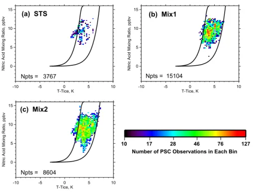
Figure 4 shows 2-D histograms of MLS HNO3uptake vs.T−Ticefor CALIOP PSC

ob-25

servations by composition class for 1–30 December at the 490 K potential temperature level (∼21 km).T is the ambient temperature at the CALIOP observation point (from

the GEOS-5 gridded analyses) and Tice is the frost point temperature (Murphy and

(10)

ACPD

12, 24643–24676, 2012

M. C. Pitts et al.

Title Page

Tables Figures

◭ ◮

Back Close

Full Screen / Esc

Discussion

P

a

per

|

Dis

cussion

P

a

per

|

Discussion

P

a

per

|

Discussio

n

P

a

per

|

a guide for the reader’s eye, reference equilibrium uptake curves for STS and NAT are overlaid in the figures assuming total abundances of 16 ppbv HNO3and 5 ppmv H2O,

which are representative of early season values at this level. As vortex temperatures fell below NAT equilibrium during mid-December, tenuous NAT mixture clouds were observed, with some indication of STS clouds on the coldest days. No ice or Mix2-enh

5

PSCs were observed during this period. The majority of Mix1 and Mix2 PSC observa-tions are in an uptake regime that falls between the reference NAT and STS equilibrium uptake curves at temperatures betweenTice+1 K andTice+7 K, with a larger range of

HNO3 uptake occurring on Mix2 particles. The observed uptake suggests that these

non-equilibrium NAT mixtures have been exposed to temperatures belowT_NATfor

mod-10

erate time periods, but not long enough for the NAT particles to reach thermodynamic equilibrium. The limited number of STS observations during this period is not sufficient to adequately assess this composition class at this time.

Histograms of HNO₃ uptake as a function of T−Tice for 31 December–31 January

are shown in Fig. 5. PSCs in all composition classes were observed during this period.

15

Most observations in the STS class (Fig. 5a) are clearly aligned with the reference STS equilibrium uptake curve, as would be anticipated since STS particles are thought to grow fast enough to maintain equilibrium with the gas phase HNO3. The main STS data

cluster does lie at slightly lower temperatures than the reference equilibrium curve, a finding consistent with Lambert et al. (2012). Also of note is the secondary family of

20

STS observations that lie along the reference NAT equilibrium uptake curve at tem-peratures too warm to support STS existence. These points are classified as STS because they do not exhibit a detectable enhancement in perpendicular backscatter, which would signal the presence of solid particles. An example of points classified as STS but at anomalously warm temperatures is shown in Fig. 6 for a PSC observed by

25

(11)

ACPD

12, 24643–24676, 2012

M. C. Pitts et al.

Title Page

Tables Figures

◭ ◮

Back Close

Full Screen / Esc

Discussion

P

a

per

|

Dis

cussion

P

a

per

|

Discussion

P

a

per

|

Discussio

n

P

a

per

observed perpendicular backscatter signal, which lowers the measured perpendicular backscatter to values below our detection threshold for NAT particles. Hereafter we re-fer to this noise-induced misclassification as “speckle” based on how it manifests itself in CALIOP PSC images. For the 2009–2010 winter, we estimate that approximately 6 % of all measurements classified as STS are likely NAT mixtures misclassified due

5

to speckle. Similar noise-induced misclassification likely occurs to some degree in all composition classes, but is only detectable when the misclassification puts the com-position in an unexpected temperature regime. It may be possible to eliminate speckle by applying a spatial filter that assumes composition homogeneity over appropriately small spatial scales. This will be investigated for our next generation algorithm.

10

The HNO₃ uptake as a function ofT−Tice for PSCs identified as NAT mixtures by

our composition classification scheme are shown in Fig. 5b–d. The mixture observa-tions cover a broad range of temperatures from 7–8 K above the frost point to near the frost point. The uptake of HNO₃ for each of the mixture classes has two distinct modes: one closely aligned with the STS equilibrium curve and another aligned with

15

the NAT equilibrium curve, but there are also numerous points falling in between the two reference curves. At first glance, the mixture points that exhibit HNO₃uptake sim-ilar to STS may appear to be misclassified STS. However, these points actually rep-resent STS/NAT mixtures in which the uptake of HNO3 by the relatively low number

density NAT particles is a slow process, whereas HNO3 condensation on the much

20

more numerous liquid droplets occurs rapidly in response to decreases in temperature. In these mixture cases, the presence of the NAT particles produces a detectable en-hancement in the CALIOP perpendicular backscatter signal, hence their classification as NAT mixtures, but at colder temperatures the more numerous liquid droplets dom-inate the uptake of HNO3. For these mixtures, the CALIOP perpendicular backscatter

25

(12)

ACPD

12, 24643–24676, 2012

M. C. Pitts et al.

Title Page

Tables Figures

◭ ◮

Back Close

Full Screen / Esc

Discussion

P

a

per

|

Dis

cussion

P

a

per

|

Discussion

P

a

per

|

Discussio

n

P

a

per

|

of time, allowing a larger fraction of the gas phase HNO₃ to condense onto the NAT particles and bringing the mixture closer to thermodynamic equilibrium.

The HNO3uptake for observations identified as ice PSCs during this period is shown

in Fig. 5e. Ice PSCs are expected to occur only at temperatures below the frost point, with almost complete uptake of gas-phase HNO3 by STS (or NAT) prior to the

tem-5

perature having reached the frost point. In the CALIOP observations, there is a clear maximum in ice PSCs at temperatures near or below the frost point and HNO₃values below 2 ppbv, but ice observations also extend to temperatures above the frost point and larger HNO3abundances. Although this would appear to be a misclassification, i.e.

ice PSCs occurring at temperatures outside their expected thermodynamic existence

10

regime, we are confident that the ice classification is correct since the large optical sig-nal (bothR532andβperp) produced by ice PSCs is a robust signature. The anomalous

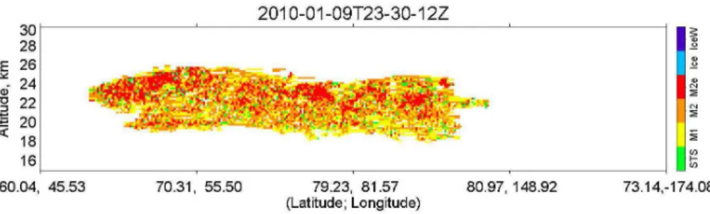
points in Fig. 5e are likely caused by differences in measurement resolution among CALIOP, GEOS-5, and MLS. During the first half of this period (31 December–14 Jan-uary), the vast majority of ice PSCs were associated with orographic wave events that

15

occurred on relatively small spatial scales (e.g., P11). With the high spatial resolution sampling of CALIOP and the inherently large scattering ratio values associated with ice PSCs, mountain wave ice PSCs are easily detected and properly classified by CALIOP at the highest PSC resolution (5 km × 180 m). However, given the relatively coarse

resolution of both the GEOS-5 gridded analyses (0.5 degrees) and Aura MLS HNO₃

20

measurements (400–550 km horizontal× 3.5–5.5 km vertical), small scale wave

fea-tures are more difficult to fully resolve. The amplitude of the temperature perturbations associated with these waves is typically underestimated in the GEOS-5 gridded anal-yses, and the localized uptake of HNO3 by the STS in the cold phase of the waves

will be underestimated by MLS. To illustrate this point further, gas-phase HNO3uptake

25

associated with CALIOP ice PSCs for the two distinct periods are shown in Fig. 7. The ice observations at anomalously warm temperatures and relatively large HNO3mixing

(13)

ACPD

12, 24643–24676, 2012

M. C. Pitts et al.

Title Page

Tables Figures

◭ ◮

Back Close

Full Screen / Esc

Discussion

P

a

per

|

Dis

cussion

P

a

per

|

Discussion

P

a

per

|

Discussio

n

P

a

per

PSCs were observed on much larger spatial scales associated with synoptic-scale re-gions of temperatures below the frost point, and both GEOS-5 and MLS are able to better resolve such features.

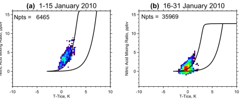
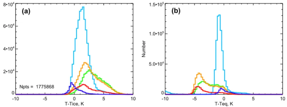
Histograms of PSC occurrence vs.T−TiceandT−Teq for 31 December 2009–31

Jan-uary 2010 are depicted in Fig. 8 for all CALIOP composition classes shown in Fig. 5.

5

Teq is defined asTice,TNAT, orTSTS, depending on the PSC composition classification,

and is calculated using the Murphy and Koop (2005) (T_ice), Hanson and Mauersberger (1988) (TNAT), and Carslaw et al. (1995) (TSTS) relationships with the coincident MLS

HNO3 and H2O abundances. For compositions other than ice, the histograms are

re-stricted to observations with HNO₃values greater than 1 ppbv to avoid the region where

10

the NAT and STS equilibrium curves converge. To a large degree, observations in each composition class conform to their expected temperature existence regimes, except for the points misclassified as STS at too warm temperatures (speckle) and the warm-biased ice PSCs associated with small-scale orographic waves. Ignoring the positive tail in the distribution of STS observations due to speckle, STS PSCs occur over a

15

relative narrow temperature range centered about 1 K below the STS equilibrium tem-perature. The peak at 1 K below equilibrium may be an indication of a cold bias in the GEOS-5 temperature analyses as noted by Lambert et al. (2012). The distribution of each NAT mixture class has a bimodal appearance with one mode near the NAT equi-librium temperature and a second, more populous mode at 4-5 K below NAT equiequi-librium

20

– which is very near the STS mode inT−Ticespace (Fig. 8a). This more populous mode

is far out of equilibrium with respect to NAT and corresponds to mixtures with NAT par-ticles producing a large enough perpendicular backscatter signal to be detectable by CALIOP, but whose gas-phase HNO3 uptake is dominated by the much more

numer-ous STS droplets. The fact that the NAT mixture histograms are distinctly bimodal, i.e.

25

the mixtures do not occur uniformly over the space between TNAT and TSTS, is quite

interesting and may indicate a rapid switch from the thermodynamically metastable STS to stable NAT after sufficient exposure of air parcels to temperatures below TNAT.

(14)

ACPD

12, 24643–24676, 2012

M. C. Pitts et al.

Title Page

Tables Figures

◭ ◮

Back Close

Full Screen / Esc

Discussion

P

a

per

|

Dis

cussion

P

a

per

|

Discussion

P

a

per

|

Discussio

n

P

a

per

|

frost point (also consistent with Lambert et al., 2012) with a full-width-half-maximum of about 1.5 K. The longer positive tail in the ice PSC distribution is due to warm biased temperatures associated with the wave ice events.

Histograms of PSC occurrence vs.T−Tice andT−Teq for five seasons in the Arctic

(2006–2011) are shown in Fig. 9. These multi-year histograms are similar in nature to

5

as those for the 2009–10 Arctic season (Fig. 8), with observations in all composition classes conforming to expected thermodynamic existence regimes. The notable ex-ceptions again are observations classified as STS at anomalously warm temperatures, which are likely NAT clouds misclassified due to noise in βperp (speckle) and the ice

PSCs at (apparent) temperatures above the frost point, which are associated with

oro-10

graphic waves, the predominant mechanism for ice PSC formation in the Arctic. Com-position classification is also robust in the Antarctic, as illustrated by the histograms of PSC occurrence vs.T−Tice and T−Teq for six seasons in the Antarctic (2006–2011)

in Fig. 10. Although less pronounced in than in the Arctic, a small number of anoma-lously warm STS points also appear in the Antarctic STS histogram. Ice PSC formation

15

in the Antarctic occurs more frequently and generally on larger spatial scales than in the Arctic and as a consequence the number of ice PSCs at (apparent) temperatures above the frost point are less common. These multi-year histograms represent over 1.7 million Arctic and 10.1 million Antarctic PSC observations and provide compelling evidence that the P09/P11 composition classification is robust.

20

4 Impact of denitrification on composition classification

The composition class boundaries defined by P09 and P11 are based on a standard set of conditions: 50 hPa atmospheric pressure and nominal mixing ratios of 10 ppbv HNO3and 5 ppmv H2O. For most Arctic winters and early in the Antarctic winter, these

values are representative. However, the Antarctic is subject to severe denitrification

25

(15)

ACPD

12, 24643–24676, 2012

M. C. Pitts et al.

Title Page

Tables Figures

◭ ◮

Back Close

Full Screen / Esc

Discussion

P

a

per

|

Dis

cussion

P

a

per

|

Discussion

P

a

per

|

Discussio

n

P

a

per

on the composition class boundaries. Shown in Fig. 11a are theoretical calculations of CALIOP optical signals for various liquid/NAT mixtures and ice computed for the standard conditions (10 ppbv HNO3). The ice PSCs are the arm of points extending

up and to the right from the STS domain at 1/R532 ∼0.2. For comparison, Fig. 11b

depicts theoretical calculations for denitrified conditions of 5 ppbv HNO3. The reduction

5

in available condensable HNO3 limits the growth potential of the particles, resulting

in a systematic shift of the optical signals to smaller scattering ratios (larger 1/R₅₃₂) values. For these conditions, the arm of ice points is shifted to the left and departs from the STS domain at 1/R532∼0.3. Therefore, to properly account for denitrification

in our composition classification scheme, the boundary between ice and NAT mixture

10

(Mix2 and Mix2-enh) PSC domains should shifted to smaller scattering ratio values (larger 1/R532 values). The magnitude of the shift is a function of the total abundance

of HNO3.

The e_ffects of denitrification can also clearly be seen in the CALIOP PSC observa-tions. For example, shown in Fig. 12a is the distribution of PSCs observed by CALIOP

15

for June 2009 in an equivalent latitude band between 60◦_{S and 70}◦_{S. The total HNO}

3

mixing ratio during June was decreasing as denitrification began, but on average was close to our standard value of 10 ppbv. The period was dominated by fully developed STS (maximum along theδaerosol=0 axis) and ice PSCs, with a small number of

mix-tures. Similar to the theoretical calculations (Fig. 11a), the arm of ice PSC observations

20

(dashed white line) departs from the STS maximum at 1/R532 values of 0.2. In

con-trast, Fig. 12b depicts CALIOP observations in August 2009 deep inside the vortex at equivalent latitudes between 75◦_{S and 90}◦_{S. The total HNO}

3 abundance at this time

had dropped significantly from early season values to around 5 ppbv or less resulting in a discernible shift in the point where the axis of the ice arm departs from the STS

25

mode, to a 1/R532value of about 0.3 (similar to Fig. 11b).

(16)

ACPD

12, 24643–24676, 2012

M. C. Pitts et al.

Title Page

Tables Figures

◭ ◮

Back Close

Full Screen / Esc

Discussion

P

a

per

|

Dis

cussion

P

a

per

|

Discussion

P

a

per

|

Discussio

n

P

a

per

|

Mix2 PSC observations from the Antarctic during August 2009, when denitrification is severe. Histograms of ice and Mix2-enh PSC occurrence as a function of T−Tice

from the interior of the vortex in August 2009 are shown in Fig. 13. Figure 13a depicts histograms for composition classification using our standard ice/Mix2-enh boundary (1/R532=0.2). With random measurement noise and no bias in temperature andTice,

5

one would expect the ice PSC histogram to be Gaussian with a mode atT−Tice=0. The

mode of the actual histogram is slightly below the frost point, but the positive tail of the distribution appears to be truncated relative to the negative tail. The Mix2-enh distribu-tion also has a maximum near the frost point, some of which may be misclassified ice, but also extends to warmer temperatures as would be expected for NAT mixtures. To

10

account for denitrification in our composition classification, we should shift the composi-tion boundaries appropriately based on the total abundance of HNO3. To demonstrate

this, Fig. 13b shows histograms for composition classification using an ice/mix2-enh boundary of 1/R532=0.3. For this case, there has been a redistribution of

composi-tions with over a 50 % increase in the number of ice clouds which had been classified

15

as Mix2-enh in our standard case. The shape of the ice PSC distribution in this case appears to be more Gaussian-like than in the standard case, with no obvious trun-cation of the positive tail. Figure 13c shows histograms for composition classifitrun-cation using an ice/mix2-enh boundary of 1/R532=0.4. This results in more than a doubling

of the number of ice PSCs relative to the standard case, but the ice PSC distribution

20

now shows a noticeable extension to warmer temperatures (Tice+3 K), indicating that

the boundary has been shifted too far to the left and with some Mix2-enh clouds now being misclassified as ice. In practice, it will be di_fficult to accurately account for the magnitude of denitrification since most HNO3measurements are gas phase only and

are impacted by uptake on PSC particles.

(17)

ACPD

12, 24643–24676, 2012

M. C. Pitts et al.

Title Page

Tables Figures

◭ ◮

Back Close

Full Screen / Esc

Discussion

P

a

per

|

Dis

cussion

P

a

per

|

Discussion

P

a

per

|

Discussio

n

P

a

per

5 Summary and future direction

We have used Aura MLS gas phase HNO3and H2O measurements along with GEOS-5

temperature analyses to independently assess the CALIOP PSC composition classifi-cation scheme, which is based solely on the lidar optical measurements. Our approach was to examine the uptake of HNO3 as a function of T−Tice to determine if the

as-5

signed PSC composition is consistent with the thermodynamic existence regimes for STS, NAT, and ice. The results indicate that, overall, the CALIOP PSC composition classification performance is excellent with each class exhibiting uptake behavior con-sistent with theoretical expectations.

PSCs identified as STS exhibit gas phase uptake of HNO₃ consistent with theory,

10

but with a small temperature bias, consistent with previous studies. Some (∼6 %) of

points being classified as STS are actually liquid/NAT mixtures being misclassified due to the so-called speckle e_ffect caused by pixel-scale negative noise excursions in the CALIOP perpendicular backscatter measurements. Although not detectable in these analyses, misclassification due to such speckle likely occurs at a similar rate in other

15

composition classes.

PSCs identified as liquid/NAT mixtures exhibit two distinct preferred modes. One such mode is significantly out of thermodynamic equilibrium with respect to NAT (4– 5 K belowTNAT), with HNO3 uptake dominated by the more numerous liquid droplets.

The other liquid/NAT mode is much closer to NAT thermodynamic equilibrium indicating

20

that the particles have been exposed to temperatures belowTNAT for extended periods

of time.

Ice PSC classification is robust in the CALIOP optical data, and the mode in the ice observations occurs about 0.5 K below the frost point. The anomalously warm tem-peratures and high HNO₃values associated with CALIOP observations of small-scale

25

(18)

ACPD

12, 24643–24676, 2012

M. C. Pitts et al.

Title Page

Tables Figures

◭ ◮

Back Close

Full Screen / Esc

Discussion

P

a

per

|

Dis

cussion

P

a

per

|

Discussion

P

a

per

|

Discussio

n

P

a

per

|

We also demonstrated that severe denitrification can impact the CALIOP compo-sition classification. The P09/P11 compocompo-sition class boundaries are based on nomi-nal vapor abundances, and during periods of severe denitrification these boundaries should be adjusted to account for the reduced growth potential of the PSC particles. The biggest impact is a shift in the boundary between ice PSCs and NAT mixtures. As

5

a result, some ice PSCs are being misclassified as NAT mixtures using the P09/P11 scheme during periods of moderate to severe denitrification, primarily in the Antarctic. We will investigate methods to correct these deficiencies for our next generation algorithm.

Acknowledgements. The Aura MLS gas species data and Derived Meteorological Products

10

(DMP) were provided courtesy of the MLS team and obtained through the Aura MLS web-site (http://mls.jpl.nasa.gov/index-eos-mls.php). We would also like to thank David Considine, Program Scientist for the CALIPSO/CloudSat Missions for continued support of this research. Support for L. Poole is provided under NASA contract NNL11AA10D. Work at the Jet Propul-sion Laboratory, California Institute of Technology, was carried out under a contract with the

15

National Aeronautics and Space Administration.

References

Biele, J., Tsias, A., Luo, B. P., Carslaw, K. S., Neuber, R., Beyerle, G., and Peter, T.: Nonequi-librium coexistence of solid and liquid particles in Arctic stratospheric clouds, J. Geophys. Res., 106, 22991–23007, 2001.

20

Cairo, F., Di Donfrancesco, G., Adriani, A., Pulvirenti, L., and Fierli, F.: Comparison of various linear depolarization parameters measured by lidar, Appl. Opt., 38, 4425–4432, 1999. Carslaw, K. S., Luo, B. P., and Peter, T.: An analytic expression for the composition of aqueous

HNO₃-H₂SO₄stratospheric aerosols including gas phase removal of HNO₃, Geophys. Res. Lett., 22, 1877–1880, 1995.

25

(19)

ACPD

12, 24643–24676, 2012

M. C. Pitts et al.

Title Page

Tables Figures

◭ ◮

Back Close

Full Screen / Esc

Discussion

P

a

per

|

Dis

cussion

P

a

per

|

Discussion

P

a

per

|

Discussio

n

P

a

per

H ¨opfner, M., Pitts, M. C., and Poole, L. R.: Comparison between CALIPSO and MI-PAS observations of polar stratospheric clouds, J. Geophys. Res., 114, D00H05, doi:10.1029/2009JD012114, 2009.

Hunt, W. H., Winker, D. M., Vaughan, M. A., Powell, K. A., Lucker, P. L., and Weimer, C.: CALIPSO Lidar Description and Performance Assessment, J. Atmos. Oceanic Technol., 26,

5

1214–1228, doi:10.1175/2009JTECHA1223.1, 2009.

Khosrawi, F., Urban, J., Pitts, M. C., Voelger, P., Achtert, P., Kaphlanov, M., Santee, M. L., Manney, G. L., Murtagh, D., and Fricke, K.-H.: Denitrification and polar stratospheric cloud formation during the Arctic winter 2009/2010, Atmos. Chem. Phys., 11, 8471–8487, doi:10.5194/acp-11-8471-2011, 2011.

10

Lambert, A., Read, W. G., Livesey, N. J., Santee, M. L., Manney, G. L., Froidevaux, L., Wu, D. L., Schwartz, M. J., Pumphrey, H. C., Jimenez, C., Nedoluha, G. E., Cofield, R. E., Cuddy, D. T., Daffer, W. H., Drouin, B. J., Fuller, R. A., Jarnot, R. F., Knosp, B. W., Pickett, H. M., Perun, V. S., Snyder, W. V., Stek, P. C., Thurstans, R. P., Wagner, P. A., Waters, J. W., Jucks, K. W., Toon, G. C., Stachnik, R. A., Bernath, P. F., Boone, C. D., Walker, K. A., Urban, J.,

15

Murtagh, D., Elkins, J. W., and Atlas, E.: Validation of the Aura Microwave Limb Sounder middle atmosphere water vapor and nitrous oxide measurements, J. Geophys. Res., 112, D24S36, doi:10.1029/2007JD008724, 2007.

Lambert, A., Santee, M. L., Wu, D. L., and Chae, J. H.: A-train CALIOP and MLS observations of early winter Antarctic polar stratospheric clouds and nitric acid in 2008, Atmos. Chem.

20

Phys., 12, 2899–2931, doi:10.5194/acp-12-2899-2012, 2012.

Livesey, N. J., Snyder, W. V., Read, W. G., and Wagner, P. A.: Retrieval algorithms for the EOS Microwave Limb Sounder (MLS), IEEE T. Geosci. Remote, 44, 1144–1155, 2006.

Livesey, N. J., Read, W. G., Froidevaux, L., Lambert, A., Manney, G. L., Pumphrey, H. C., Santee, M. L., Schwartz, M. J., Wang, S., Cofield, R. E., Cuddy, D. T., Fuller, R. A., Jarnot,

25

R. F., Jiang, J. H., Knosp, B. W., Stek, P. C., Wagner, P. A., and Wu, D. L.: Version 3.3 Level 3 data quality and description document, Tech. Rep. JPL D-33509, Jet Propulsion Laboratory, available at: http://mls.jpl.nasa.gov (last access: October 2011), 2011.

Lowe, D. and A. R. MacKenzie, Polar stratospheric cloud microphysics and chemistry, J. Atmos. Solar-Terr. Phys., 70, 13–40, 2008.

30

(20)

ACPD

12, 24643–24676, 2012

M. C. Pitts et al.

Title Page

Tables Figures

◭ ◮

Back Close

Full Screen / Esc

Discussion

P

a

per

|

Dis

cussion

P

a

per

|

Discussion

P

a

per

|

Discussio

n

P

a

per

|

Noel, V. and Pitts, M.: Gravity wave events from mesoscale simulations compared to polar stratospheric clouds observed from spaceborne lidar over the Antarctic Peninsula, J. Geo-phys. Res., 117, D11207, doi:10.1029/2011JD017318, 2012.

Noel, V., Hertzog, A., Chepfer, H., and Winker, D., Polar stratospheric clouds over Antarctica from the CALIPSO spaceborne lidar, J. Geophys. Res., 113, D02205,

5

doi:10.1029/2007JD008616, 2008.

Pagan, K. L., Tabazadeh, A., Drdla, K., Hervig, M. E., Eckermann, S. D., Browell, E. V., Legg, M. J., and Foschi, P. G.: Observational evidence against mountain-wave generation of ice nuclei as a prerequisite for the formation of three solid nitric acid polar stratospheric clouds observed in the Arctic in early December 1999, J. Geophys. Res., 109, D04312,

10

doi:1029/2003JD003846, 2004.

Pitts, M. C., Thomason, L. W., Poole, L. R., and Winker, D. M.: Characterization of Polar Strato-spheric Clouds with spaceborne lidar: CALIPSO and the 2006 Antarctic season, Atmos. Chem. Phys., 7, 5207–5228, doi:10.5194/acp-7-5207-2007, 2007.

Pitts, M. C., Poole, L. R., and Thomason, L. W.: CALIPSO polar stratospheric cloud

observa-15

tions: second-generation detection algorithm and composition discrimination, Atmos. Chem. Phys., 9, 7577–7589, doi:10.5194/acp-9-7577-2009, 2009.

Pitts, M. C., Poole, L. R., D ¨ornbrack, A., and Thomason, L. W.: The 2009–2010 Arctic polar stratospheric cloud season: a CALIPSO perspective, Atmos. Chem. Phys., 11, 2161–2177, doi:10.5194/acp-11-2161-2011, 2011.

20

Powell, K. A., Hostetler, C. A., Liu, Z., Vaughan, M. A., Kuehn, R. E., Hunt, W. H., Lee, K., Trepte, C. R., Rogers, R. R., Young, S. A., and Winker, D. M.: CALIPSO Lidar Calibration Algorithms: Part I – Nighttime 532 nm Parallel Channel and 532 nm Perpendicular Channel, J. Atmos. Oceanic Technol., 26, 2015–2033, doi:10.1175/2009JTECHA1242.1, 2009. Read, W. G., Lambert, A., Bacmeister, J., Cofield, R. E., Christensen, L. E., Cuddy, D. T., Daffer,

25

W. H., Drouin, B. J., Fetzer, E., Froidevaux, L., Fuller, R., Herman, R., Jarnot, R. F., Jiang, J. H., Jiang, Y. B., Kelly, K., Knosp, B. W., Kovalenko, L. J., Livesey, N. J., Liu, H. C., Manney, G. L., Pickett, H. M., Pumphrey, H. C., Rosenlof, K. H., Sabounchi, X., Santee, M. L., Schwartz, M. J., Snyder,W. V., Stek, P. C., Su, H., Takacs, L. L., Thurstans, R. P., Vomel, H., Wagner, P. A., Waters, J.W.,Webster, C. R.,Weinstock, E. M., and Wu, D. L.: Aura Microwave Limb

30

(21)

ACPD

12, 24643–24676, 2012

M. C. Pitts et al.

Title Page

Tables Figures

◭ ◮

Back Close

Full Screen / Esc

Discussion

P

a

per

|

Dis

cussion

P

a

per

|

Discussion

P

a

per

|

Discussio

n

P

a

per

Santee, M. L., Lambert, A., Read, W. G., Livesey, N. J., Cofield, R. E., Cuddy, D. T., Daffer, W. H., Drouin, B. J., Froidevaux, L., Fuller, R. A., Jarnot, R. F., Knosp, B. W., Manney, G. L., Perun, V. S., Snyder, W. V., Stek, P. C., Thurstans, R. P., Wagner, P. A., Waters, J. W., Muscari, G., de Zafra, R. L., Dibb, J. E., Fahey, D.W., Popp, P. J., Marcy, T. P., Jucks, K. W., Toon, G. C., Stachnik, R. A., Bernath, P. F., Boone, C. D., Walker, K. A., Urban, J., and Murtagh, D.:

5

Validation of the Aura Microwave Limb Sounder HNO₃ measurements, J. Geophys. Res., 112, D24S40, doi:10.1029/2007JD008721, 2007.

Solomon, S.: Stratospheric ozone depletion: A review of concepts and history, Rev. Geophys., 37, 275–316, 1999.

Stephens, G. L., Vane, D. G., Boain, R. J., Mace, G. G., Sassen, K., Wang, Z., Illingworth, A.

10

J., O’Connor, E. J., Rossow, W. B., Durden, S. L., Miller, S. D., Austin, R. T., Benedetti, A., Mitrescu, C., and the CloudSat Science Team: The CloudSat mission and the A-Train: A new dimension of space-based observations of clouds and precipitation, B. Am. Meteorol. Soc., 83, 1771–1790, 2002.

Toon, O., Tabazadeh, A., Browell, E., and Jordan, J.: Analysis of lidar observations of Arctic

15

polar stratospheric clouds during January 1989, J. Geophys. Res., 105, 20589–20615, 2000. Voigt, C., Schlager, H., Luo, B. P., D ¨ornbrack, A., Roiger, A., Stock, P., Curtius, J., V ¨ossing,

H., Borrmann, S., Davies, S., Konopka, P., Schiller, C., Shur, G., and Peter, T.: Nitric Acid Trihydrate (NAT) formation at low NAT supersaturation in Polar Stratospheric Clouds (PSCs), Atmos. Chem. Phys., 5, 1371–1380, doi:10.5194/acp-5-1371-2005, 2005

20

Waters, J. W., Froidevaux, L., Harwood, R. S., Jarnot, R. F., Pickett, H. M., Read, W. G., Siegel, P. H., Cofield, R. E., Filipiak, M. J., Flower, D. A., Holden, J. R., Lau, G. K. K., Livesey, N. J., Manney, G. L., Pumphrey, H. C., Santee, M. L., Wu, D. L., Cuddy, D. T., Lay, R. R., Loo, M. S., Perun, V. S., Schwartz, M. J., Stek, P. C., Thurstans, R. P., Boyles, M. A., Chandra, K. M., Chavez, M. C., Chen, G. S., Chudasama, B. V., Dodge, R., Fuller, R. A., Girard, M. A.,

25

Jiang, J. H., Jiang, Y. B., Oswald, J. E., Patel, N. C., Pukala, D. M., Quintero, O., Scaff, D., Van Snyder, W., Tope, M. C., Wagner, P. A., and Walch, M. J.: The Earth Observing System Microwave Limb Sounder (EOS MLS) on the Aura satellite, IEEE T. Geosci. Remote, 44, 1075–1092, 2006.

Winker, D. M., Vaughan, M. A., Omar, A. H., Hu, Y., Powell, K. A., Liu, Z., Hunt, W. H., and

30

(22)

ACPD

12, 24643–24676, 2012

M. C. Pitts et al.

Title Page

Tables Figures

◭ ◮

Back Close

Full Screen / Esc

Discussion

P

a

per

|

Dis

cussion

P

a

per

|

Discussion

P

a

per

|

Discussio

n

P

a

per

|

Fig. 1.Composite 2-D histogram of all CALIOP PSC observations during the 2009–2010 Arc-tic winter in theδ_aerosol vs. 1/R₅₃₂ coordinate system, with the solid black lines denoting the boundaries of the six PSC composition domains defined by P09 and the dashed boxes denot-ing the domains of the two new composition sub-classes defined by P11. The histogram bin size is 0.02×0.02 (both unitless) and the color scale indicates the number of cloud observations

(23)

ACPD

12, 24643–24676, 2012

M. C. Pitts et al.

Title Page

Tables Figures

◭ ◮

Back Close

Full Screen / Esc

Discussion

P

a

per

|

Dis

cussion

P

a

per

|

Discussion

P

a

per

|

Discussio

n

P

a

per

Fig. 2.Theoretical equilibrium uptake of HNO₃by STS (square symbols) and NAT as a function of(a)temperature and(b)T−Tice. Red and black curves/symbols: 10 ppbv HNO3, 5 ppmv H2O;

(24)

ACPD

12, 24643–24676, 2012

M. C. Pitts et al.

Title Page

Tables Figures

◭ ◮

Back Close

Full Screen / Esc

Discussion

P

a

per

|

Dis

cussion

P

a

per

|

Discussion

P

a

per

|

Discussio

n

P

a

per

|

Fig. 3.Composite 2-D histogram of all CALIOP PSC observations for two periods of the 2009– 2010 Arctic winter over the altitude range from 15–30 km in theδaerosol vs. 1/R532 coordinate

(25)

ACPD

12, 24643–24676, 2012

M. C. Pitts et al.

Title Page Abstract Introduction Conclusions References Tables Figures ◭ ◮ ◭ ◮ Back Close

Full Screen / Esc

Printer-friendly Version Interactive Discussion Discussion P a per | Dis cussion P a per | Discussion P a per | Discussio n P a per 0 1

- -5 0 5 10

0 5 0 1 5 1

Nitric Acid Mixing Ratio, ppbv

7 6 7 3 = s t p N 0 1

- -5 0 5 10

K , e c i T -T 0 5 0 1 5 1

4 0 1 5 1 = s t p N 0 1

- -5 0 5 10

K , e c i T -T 0 5 0 1 5 1

4 0 6 8 = s t p N

Number of PSC Observations in Each Bin 10 17 28 46 76 127

(a) STS (b) Mix1

(c) Mix2

K , e c i T -T

Fig. 4.Uptake of nitric acid as a function ofT−Ticefor CALIOP Arctic PSC observations at 490 K

potential temperature during 1–30 December 2009 for(a)STS,(b)Mix1, and(c)Mix2 clouds. The histogram bin size is 0.25 ppbv×0.25 K and the color scale indicates the number of cloud

(26)

ACPD

12, 24643–24676, 2012

M. C. Pitts et al.

Full Screen / Esc

Printer-friendly Version Interactive Discussion Discussion P a per | Dis cussion P a per | Discussion P a per | Discussio n P a per | 0 1

- -5 0 5 10

K , e c i T -T 0 5 0 1 5 1

9 6 3 9 1 2 = s t p N 0 1

- -5 0 5 10

K , e c i T -T 0 5 0 1 5 1

7 5 9 8 5 1 = s t p N 0 1

- -5 0 5 10

K , e c i T -T 0 5 0 1 5 1

0 1 0 7 9 1 = s t p N 0 1

- -5 0 5 10

K , e c i T -T 0 5 0 1 5 1

4 6 0 8 6 = s t p N 0 1

- -5 0 5 10

K , e c i T -T 0 5 0 1 5 1

4 3 4 2 4 = s t p N

Number of PSC Observations in Each Bin 10 27 74 203 552 1505

(a) STS (b) Mix1

(c) Mix2 (d) Mix2-enh

(e) Ice

Fig. 5.Uptake of nitric acid as a function of T−Tice for CALIOP Arctic PSC observations at

490 K potential temperature during 31 December 2009–31 January 2010 for(a)STS,(b)Mix 1,(c)Mix 2,(d)Mix 2-enh, and(e)ice clouds. The histogram bin size is 0.25 ppbv×0.25 K and

(27)

ACPD

12, 24643–24676, 2012

M. C. Pitts et al.

Title Page

Tables Figures

◭ ◮

Back Close

Full Screen / Esc

Discussion

P

a

per

|

Dis

cussion

P

a

per

|

Discussion

P

a

per

|

Discussio

n

P

a

per

(28)

ACPD

12, 24643–24676, 2012

M. C. Pitts et al.

Title Page

Tables Figures

◭ ◮

Back Close

Full Screen / Esc

Discussion

P

a

per

|

Dis

cussion

P

a

per

|

Discussion

P

a

per

|

Discussio

n

P

a

per

|

0 1

- -5 0 5 10

K , e c i T -T 0

5 0 1

5 1

5 6 4 6 = s t p N

0 1

- -5 0 5 10

K , e c i T -T 0

5 0 1

5 1

9 6 9 5 3 = s t p N

(a) 1-15 January 2010 (b) 16-31 January 2010

Fig. 7.HNO₃uptake as a function ofT−Tice for CALIOP ice PSC observations during(a) 1–

(29)

ACPD

12, 24643–24676, 2012

M. C. Pitts et al.

Title Page

Tables Figures

◭ ◮

Back Close

Full Screen / Esc

Discussion

P

a

per

|

Dis

cussion

P

a

per

|

Discussion

P

a

per

|

Discussio

n

P

a

per

5

- 0 5 10

K , e c i T -T 0

0 1 • 0 .

5 3

0 1 • 0 .

1 4

0 1 • 5 .

1 4

Number

5

- 0 5 10

K , q e T -T 0

0 1 • 0 .

5 3

0 1 • 0 .

1 4

0 1 • 5 .

1 4

0 1 • 0 .

2 4

0 1 • 5 .

2 4

0 1 • 0 .

3 4

Number

(a) (b)

Fig. 8. Histograms of CALIOP PSC observations at 490 K potential temperature during 31 December 2009–31 January 2010 as a function of(a)T−Tice and(b)T−Teqby composition:

(30)

ACPD

12, 24643–24676, 2012

M. C. Pitts et al.

Title Page

Tables Figures

◭ ◮

Back Close

Full Screen / Esc

Discussion

P

a

per

|

Dis

cussion

P

a

per

|

Discussion

P

a

per

|

Discussio

n

P

a

per

|

0 1

- -5 0 5 10

K , e c i T -T 0

0 1 •

2 4

0 1 •

4 4

0 1 •

6 4

0 1 •

8 4

Number

8 6 8 5 7 7 1 = s t p N

0 1

- -5 0 5 10

K , q e T -T 0

0 1 • 0 .

5 4

0 1 • 0 .

1 5

0 1 • 5 .

1 5

Number

(a) (b)

Fig. 9.Histograms of CALIOP PSC observations at 490 K potential temperature during five Arctic winters (2006–2011) as a function of(a) T−Tice and (b) T−Teq by composition: STS

(31)

ACPD

12, 24643–24676, 2012

M. C. Pitts et al.

Title Page

Tables Figures

◭ ◮

Back Close

Full Screen / Esc

Discussion

P

a

per

|

Dis

cussion

P

a

per

|

Discussion

P

a

per

|

Discussio

n

P

a

per

0 1

- -5 0 5 10

K , e c i T -T 0

0 1 • 2 5

0 1 • 4 5

0 1 • 6 5

0 1 • 8 5

Number

1 2 1 2 6 1 0 1 = s t p N

0 1

- -5 0 5 10

K , q e T -T 0

0 1 • 2 5

0 1 • 4 5

0 1 • 6 5

0 1 • 8 5

Number

(a) (b)

Fig. 10.Histograms of CALIOP PSC observations at 490 K potential temperature from six sea-sons in the Antarctic (2006–2011) as a function of(a)T−Tice and(b)T−Teqby composition:

(32)

ACPD

12, 24643–24676, 2012

M. C. Pitts et al.

Title Page

Tables Figures

◭ ◮

Back Close

Full Screen / Esc

Discussion

P

a

per

|

Dis

cussion

P

a

per

|

Discussion

P

a

per

|

Discussio

n

P

a

per

|

(33)

ACPD

12, 24643–24676, 2012

M. C. Pitts et al.

Full Screen / Esc

Printer-friendly Version Interactive Discussion Discussion P a per | Dis cussion P a per | Discussion P a per | Discussio n P a per 5 4 7 8 6 2 1 = s t n i o P f o r e b m u N . 0 9 - o t . 5 7 - = .t a L v q E 9 0 0 2 g u a 0 .

1 0.9 0.8 0.7 0.6 0.5 0.4 0.3 0.2 0.1 0.0

1 . 0 -0 . 0 1 . 0 2 . 0 3 . 0 4 . 0 5 . 0 6 . 0 7 . 0 8 . 0 0 7 7 2 0 6 = s t n i o P f o r e b m u N . 0 7 - o t . 0 6 - = .t a L v q E 9 0 0 2 n u j 0 .

1 0.9 0.8 0.7 0.6 0.5 0.4 0.3 0.2 0.1 0.0

1 . 0 -0 . 0 1 . 0 2 . 0 3 . 0 4 . 0 5 . 0 6 . 0 7 . 0 8 . 0

Relative Density of PSC Observations

1.0

0.4 0.6 0.8

0.2 0.0 (a) (b) d δaerosol δaerosol 1/R532 1/R532