EXPOSURE TO SYSTEMIC RISK OF THE EUROPEAN
TOO-BIG-TO-FAIL BANKS DURING CRISIS
Simona MUTU*
Abstract:This paper investigates theăexposureătoăsystemicăriskăofă“too -big-to-fail”ăbanks.ăUsingăaăsampleăofătopătenăEuropeanăbanksăbyătotalăassetsăată the debut of the most recent financial crisis we assess the contagion effects during 2008-2010 by employing the Conditional Value at Risk methodology.
Empiricală resultsă suggestă ană intensificationă ofă banks’ă exposureă toă systemică
risk during the crisis period. The vulnerability to systemic events is significantly and positively associated with higher long term government bonds yields and lower interbank offered rates for unsecured lending transactions.
Keywords: too-big-to-fail, systemic risk, Conditional Value at Risk, quantile regression, tail risk
JEL classification: C22, C51, G01, G21, G32
1.
I
NTRODUCTIONThe design of prudential regulations which ensure effective monitoring of systemic risk and limit the spread of contagion between financial institutions involves the identification of systemically important institutions. Distinguishing them is a constant topic of debate among supervisory authorities as their collapse could significantly affect the whole financial system due to the propagation of negative externalities. Moreover, special prudential regulations should be applied to these banks.
The Basel Committee on Banking Supervision developed a framework to identify global systemically important banks (GSIBs) considering their size, interconnectedness, complexity, substitutability and global activity (BCBS, 2014). The European Banking Authority proposed the term global systemically important
institutions (G-SIIs) stressing their interconnectedness as a major factor by which they should be included in this list (EBA, 2014). According to the International Monetary Fund (IMF, 2008), financial institutions should be classified in this category only to the extent that their collapse transmits negative externalities to the whole economy. Although there is not yet a widespread agreement on what constitutes systemically important institution, all the definitions and regulations issued by the supervisory authoritiesăfocusăonătheă“too-big-to-fail”ă(TBTF)ăparadigm.
A significant strand of literature assesses the probability of occurrence of a liquidity crisis to cause damage to the entire banking system due to particular massive cash withdrawals (Andries et al., 2012; 2015). The basis of the studies that examine the link between the level of liquidity and bank fragility in the event of massive withdrawals of deposits before maturity is designed by the famous model of Diamond and Dybvig (1983). Since then, a series of models propose improvements to the original one. Jacklin and Bhattacharya (1988) examined the sensitivity of banking contracts to the information asymmetry regarding future performance of the banks. Bhattacharya and Gale (1987), Bhattacharya and Fulghieri (1994), as well as Allen and Gale (2000) developed models that are based onă customers’ă liquiditвă needsă andă banks'ă abilitвă toă exploită long-term financed investment projects, given the possibility of borrowing on the interbank market.
Alongside, a number of models that assess the interbank market contagion and the anticipated massive withdrawals of deposits have been developed: Allen and Gale (1998, 2000), Chen (1999), Rochet and Tirole (1996a), Freixas et al. (1999), Freixas and Holthausen (2005), Rochet and Vives (2004). Also, with the intensification of contagion in the financial system after the collapse of Lehman Brothers financial supervisory authorities have reiterated attention towards basic guidelines of the Diamond-Dybvig model.
when large value loans are granted without appropriate collateral, both quantitative and qualitative.
Considering this background the aim of our paper is to investigate the exposureă toă sвstemică riskă ofă “too-big-to-fail”ă banks.ă Usingă aă sampleă ofă topă tenă European banks by total assets at the debut of the most recent financial crisis we assess the contagion effects during 2008-2010 by employing the Conditional Value at Risk methodology. This implies to estimate the probability that a bank will face a drop in its market value of total assets in stressed periods due to the reduction of theăsвstem’sămarketăvalueăofătotalăassets.ăTheăimpactăofăextremeăeventsăisăassessedă using a unique set of market variables that the banks in our sample are exposed to: interbank rates, capital markets indices and government bonds yields. Also, we account for the time-varying dimension of risk.
Empiricalăresultsăsuggestăanăintensificationăofăbanks’ăexposureătoăsвstemică risk during the crisis period. This vulnerability is significantly and positively associated with higher long term government bonds yields and lower interbank offered rates for unsecured lending transactions.
The remainder of paper is organized as follows. Section 2 describes the methodology. Section 3 presents the sample and data. Section 4 discusses the empirical results. Finally, section 5 concludes.
2.
M
ETHODOLOGYThe empirical strategy implies estimating the exposure of banks to systemic risk during distressed periods. Our approach is similar with Adrian and Brunnermeier (2011), but instead of estimating the contagion effects from a particular bank to the systemi, we use a top-down approach and asses the contagion effects from the whole system to a particular bank. The methodology resides in calculating the Value at Risk (VaR) and Conditional Value at Risk (CoVaR) indicators. VaR reflects the individual risk of a bank (i.e., the maximum possible loss at a given confidence level), while CoVaR indicates the VaR of a bank conditional on the VaR of the whole system.
CoVaR indicators as a function of a number of market indices that may significantly influence the TBTF banks.
First,ătheărateăofăchangeăinătheămarketăvalueăofăeachăbank’săassetsă( �, ) is estimated using the following linear relationship for a daily frequency:
�, = + � − + − + � −
+ � − + �� � − + (1)
whereă αi accountsă foră eachă bank’să characteristics,ăβ reflects the dependence
relationship with the market indices Ip,t− (j=1,5) one day laggedă andă ă εi is the error term. A detailed description of the market indices is given in section 3.
The method used to estimate eq. (1) is Quantile Regression (QR). The main advantage of this method is that it enables a more robust estimate of the tails in the presence of outliers (Koenker and Bassett, 1978). There are different approaches for building confidence intervals. Inference within QR is more robust than within other models as the confidence intervals for different quantiles are independent of theă estimators’ă distribution.ă Koenkeră andă Bassettă (1978)ă showedă thată QRă estimators are similar with OLS estimators in normal distributions, but more efficient in non-normal distributions.
Applying QR method on the relationship above for the 1% quantile and 50% quantile (the median) of the distribution of market valued asset returns ( �, ) we
obtain estimates of the regressors ̂ and ̂ . These will be further used to
calculate the individual risk of banks in stressed periods (�̂ , ) and the
individual risk of banks in normal periods (̂�, % ):(2)
�̂ , = ̂ + ∑ ̂
=
× , − (3)
̂�, % = ̂ + ∑ ̂
=
× , − (4)
In a similar manner we determine the VaR of market value assets returns of the system (�̂ �, ) by considering a system formed by a number of 53 banks
Inăadditionătoătheămarketăindices,ăbanks’ăindividual risk also varies in time in relationătoătheăsвstem’săriskăasăfollows:
�,| � = | � + ∑ | � =
× , − + | � ×
��,� + | � (5)
where αi accountsă foră eachă bank’să characteristics,ă reflects the dependence
relationship with the market indices , − (j=1,5) one day lagged, | � indicates theădependenceărelationshipăwithătheăsвstem’sămarketăvalueăassetăreturns one day lagged,ăandăεi is the error term.
Applying QR technique on eq. (5) for quantiles de 1% and 50% of the distribution of market valued assets returns, we obtain an estimate of the regressors ̂| � , ̂| � and ̂ | � which will further use to calculate the Conditional Value at Risk in stressed periods ( ̂� | �, ) and in normal periods
( ̂� | �, %) as follows:
�
̂ | �, = ̂| � + ∑ ̂ | �
=
× , − + ̂ | � × �̂
, (6)
�
̂ | �, % = ̂| � + ∑ ̂ | �
=
× , − + ̂ | � × ̂
��, % (7)
Finally, we determine each bank's exposure to systemic risk as the difference between VaR of the bank conditioned on the VaR of the system in stressed periods and VaR of the bank conditioned on the VaR of the system in unstressed periods:
∆ � | � % = ̂� | � %%, − ̂� | � %, % (8)
3.
D
ATATable 1. Sample of European banks ranked by Total Assets
Rank Symbol Bank Country Total Assets
(billion EUR) 1 FR013 BNP Paribas France 1.988.916 2 DE017 Deutsche Bank Germany 1.897.289 3 GB089 HSBC Holdings Plc United Kingdom 1.833.063 4 GB090 Barclays Plc United Kingdom 1.735.554 5 GB088 Royal Bank of Scotland Group United Kingdom 1.688.960 6 FR014 Credit Agricole France 1.588.309 7 NL047 ING Bank NV Netherlands 1.237.896 8 ES059 Banco Santander S.A. Spain 1.200.412 9 GB091 Lloyds Banking Group Plc United Kingdom 1.152.358 10 FR016 Societe Generale France 1.127.205
Note: The ranking is based on total assets held by banks at the end of 31.12.2010. Data are extracted from Worldscope.
Estimating the probability of a drop of the market value of total assets for each bank and also for the system implies the usage of both market prices (daily) and balance sheet variables (quarterly). VaR and CoVaR indicators are estimated
using the daily returns of the market value of total assets (RAi ,t) during the period 30.09.2008–30.09.2011 (corresponding to 783 days). Quarterly data is transformed into daily frequency through cubic spline interpolation.
Table 2. Description of bank level variables
Symbol Definition Calculation Source
EqM Market value of Equity Shares
outstanding×Price Worldscope
LEV Leverage Total assets / Equity Worldscope
At Market value of Total assets EqM×LEV Own calculation
RA,t Market value of Total assets return
(At / At-1) -1 Own calculation
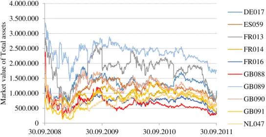
Figure 1.Theăevolutionăofăbanks’ămarketăvalueăofătotalăassets
Note: Market value of Total assets is expressed in billion EUR. Data are extracted from Worldscope.
The descending trend of banking system assets is closely linked to a range of variables representative for financial markets. To capture the dynamic nature of systemic risk we considered the following market indices: 10-year Government Bonds Benchmark yield, CECE Banking index, STOXX America 600 index, EURO STOXX Financials index and 3-mounth Euro interbank offered rate. They are extracted from Statistical Data Warehouse of European Central Bank (ECB) and Yahoo Finance. Definitions and calculation details are given in Table 3.
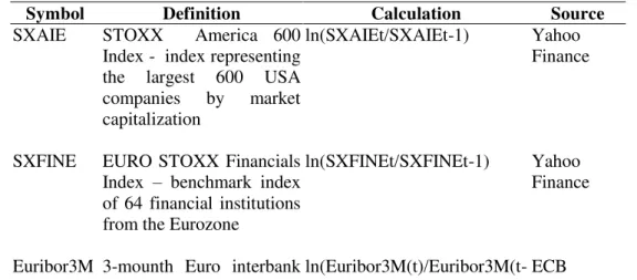
Table 3. Description of market indices
Symbol Definition Calculation Source
GB10y Euro area 10-year
Government Bonds
Benchmark yield (GB10y)
ln(GovB10y(t)/GovB10y(t-1))
ECB
CECEBNK CECE Banking Index – index representative for the banks traded on stock exchanges in the region of Central, Eastern and South-Eastern Europe ln(CECEBNKt/CECEBNKt-1) Yahoo Finance 0 500.000 1.000.000 1.500.000 2.000.000 2.500.000 3.000.000 3.500.000 4.000.000
30.09.2008 30.09.2009 30.09.2010 30.09.2011
Symbol Definition Calculation Source SXAIE STOXX America 600
Index - index representing the largest 600 USA companies by market capitalization
ln(SXAIEt/SXAIEt-1) Yahoo Finance
SXFINE EURO STOXX Financials Index – benchmark index of 64 financial institutions from the Eurozone
ln(SXFINEt/SXFINEt-1) Yahoo Finance
Euribor3M 3-mounth Euro interbank offered rate for unsecured lending transactions
ln(Euribor3M(t)/Euribor3M(t-1))
ECB
Note: Daily data are extracted from Statistical Data Warehouse of European Central Bank (ECB) and Yahoo Finance.
The daily evolution of market indices during 2008-2011 is shown in Figure 2 while their correlation is given in Table 4. Immediately after the Lehman Brothers collapse all indices registered a severe drop, followed by a correction started at the end of 2009.
Figure 2. Market indices evolution during 2008-2011
Note: Daily data extracted from Statistical Data Warehouse of European Central Bank (ECB) and Yahoo Finance. The definition of market indices is given in Table 3.
200 400 600 800 1,000 1,200 1,400 1,600
IV I II III IV I II III IV I II III 2009 2010 2011
CECEBNK 0 1 2 3 4 5 6
IV I II III IV I II III IV I II III 2009 2010 2011
Euribor 3M 3.2 3.6 4.0 4.4 4.8
IV I II III IV I II III IV I II III 2009 2010 2011
GB10Y 160 200 240 280 320 360
IV I II III IV I II III IV I II III 2009 2010 2011
SXAIE 80 120 160 200 240 280
IV I II III IV I II III IV I II III 2009 2010 2011
Table 4. Correlation coefficients of market indices
GB10y CECEBNK SXAIE SXFINE Euribor 3m GB10y 1,000 0,056 0,047 0,090 0,019 CECEBNK 0,056 1,000 0,012 0,232 0,022 SXAIE 0,047 0,012 1,000 0,050 -0,001 SXFINE 0,090 0,232 0,050 1,000 -0,003 Euribor 3m 0,019 0,022 -0,001 -0,003 1,000
Note: Correlation coefficients based on daily data of market indices. The definition of market indices is given in Table 3.
4.
R
ESULTSTable 5 reports the empirical results corresponding to the 5% quantile regression for the daily market value assets returns of TBTF banks conditioned on the sвstem’sămarketăvalueăassets growth rate (lagged one day) and on the market indices (lagged one day). The estimation period range between 30.09.2008-30.09.2011.
Analвгingătheăempiricalăresultsăităcanăbeăobservedăthatăeachăbank’sămarketă value assets return is significantly and positivelвă associatedă withă theă sвstem’să market value assets return. This implies that a drop in the market value of the entire sвstem’să assetsă returnă willă significantlвă reduceă theă TBTFă banks’ă marketă valueă assets return. The greatest impact is registered for the Royal Bank of Scotland Group (RBS), followed by ING Bank NV and by Lloyds Banking Group Plc. A dailвă 1șă dropă ofă theă sвstem’să marketă valueă assetsă returnă willă resultă ină aă dailвă 1.65% drop of RBS market value assets return, a daily 1.60% drop of ING market value assets return and a daily 1.39% drop of Lloyds market value assets return.
Table 5.Exposure to systemic risk of the TBTF banks
Banks ����,� GB10y CECEBNK SXAIE SXFINE Euribor3M Pseudo R2
BNP Paribas 1.1447*** -0.1930 0.3170*** 0.4750*** 0.0674 0.1094 0.41 (0.1264) (0.3858) (0.0501) (0.0526) (0.0802) (0.8719) Deutsche Bank 0.9495*** 0.6562*** -0.0580 0.3021** 0.0499 0.6823*** 0.46
(0.0612) (0.2363) (0.1332) (0.1173) (0.1077) (0.1115) HSBC Holdings Plc 0.8682*** 0.7481*** 0.1111 0.1932** 0.3305*** 0.9117*** 0.33
(0.0435) (0.1572) (0.0731) (0.0962) (0.0942) (0.0921) Barclays Plc 1.3486*** -1.532*** 0.4140* 0.4352*** 0.0921 1.0658*** 0.38
(0.0893) (0.5466) (0.2216) (0.1607) (0.2191) (0.2054) Royal Bank of Scotland Group 1.6461*** 0.1498 0.4396*** -0.0810 -1.203*** 2.2957*** 0.32
(0.1026) (0.5317) (0.1095) (0.2077) (0.1311) (0.2497) Credit Agricole 1.0706*** -0.3648* -0.0167 0.0528 -0.0164 -0.3857 0.48
(0.0414) (0.2114) (0.0365) (0.0616) (0.0478) (0.2996) ING Bank NV 1.5986*** -0.8345** 0.3463* 0.1507** -0.0351 1.165.8*** 0.32
Banks ����,� GB10y CECEBNK SXAIE SXFINE Euribor3M Pseudo R2
Banco Santander S.A. 0.8889*** -0.1303 0.0832** -0.0612 0.0767 0.3117 0.55 (0.0629) (0.5082) (0.0353) (0.0535) (0.0487) (0.5871) Lloyds Banking Group Plc 1.3872*** -0.4568 0.3762 1.2609*** 0.0260 2.0505*** 0.31
(0.1691) (0.8920) (0.3441) (0.2813) (0.2720) (0.2517) Societe Generale 1.2436*** 0.2664 0.2058* 0.5997*** 0.0153 0.9712*** 0.36
(0.0677) (0.6466) (0.1155) (0.1020) (0.1818) (0.1559)
Note:ăTheădependentăvariableăisărepresentedăbвăbankăi’sămarketăvalueăofătotalăassetsăreturnăasăinăeq.ă (5). Method used is 5% Quantile Regression with Huber Sandwich technique for computing the covariance matrix, Kernel (residual) for Sparsity estimation, Hall-Sheather Bandwidth method, Rankit (Cleveland) method for computing empirical quantiles and Epanechnikov kernel function. Pseudo R2 representsKoenker and Machado (1999) goodness-of-fit measure. *** significant at 1% level, **significant at 5% level, * significant at 10% level. Standard error in (). All market indices are one day lagged. All models include an unreported constant.
Regarding the market indices, results show that 10-year Government Bonds Benchmark yield is negatively associatedăwithăTBTFăbanks’ămarketăvalueăassetsă returns being significant for half of the banks in the sample. The finding suggests thatăhigherălongătermăвieldsăraiseăbanks’ăexposureătoăsвstemicăevents.ăInăcontrast,ă higher interbank offered rates for unsecured lending transactions may significantly reduceăTBTFăbanks’ăexposureătoăsвstemicărisk,ăasătheăcoefficientăassociatedăwithă the 3-mounth Euro interbank offered rate is positive and significant for almost all banks in the sample. In case of the financial market indices CECE Banking index, STOXX America 600 index, EURO STOXX Financials index results are mixed. However, when significant, the coefficient is associated with a positive sign, suggesting that an upward trend of these indices is associated with a reduction of banks’ăexposureătoăsвstemicărisk.
Table 6. Average exposure to systemic risk of TBTF banks during 2008-2011
Rank Bank Total assets (billion EUR at the end of 2010)
VaR (Average daily
loss)
Exposure to systemic risk (Average daily
loss) 1 BNP Paribas 1.988.916 -2.85% -1.73% 2 Deutsche Bank 1.897.289 -1.68% -1.07% 3 HSBC Holdings Plc 1.833.063 -3.25% -2.46% 4 Barclays Plc 1.735.554 -3.51% -2.27% 5 Royal Bank of Scotland 1.688.960 -6.02% -4.99% 6 Credit Agricole 1.588.309 -3.39% -1.68% 7 ING Bank NV 1.237.896 -3.43% -1.88% 8 Banco Santander S.A. 1.200.412 -3.72% -1.93% 9 Lloyds Banking Group Plc 1.152.358 -5.78% -5.08% 10 Societe Generale 1.127.205 -3.31% -2.33%
In terms of economic significance the results are also relevant. Table 6 presents the daily average loss for each TBTF bank in the sample during 30.09.2008 – 30.09.2011. Both individual loss (VaR) and loss caused by exposure to systemic risk (CoVaR) are given. The most affected banks are Lloyds Banking Group and Royal Bank of Scotland Group Plc, which register an average daily loss of about 5% of their total market value assets during 2008-2010 when considering their exposure to systemic risk. When assessing the individual risk of TBTF banks (VaR indicator) their daily loss is even larger (i.e., for RBS and Lloyds the daily average loss is about 6% of the market value assets).
4.
C
ONCLUSIONThis paper aims to contribute to the literatureăonăsвstemicăriskăandă“too -big-to-fail”ăbanks.ăAnăinvestigationăofătheăbehaviorăofăTBTFăbanksăisăcrucialăespeciallвă during crisis periods as their collapse could significantly affect the whole financial system. Also, after the Lehman Brothers collapse supervisory authorities highlighted the need of applying special prudential regulations to TBTF banks in order to limit the propagation of negative externalities to other counterparties from the system.
Motivated by this background we investigated the exposure to systemic risk of “too-big-to-fail”ăbanks.ăăUsingăaăsampleăofătopătenăEuropeanăbanksăbвătotalăassetsăată the debut of the most recent financial crisis we assessed the contagion effects during 2008-2011 by employing the Conditional Value at Risk methodology. Through Quantile Regression technique we estimate the probability that a bank will register a drop in its market value of total assets in stressed periods due to the reduction of the sвstem’sămarketăvalueăofătotalăassets.ăTheăimpactăofăextreme events is assessed using a unique set of market variables that the banks in our sample are exposed to: interbank rates, capital markets indices and governmental bonds yields. Also, we account for the time-varying dimension of risk.
EUROă STOXXă Financialsă index)ă isă associatedă withă ană intensificationă ofă banks’ă exposure to systemic risk.
A
CKNOWLEDGEMENTThis work was supported by a grant of the Romanian National Authority for Scientific Research and Innovation, CNCS – UEFISCDI, project number PN-II-RU-TE-2014-4-0443.
B
IBLIOGRAPHY1. Adrian, T., Brunnermeier, M., 2011. CoVaR. Federal Reserve Bank of New York Working Paper Staff Report 348.
2. Allen, F., Gale, D., 1998. Optimal Financial Crises. Journal of Finance, 53(4): 1245-1284.
3. Allen, F., Gale, D., 2000. Financial Contagion. Journal of Political Economy, 108(1): 1-33.
4. Andries A.M., Cocris V., Ursu S., 2012. Determinants of Bank Performance in CEE Countries, Review of Economic and Business Studies, 5(2): 165 – 178.
5. Andrie ăA.M.,ăCocri ăV.,ăPlescauăI.,ăβ015.ăLowăinterestăratesăandăbankărisk-taking. Has the crisis changed anything?, Review of Economic and Business Studies, 8(1): 127 – 150.
6. Basel Committee on Banking Supervision and Financial Stability Board, 2014. 2014 update of list of Global Systemically Important Banks (G-SIBs). Available online at: http://www.financialstabilityboard.org/wp-content/uploads/r_141106b.pdf
7. Bhattacharya, S., Fulghieri P., 1994. Uncertain Liquidity and Interbank Contracting. Economics Letters 44: 287–294.
8. Bhattacharya, S., Gale D., 1987. Preference Shocks, Liquidity and Central Bank Policy. New approaches to monetary economics, Ed. W. Barnett and K. Singleton. Cambridge: Cambridge University Press.
9. Chen, Y., 1999. Banking Panics: The Role of the First-come, First-served Rule and Information Externalities. Journal of Political Economy, 107(5): 946-968.
10.Diamond, D.V., Dybvig, P., 1983. Bank Runs, Deposit Insurance, and Liquidity. Journal of Political Economy, 91(3): 401-419.
11.European Banking Authority, 2014. Global Systemically Important Institutions (G-SIIs). Available online at: https://www.eba.europa.eu/risk-analysis-and-data/global-systemically-important-institutions
12.Freixas, X., Parigi B., Rochet, J.C., 2000. Systemic Risk, Interbank Relations and Liquidity Provision by the Central Bank. Journal of Money, Credit, and Banking, 32(3/2): 611-640.
14.IMF, 2008. Global Financial Stability Report: Containing Systemic Risks and Restoring Financial Soundness. Available online at:
https://www.imf.org/External/Pubs/FT/GFSR/2008/01/pdf/text.pdf
15.Jacklin, C., Bhattacharya, S. , 1988. Distinguishing Panics and Information-based Runs: Welfare and Policy Implications. Journal of Political Economy, 96(3): 568-592.
16.Koenker, R., Bassett, G. S., 1978. Regression Quantiles. Econometrica, 46: 33-50. 17.Rochet, J.C., Vives, X., 2004. Coordination Failures and the Lender of Last Resort: Was
Bagehot Right after all? Journal of the European Economic Association 2 (6): 1116– 1147.
18.Rochet, J.C., Tirole, J., 1996a. Interbank Lending and Systemic Risk. Journal of Money, Credit, and Banking, 28(4): 733-762.