Model Predictive Approach to Precision Contouring Control for Feed Drive Systems

Journal of Computer Science 6 (8): 844-851, 2010 ISSN 1549-3636

© 2010 Science Publications

Corresponding Author: A. El Khalick M., Department of Mechanical Engineering, Toyohashi University of Technology, 1-1 Hibarigaoka, Tempaku-cho, Toyohashi, Aichi 441-8580, Japan Tel: +81-90-9911-0445

Model Predictive Approach to Precision Contouring Control for Feed Drive Systems

A. El Khalick M. and N. Uchyiama

Department of Mechanical Engineering, Toyohashi University of Technology,

1-1 Hibarigaoka, Tempaku-cho, Toyohashi, Aichi 441-8580, Japan

Abstract: Problem statement: High precision machining requires high capability of multi-axis feed drive systems to follow specified contour accurately. Although each feed drive axis is controlled independently in many industrial applications such as X-Y tables and Computer Numerical Control (CNC) machines, machining precision is evaluated by error components orthogonal to desired contour curve. Contouring controller design is required for precision machining, which should consider disturbance and dynamics variation such as friction, cutting force and workpiece mass change. Approach: This study applied model predictive design to contouring control systems. Model predictive control utilized an explicit process model and tracking error dynamics to predict the future behavior of a plant and hence it is effective for precision machining in machine tool feed drives. To improve the contouring performance, a new performance index was proposed in which error components orthogonal to the desired contour curve are more important than tracking errors with respect to each feed drive axis. Controller parameters were calculated in real time by solving an optimization problem. Results: The proposed controller was evaluated by computer simulation for circular and non-circular trajectories. Weighting factors of performance index terms were used as tuning factors of the proposed controller. Simulation results showed that a better contouring performance can be obtained by choosing of the weighting factors in performance index items appropriately. Conclusion/Recommendations: A model predictive contouring controller for biaxial feed drive systems was presented. Simulation results demonstrated that the proposed approach can significantly improve the contouring accuracy.

Key words: Contouring control, model predictive control, feed drive systems INTRODUCTION

The ultimate goal in many industrial applications such as X-Y tables, Computer Numerical Control (CNC) machines and industrial manipulators is to reduce the contouring error as much as possible to keep high precision motion. Two main control approaches are used to improve the contouring performance, tracking control approach and contouring control approach. In tracking control approach, the dedicated control law of each drive control loop tries to minimize the tracking error independent of other control loops. In addition, any disturbance in one control loop is corrected only by this loop. The other control loops will not receive any information about that disturbance and it will run as if the disturbed control loop is functioning normally. On the other hand, the contour errors to the desired path are evaluated in real time and these errors are eliminated via feedback control in contouring control systems. To improve the tracking accuracy in

and Tomizuka (2001) proposed the Task Coordinate Frame (TCF) and Lo and Chung (1999) proposed the Tangential Contouring Controller (TCC) for biaxial motion, The proposed controller is based on a coordinate transformation between the X-Y frame and a Tangential-Contouring (T-C) frame defined along the contour. Cheng and Lee (2005) proposed a real-time contour error estimation algorithm. Ye et al. (2002) proposed a new Cross-Coupled Path Precompensation (CCPP) algorithm for a Rapid Prototyping and Manufacturing (RPM) systems. To reduce the contour error by optimization of controller parameters using a genetic algorithm, Tarng et al. (1999) presented a cross-coupled fuzzy federate control scheme.

Predictive control refers to a class of model based controllers that utilizes an explicit process model to predict the future response of a plant. Boucher et al. (1990) proposed using Generalized Predictive Control (GPC), which incorporates both reference preview action, as well as disturbance rejection into the same control scheme. This formulation is also extendable to include control law and tracking error constraints. Zhe and Chen (2001) proposed a cross-coupled generalized predictive control algorithm. This provides a combined feedback-feed forward controller resulting in zero-pole cancelation of poles that do not correspond to the reference models. They presented a new cost function in which synchronization errors are embedded. Susanu and Dumur (2005) proposed a hierarchical predictive control architecture dedicated to axis feed drives of machining centers. The considered performance index is a weighted sum of predicted tracking errors from a minimum prediction horizon N1 to a maximum horizon N2 and future control signal increments over the control horizon, nevertheless motion control based only on the tracking ability of each axis in multi feed drive system does not always guarantee high precision machining.

To improve the contouring performance in machine tool feed drive systems, this study presents a model predictive contouring controller design based on coordinate transformation approach. The main advantage of the proposed approach is to provide easy adjustment of controller parameters by including transformed error and input signals in the performance index of model predictive control. The control law has been analytically derived by real time optimization of the performance index so that the resulting control system provides improved performance in terms of tracking and contouring errors. In addition, the proposed approach takes into account the dynamics modeling errors, cutting forces and disturbances such as friction.

MATERIALS AND METHODS

Contouring error definition: Contouring error is defined as the shortest distance between the actual contour and the desired one. The relation between the contouring error and the tracking error in each feed drive axis is shown in Fig. 1. Two coordinate frames are used, Σw, whose axes X and Y correspond to feed-derive axes and it is fixed frame. The curve c is the desired contour curve of the point of a machined part driven by the feed drive system. The desired position of the point of the machined part at time t and defined in

Σw is r = [r1, r2]T. The actual position of the feed drive system is represented by x = [x1, x2]T which also is defined in the fixed frame. The second coordinate frame Σl is attached at r and its axes are l1 and l2. The axis l1 is in the tangential direction of c at r and the direction of l2 is perpendicular to l1. The tracking error in each feed drive axis is defined as follows:

T w x y

e =[e e ] = −r x. (1)

This error can be expressed with respect to Σl as follows:

T T

l t n w

e [e e ] R e ,

cos sin

R

sin cos

= =

θ − θ

 

= _{θ θ}

 

(2)

where, θ is the inclination of Σl-Σw. Since it is difficult to calculate the actual contouring error in real time for complex contour, the error component en is only an approximate value of the contouring error ec, which is the distance between the actual position x and the nearest point on the desired curve c.

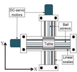
Fig. 2: Typical biaxial feed drive system

Modeling of biaxial feed drive system: A typical biaxial feed drive system as shown in Fig. 2 is used to demonstrate the improvement in the contour accuracy by the proposed control system. Two DC servo motors are used to drive the feed drive system, which are commonly used in industrial applications. Feed drive system is generally represented by the following decoupled second-order system:

i i T x y

Mx Cx f ,

M diag{m },

C diag{c },i x, y,

f [f f ] .

+ = = = = = ɺɺ ɺ (3)

where, mi(>0), ci(≥0) and fi are the table mass, viscous friction coefficient and driving force on the drive axis i, respectively. The symbol diag{ai} denotes a diagonal matrix with the elements ai at the ith diagonal positions. Two ball screws are used to convert angular motion of the motors to linear motions of the table. The motor dynamics for driving the feed drive system are described as follows:

}

{

}

{

{

}

mi mi T mi m1 m 2

i i

i

T T

x y x y

N Z Kv,

[ , ] ,

N diag n , Z diag z ,

K diag k , i x , y

[ , ] , v [v , v ] ,

θ + θ + τ= θ = θ θ

= =

= =

τ= τ τ =

ɺɺ ɺ

(4)

where, θmi, ni(>0), zi(≥0), ki(>0), τi and νi are the rotational angle of the motor, motor inertia, viscous friction coefficient, torque-voltage conversion ratio, torque for driving the feed drive system and the input

voltage to the motor of the ith drive axis respectively. Relations among force fi torque τi, position xi and angle

θmi are represented as follows:

i i mi

i i

i

2 p

f , x

p 2

πτ θ

= =

π (5)

where, pi is the pitch of the ball screw.

Model predictive control: A discrete time model describes the plant dynamics has been used to estimate the output of the plant. The following transfer function model is used to describe the biaxial feed drive system:

d 1 1

i i

i 1 i 1 i

i i

1

i i

q B (q ) C (q )

y (k) u (k 1) e (k),

A (q ) T (q )

e (k) (k), 1 q

− − −

− −

−

= − +

=∆ζ ∆ = −

(6)

where the index i (i = x, y) denotes the corresponding motion axis of the biaxial feed drive system, k is the normalized discrete time, yi(k) and ui(k) are the output and the control input of each feed drive axis respectively, d is the time delay in the process samples, ζi(k) represents a random disturbance and Ai(q−1), Bi(q−1), Ci(q−1) and Ti(q−1) are polynomials for the ith feed drive axes in the delay operatorq−1. The predicted output of the plant is as follows:

ˆd 1

i i

i 1 i i i

i i

ˆ

q B (q ) F

ˆ ˆ

y (k i) u (k i 1) [y (k) y (k)]

ˆ ˆ

A (q ) C

− − −

+ = + − + − (7)

The symbol ^ denotes estimates, Fi is a polynomial that satisfies the following Diophantine equation: 1 i i i i i C F E q T T −

= + (8)

The purpose of this controller is for the feed drive to follow the reference trajectory as closely as possible and the following performance index has been presented (Soeterboek, 1992):

( )

( )

* T T

i i i i i i i i T

i i i m i i P

T

i i i m i i P

T

i i i P i

n i

i i

di

ˆ ˆ

J (y w ) (y w ) u u ,

ˆ ˆ ˆ

y [P y (k H ) ,..., P y (k H )] ,

w [P 1 w (k H ),..., P 1 w (k H )] ,

ˆ

u [u (k),..., u (k H d 1)] ,

Q

u (k) u (k).

Q ∗ ∗ ∗ ∗ ∗ ∗ ∗ ∗ ∗ ∗ ∗

= − − + ρ

= + +

= + +

= + − −

=

Where:

Pi = A polynomial used to tune the servo behavior of the control system

HmandHp = The minimum cost horizon and prediction horizon respectively

wi = The reference signal

ρi = A non-negative weighting factor to adjust the control input

Qniand Qdi = Monic polynomials with no common factors and can be used to obtain the weighting factor for ui(k)

Model predictive contouring controller: In the previous performance index (9) as well as (Susanu and Dumur, 2005), only the tracking errors with respect to each feed drive axis are included. The error components orthogonal to the desired contour curves are more important than tracking errors and hence the orthogonal error component is included in the proposed performance index with control inputs in the normal and tangential directions as follows:

p p p p

j j j j

m m m m

j j j

H H H H

2 2 2 2

cn n ct t n n t t

j H j H j H j H

T T T

t j n x y

J e e u u

[u u ] R [u u ]

= = = =

=ρ +ρ +ρ +ρ

=

∑

∑

∑

∑

(10)

Where:

ρcn and ρct = Weighting factors to adjust the importance of the error component in the orthogonal and tangential directions, respectively

ρn and ρt = Weighting factors used to adjust the control inputs in the normal and tangential directions, respectively

uxj, uyj, unj and utj = The jth control inputs in X, Y, N and T directions, respectively

Minimization of the performance index (10) gives:

1 xj xx xy xx yj yx yy yy

u Π Π Γ

u Π Π Γ

−

     

=

     

      (11)

T 2 2 T 2 2 T

xx cn ct x x n t

T T T

xy ct cn x y t n

T T T

yx ct cn y x t n

T 2 2 T 2 2 T

yy cn ct y y n t

Π M [( S C )G G ( S C )Φ Φ]M

Π M SC[( )G G ( )Φ Φ]M

Π M SC[( )G G ( )Φ Φ]M

Π M [( C S )G G ( C S )Φ Φ]M

= ρ + ρ + ρ + ρ

= ρ − ρ + ρ − ρ

= ρ − ρ + ρ − ρ

= ρ + ρ + ρ + ρ

(12)

T T 2 2

xx n t x x

t n y y

2 2 *

x cn ct x x x x x x x ct cn y y

* y y y y y

T T 2 2

yy n t y y

t n x x

y

Γ M [Φ (( S C )( u ΦNu )

SC( )( u ΦNu ))

G (( S C )(H u F c ζ G Nu x )

SC( )(H u

F c ζ G Nu y ))]

Γ M [Φ (( C S )( u ΦNu )

SC( )( u ΦNu ))

G ((

= − ρ + ρ +

+ ρ − ρ +

+ ρ + ρ + + + −

+ ρ − ρ

+ + + −

= − ρ + ρ +

+ ρ − ρ +

+ ⌣ ɶ ⌣ ɶ ⌢ ⌣ ⌢ ⌣ ⌣ ɶ ⌣ ɶ

2 2 *

cn ct y y y y y y y ct cn x x

* x x x x x

C S )(H u F c ζ G Nu y )

SC( )(H u

F c ζ G Nu x ))]

ρ + ρ + + + −

+ ρ − ρ

+ + + − ⌢ ⌣ ⌢ ⌣ (13) Where:

x and y = Refer to the corresponding feed drive axis M and N = Matrices that consist of plant parameters

with dimensions HP− ×dˆi Hc and

i

P ˆi P C

H − ×d nΦ+n −H respectively

Hc = The control horizon:

H

G

H

G

1,0 1, n

1, n 1,0

j,0 j, n

j,n j,0

1 0 0

0 1

0 0

0 0

0

M , N

h h

0 0 1

0 0 g g

h h

0 0 g g

      _{ }   _{ }   _{ }   _{ }   _{ } =_{ } =     _{ }   _{ }   _{ }           ⋯ ⋯ ⋮ ⋮ ⋮ ⋮ ⋱ ⋱ ⋱ ⋯ ⋯ ⋯ ⋮ ⋮ ⋯ ⋯ ⋯ ⋮ ⋮ ⋮ ⋮ ⋯ ⋯ (14)

where, j = HP−Hc−dˆ . Gi, Hi and Fi are matrices as

follows: P P P ˆ i(d 1) i0 i1 i0

i i ij

ˆ i0

i(H d 1)

iH ˆ i(d 1) i ij iH H

g 0 0

g g

G , H H ,

0 g g H F F F F + − − +               =_{ } =_{ }                       =_{ }         ⋯ ⋮ ⋱ ⋮ ⋮ ⋱ ⋮ … … ⋮ ⋮ (15)

ˆ im d

i im

im P

i i

ˆ

B H _ˆ

G q , m [d 1,..., H ]

ˆ ˆ

A A

− +

= + = + (16)

j im

im P

i i

1 F _ˆ

E q , m [d 1,..., H ]

ˆ ˆ

A A

−

= + = + (17)

Φ = A lower triangular matrix of dimension

P ˆi P ˆi

(H −d ) (H× −d )

Ω = A matrix of dimension (HP−d )ˆi ×nΩ, with

nΩ = max (nQni, nQdi)

Φ andΩ = Consist of the elements of the polynomials Φ and Ω respectively which satisfy the following Diophantine equation:

1 ni

di di

Q

q

Q Q

− Ω

= Φ + (18)

x*andy*are as follows:

( )

( )

( )

( )

x m x P

y m y P

x [P 1 x(k H ),..., P 1 x(k H )]

y [P 1 y(k H ),..., P 1 y(k H )]

∗ ∗

= + +

= + + (19)

where, x and y are the reference trajectories in X and Y directions respectively and uɶ_,u⌣_,u⌢_{and c are given}

by:

i

T

di di

T

c P

i

T i i

i

u(k 1) u(k n )

u [ ,..., ] ,

Q Q

u [u(k 1),..., u(k H n n )] ,

u(k)

u ,

ˆ A

ˆ

y (k) y (k)

c [c(k), c(k 1)...] ,c(k)

T

Ω

Φ

− −

=

= − + − −

=

−

= − =

ɶ

⌣

⌢ (20)

RESULTS

To verify the effectiveness of the proposed controller, computer simulation has been conducted for circular and non-circular reference trajectories. The parameters of the feed drive system are shown in Table 1. The biaxial feed drive system is represented in discrete time by the following polynomials:

1 1 2

i

1 1 2

i

A (q ) 1 -1.97q 0.97q

B (q ) 0.28e-6q 0.28e-6q

− − −

− − −

= +

= + (21)

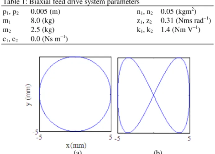
Table 1: Biaxial feed drive system parameters

p1, p2 0.005 (m) n1, n2 0.05 (kgm2)

m1 8.0 (kg) z1, z2 0.31 (Nms rad−1)

m2 2.5 (kg) k1, k2 1.4 (Nm V−1)

c1, c2 0.0 (Ns m−1)

(a) (b)

Fig. 3: Reference trajectories. (a) Circular and (b) non-circular

This model is obtained from continuous-time model by using zero-order hold and sampling time T = 0.005 sec.

Two reference trajectories are used to simulate the proposed controller as follows:

• Circular reference trajectory

x 5sin ( t) (mm)

10

y 5cos ( t) (mm)

10

π =

π =

(22)

• Non-circular reference trajectory

x 5sin ( t) (mm)

10

x 5sin ( t) (mm)

5

π =

π =

(23)

Circular and non-circular reference trajectories are shown in Fig. 3a and b respectively.

For the circular reference trajectory the actual contouring error can be easily calculated by the following equation, although this equation is used for verification only and not used to calculate the controller parameters:

2 2 c

e = −5 x +y (mm) (24)

(a) (b)

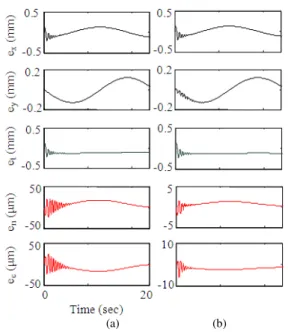
Fig. 4:Simulation results (circular trajectory). (a) ρcn =1; (b) ρcn =10

(a) (b)

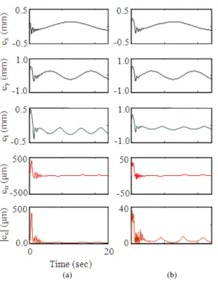
Fig. 5: Simulation results (non-circular trajectory). (a)

ρcn = 1; (b) ρcn = 10

Simulation results for circular reference trajectory, where the weighting factor for error components orthogonal to the desired contour curve ρcn is set to one, are shown in Fig. 4a. Since the error components orthogonal to the desired contour curves are more important than tracking errors with respect to each feed drive axis, a better contouring performance is obtained by increasing the weighting factor for error components orthogonal to the desired contour curve. Figure 4b shows the simulation results for circular trajectory case with ρcn = 10.

(a) (b)

Fig. 6: Simulation results (circular trajectory). (a)

ρt = ρn; (b) ρt = 103ρn

To verify the effectiveness of the proposed controller to follow non-circular trajectories effectively, the non-circular trajectory is used. For the non-circular trajectory, a minimization problem is solved offline to calculate the magnitude of the actual contouring error at time tkas follows:

{

} {

}

c k _t 1 k 1 2 k 2

e (t ) =min x (t )−r (t) + x (t )−r (t) mm (25)

Note that this error magnitude is used only for verification purpose. The Simulation results for the non-circular trajectory, where the weighting factor for error components orthogonal to the desired contour curve is set to values same as those used in Fig. 4, are shown in Fig. 5a and b.

Figure 6a shows the simulation results for circular reference trajectory, where equaled weighting factors are used to adjust the control inputs in the orthogonal and tangential directions. The improved results for contouring error are obtained in Fig. 6b by adjusting the control input weighting factor in the orthogonal direction to be thousand times less than that in the tangential direction.

(a) (b)

Fig. 7:Simulation results (non-circular trajectory). (a)

ρt = ρn; (b) ρt = 103ρn

DISCUSSION

The error components orthogonal to the desired contour curves are more important than tracking errors with respect to each feed drive axis and hence by increasing the weight factor for the orthogonal error components in the performance index gives a reasonable enhancement of the contouring performance. In addition, control inputs in the orthogonal and tangential direction are important tuning parameters for the proposed contouring controller by which the control energy can be adjusted to be smaller in the tangential direction than that in the orthogonal direction.

CONCLUSION

A model predictive contouring controller for biaxial feed drive systems based on coordinates transformation has been presented. To verify the effectiveness of the proposed control approach, computer simulation has been conducted for circular and non-circular reference trajectories. Simulation results show that the proposed controller can significantly improve the contouring accuracy for any smooth contour. Applying this approach to three or five axis machine are left for future study.

ACKNOWLEDGMENT

This research was supported by KAKENHI21560119. The authors would like to express grateful thanks for this support.

REFERENCES

Boucher, P., D. Dumur and K.F. Rahmani, 1990. Generalized predictive cascade control for machine tools drives. Ann. CIRP., 39: 357-360. DOI: 10.1016/S0007-8506(07)61072-5

Cheng, M.Y. and C.C. Lee, 2005. On real-time contour error estimation for contour following tasks. Proceeding of the IEEE/ASME International Conference of Advanced Intelligent Mechatronics, July 2005, Monterey, CA., pp: 1047-1052. DOI: 10.1109/AIM.2005.1511148

Chiu, G.T.C. and M. Tomizuka, 2001. Contouring control of machine tool feed drive systems: A task coordinate frame approach. IEEE Trans. Control Syst. Technol., 9: 130-139. DOI: 10.1109/87.896754

Ho, H.C., Y.J. Yush and S.S. Lu, 1990. A decoupled path-following control algorithm based upon the decomposed trajectory error. Int. J. Mach. Tools Manufact., 39: 1619-1630. DOI: 10.1016/S0890-6955(98)00095-9

Koren, Y., 1980. Cross-coupled biaxial computer controls for manufacturing systems. ASME J. Dyn. Syst., Measure., Control, 102: 265-272. DOI: 10.1115/1.3149612

Lo, C.C. and C.Y. Chung, 1999. Tangential-contouring controller for biaxial motion control. ASME. J. Dyn. Syst., Measure., Control, 121: 126-129. DOI: 10.1115/1.2802430

Masory, O., 1986. Improving contouring accuracy of NC/CNC systems with additional velocity feed forward loop. ASME J. Eng. Ind., 108: 227-230. DOI: 10.1115/1.3187068

Soeterboek, R., 1992. Predictive Control a Unified Approach. 1st Edn., Prentice Hall International Limited, UK., ISBN: 0136783503, pp: 300. Susanu, M. and D. Dumur, 2005. Using predictive

techniques within CNC machine tools feed drives. Proceeding of the IEEE Conference on Decision and Control, Dec. 12-15, IEEE Computer Society, USA., pp: 5150-5155.

Tomizuka, M.J., 1987. Zero phase error tracking algorithm for digital control. ASME J. Dyn. Syst. Measure. Control, 109: 65-68. DOI: 10.1115/1.3143822

Ye, X., X. Chen, X. Li and S. Huang, 2002. A cross-coupled path precompensation algorithm for rapid prototyping and manufacturing. Int. J. Adv. Manufact. Technol., 20: 39-43. DOI: 10.1007/s001700200121