www.atmos-chem-phys.net/9/1419/2009/ © Author(s) 2009. This work is distributed under the Creative Commons Attribution 3.0 License.
Chemistry
and Physics
Physical interpretation of the spectral radiative signature in the
transition zone between cloud-free and cloudy regions
J. C. Chiu1, A. Marshak2, Y. Knyazikhin3, P. Pilewski4, and W. J. Wiscombe2,5 1University of Maryland Baltimore County, Baltimore, MD, USA
2NASA/Goddard Space Flight Center, Greenbelt, MD, USA 3Boston University, Boston, MA, USA
4University of Colorado at Boulder, Boulder, CO, USA 5Brookhaven National Laboratory, New York, NY, USA
Received: 29 July 2008 – Published in Atmos. Chem. Phys. Discuss.: 26 September 2008 Revised: 26 January 2009 – Accepted: 26 January 2009 – Published: 23 February 2009
Abstract. One-second-resolution zenith radiance measure-ments from the Atmospheric Radiation Measurement pro-gram’s new shortwave spectrometer (SWS) provide a unique opportunity to analyze the transition zone between cloudy and cloud-free air, which has considerable bearing on the aerosol indirect effect. In the transition zone, we find a re-markable linear relationship between the sum and difference of radiances at 870 and 1640 nm wavelengths. The intercept of the relationship is determined primarily by aerosol prop-erties, and the slope by cloud properties. We then show that this linearity can be predicted from simple theoretical con-siderations and furthermore that it supports the hypothesis of inhomogeneous mixing, whereby optical depth increases as a cloud is approached but the effective drop size remains un-changed.
1 Introduction
The aerosol indirect effect is the largest source of uncertainty in the radiative forcing of climate (The Intergovernmental Panel on Climate Change, IPCC, Fourth Assessment Report, 2007). Using 11 GCM models, Stephens (2002) also showed the importance of cloud feedbacks in modeling responses of climate to a doubling of carbon dioxide. We cannot evaluate performance of climate models without accurate knowledge of aerosol forcing and cloud feedbacks (Diner et al., 2004).
Studies on aerosol direct and indirect effects demand a precise separation of cloud-free and cloudy areas (Charl-son et al., 2007; Koren et al., 2007). However, separation between cloud-free and cloudy areas from remotely sensed
Correspondence to:J. C. Chiu ([email protected])
measurements is ambiguous. From the ground, separations have been made using broadband pyranometer, microwave radiometer, total sky imager, radar, lidar, and ceilometer data (Long and Ackerman, 2000; Berendes et al., 2004; Long et al., 2006a, b; Taylor et al., 2008). Each instrument has a different field of view, sensitivity, and sampling resolution; in addition, each method uses different thresholds for the separation. From satellites, the separation depends on spa-tial resolution, illumination and observation geometry, sur-face types, and screening algorithms (Ackerman et al., 1998; Martins et al., 2002; Brennan et al., 2005; Gomez-Chova et al., 2007). While a separation is not free of ambiguity at any scale (Koren et al., 2008), it is important to understand the transition zone between cloud-free and cloudy areas.
Yet it has been difficult to study the transition zone using conventional data. Both satellite and in situ aircraft data are inadequate. Satellite data are hampered both by lack of high enough spatial resolution and by ambiguity in interpreting radiances due to 3-D radiative transfer effects. As a result, aerosol retrievals in the vicinity of clouds may be contami-nated by undetected clouds (Zhang et al., 2005) as well as by radiation reflected from clouds (Marshak et al., 2008). In addition, cloud properties in the collection 5 Moderate Reso-lution Imaging Spectroradiometer (MODIS) product are not reported for cloudy pixels that border clear-sky pixels, be-cause those cloudy pixels may include both clear and cloudy areas, and the retrievals of their microphysical properties are not reliable (Coakley et al., 2005).
On the other hand, in situ data are hampered by lack of fast enough time resolution. For measuring cloud microphysi-cal properties, most probes have no better than 1 to 10 Hz sampling rate, though some probes can sample faster (e.g., 2000 Hz from Gerber probes, Davis et al., 1999; and 1000 Hz from Fast Forward Scattering Spectrometer probe, Brenguier et al., 1998). However, due to tiny sample volumes, averag-ing over longer time periods is usually necessary to achieve statistical significance. If measurements are averaged to 1– 2 Hz with an aircraft speed of 100 m/s, the spatial resolution will be 50–100 m, which is not fine enough to study physical processes around cloud edges.
In situ data are also hampered by noise in measurements. For example, standard hot-wire liquid water probes are noisy at the 0.2 g m−3 level. Uncertainty of cloud microphysical measurements is in an order of 20% (Allan et al., 2008). The variations in the transition zone would be masked by such large noise values.
This paper aims to study changes of aerosol and cloud properties in the transition zone from radiative signatures measured by the new Atmospheric Radiation Measurement (ARM) Program shortwave spectrometer (SWS). The SWS is the first ground-based instrument that measures zenith ra-diances with high temporal (1-s) and spectral resolution in the visible and near-infrared region. Spectra from SWS con-tain rich information on radiative properties of aerosols and clouds to advance our understanding of physical processes in the transition zone, such as activation and evaporation of cloud droplets and humidification of aerosols.
2 Shortwave spectrometer and ancillary ARM data
The SWS, a ground-based instrument based upon the design of the airborne Solar Spectral Flux Radiometer (Pilewskie et al., 2003), was first deployed in March 2006 at the ARM Ok-lahoma site. The SWS measures zenith radiance at 418 wave-lengths between 350 and 2170 nm. The spectral resolution for visible and near infrared regions is 8 and 12 nm, respec-tively. The field of view is 1.4◦. The integration time of each
1-s measurement is about 300 ms. The SWS is calibrated
bi-weekly using the on-site ARM 12′′ integrating sphere that
is in turn calibrated by the 30′′ sphere at the NASA Ames
Research Center. Therefore, the absolute accuracy of mea-surements depends on the accuracy of the transfer standard from the 30′′sphere to the 12′′ sphere. The 30′′ sphere has an accuracy of 1–2%.
We used two discrete SWS wavelengths of 870 and 1640 nm to explore their spectral changes in more details. We selected these wavelengths to minimize Rayleigh scattering and maximize the sensitivity of zenith radiance to cloud opti-cal depth and cloud drop size. Neither liquid water nor vapor absorb sunlight at 870 nm wavelength. On the other hand, liquid water absorbs weakly at 1640 nm (and is amplified by multiple scattering within cloud), where there is negligible absorption by water vapor and carbon dioxide. We further normalized zenith radiance measurementIm,λat wavelength λusing:
Iλ=
π·Im,λ µ0·FTOA,λ
, (1)
whereIλ is the normalized zenith radiance; FTOA,λ is the solar irradiance at the top of the atmosphere; andµ0is the cosine of solar zenith angle (SZA). We denote normalized zenith radiances at 870 and 1640 nm hereafter as I870 and I1640, respectively, as well as
SUM =I870+I1640 (2a)
DIF =I870−I1640 (2b)
which are in many cases more informative and illustrative than radiances themselves.
We also used ancillary instruments and products to better understand atmospheric state and cloud field for case study. First, the ARM Total Sky Imager (TSI) captures cloud field images at a 30-s sampling interval with a half-hemispheric field of view (Long et al., 2001). A shadowband on the mirror blocks the intense direct-normal light from the sun. Although clouds of interest are those at the center of TSI images and are often blocked by the shadowband, one can see cloud evolution and movement from time series of cloud images. Second, cloud boundary heights were obtained at a 10-s resolution from the ARM Active Remotely Sensed Clouds Locations (ARSCL) product, based on measurements of cloud radar, micropulse lidar, and ceilometer (Clothiaux et al., 2000). Third, liquid water path was retrieved from ARM microwave radiometer measurements at a 20-s resolu-tion (Turner et al., 2007). Finally, wind speed was estimated from the merged sounding product (Miller et al., 2003). Note that the temporal resolutions of all ancillary data (10, 20, 30-s, and 1-min) are much lower than that of the SWS (1-s).
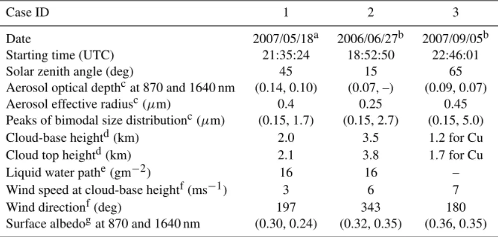
Table 1.Case summary.
Case ID 1 2 3
Date 2007/05/18a 2006/06/27b 2007/09/05b Starting time (UTC) 21:35:24 18:52:50 22:46:01
Solar zenith angle (deg) 45 15 65
Aerosol optical depthcat 870 and 1640 nm (0.14, 0.10) (0.07, –) (0.09, 0.07) Aerosol effective radiusc(µm) 0.4 0.25 0.45 Peaks of bimodal size distributionc(µm) (0.15, 1.7) (0.15, 2.7) (0.15, 5.0) Cloud-base heightd(km) 2.0 3.5 1.2 for Cu Cloud top heightd(km) 2.1 3.8 1.7 for Cu
Liquid water pathe(gm−2) 16 16 –
Wind speed at cloud-base heightf(ms−1) 3 6 7
Wind directionf(deg) 197 343 180
Surface albedogat 870 and 1640 nm (0.30, 0.24) (0.32, 0.35) (0.36, 0.35)
aData length is 300 s bData length is 120 s
cestimated from NASA’s Aerosol Robotic Network (AERONET)
destimated from ARM’s Active Remotely Sensed Clouds Locations (ARSCL) product eestimated from an ARM PI product (MWRRET)
festimated from ARM’s Merged Sounding product
gestimated from NASA’s Moderate Resolution Imaging Spectroradiometer (MODIS)
Note that aerosol properties at 1640 nm are not available at the Oklahoma site until May 2007.
is vegetated. For a single leaf, the reflectance at 870 nm is generally 1.2–1.5 times greater than that at 1640 nm (Walter-Shea and Norman, 1991). However, surface albedo depends not only on properties of single leaf, but also on canopy struc-tures (Knyazikhin et al., 1997). In this paper, values of sur-face albedo were based on MODIS collection 5 retrievals at a 500 m resolution (Schaaf et al., 2002).
3 Observed spectral signatures from SWS in the transi-tion zone
We chose three cases (Table 1) to show how the spectral signature of the transition zone changes between cloud-free and cloudy areas for different solar zenith angles. We made our choices using the following criteria. First, we sepa-rated cloudy from cloud-free times in the SWS data using radiances at wavelengths of 673 and 870 nm. Marshak et al. (2004) suggested that over a vegetated surface, a larger radiance at 673 nm than at 870 nm indicates a cloud-free sit-uation. For cloudy situations, the situation reverses; the ra-diance at 870 nm becomes larger. Second, we limited our-selves to cases in which the cloud-free and cloudy periods both lasted at least one minute, to avoid very small clouds and gaps. This criterion leads to 300–500 m sizes of cloud and gap, typical for fair weather cumulus (Joseph and Caha-lan, 1990; Lane et al., 2002). Third, to avoid messy situations in which the cloud itself is very fragmented, we excluded
cases in which the ratio of radiances at 673 nm and 870 nm changed by more than 10% during cloudy periods.
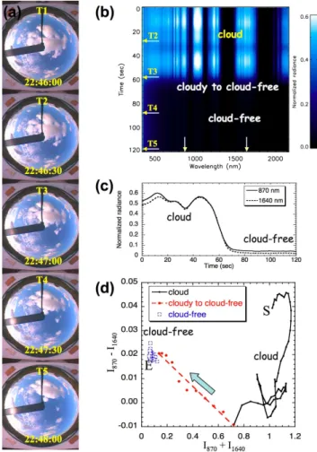
3.1 Case 1
Case 1 is a single small cumulus cloud passing over; we look at the transitions at both the beginning and end of the pas-sage. Images of the sky dome, taken by the TSI, are shown in Fig. 1a. The cumulus cloud of interest was blocked by the shadowband at 21:35 UTC, but could be seen in TSI im-ages after 21:36 UTC. The cloud moved toward the northeast (upper-right corner of the sky images) with a 3 m s−1speed at its cloud-base height of 2 km. Liquid water path of the cloud was∼16 g m−2. The sun was in the west with a solar zenith angle of 45◦. Because the sun was shining behind the cloud,
the radiometer was on the cloud’s shadowed side before the cloud passed over, and the illuminated side after.
Figure 1b shows the time series of Case 1 SWS spectral radiances as a color contour plot. The structure of this plot will be similar for the other two cases, so we describe it here briefly. The times (T1, etc.) indicated correspond to the images in Fig. 1a. The brighter colors indicate the cloudy period, the darker colors the cloud-free period, and the in-termediate colors the transition period, which obviously has a finite temporal (and hence horizontal) extent. The vertical black bands during the cloudy period are absorption bands of water vapor.
Fig. 1.Case 1, 18 May 2007 with a SZA of 45◦:(a)total sky im-ages (from TSI instrument), and(b)time-wavelength contour plot of SWS spectra measured from 21:35:24 to 21:40:24 UTC (300 s). SWS-observed zenith radiances have been normalized by the ex-traterrestrial solar spectrum and by cos(SZA). In (b), arrows pointed at the time axis correspond to the times of the sky images shown in (a), while arrows pointed at the wavelength axis correspond to 870 and 1640 nm. We also see strong water vapor absorption bands at wavelengths of 930, 1120, 1400, and 1900 nm. (c)is time series of radiances at 870 and 1640 nm corresponding to two slices of (b).
(d)is the plot of normalized radiance difference versus sum at wave-lengths of 870 and 1640 nm. Letters S and E indicate the start and end of the time series, while two thick arrows indicate the flow of time evolution.
time series in Fig. 1c. During the cloud-free period, both ra-diancesI870andI1640are small, andI870is greater thanI1640 due to stronger molecular (Rayleigh) and aerosol scattering; neither radiance changes significantly during this period. In the transition period from cloud-free to cloudy,I870andI1640 both increase sharply and switch order.
Figure 1d re-plots the data from Fig. 1c on the DIF vs. SUM plane (cf. Eqs. 2a and b). Here, one can follow the evo-lution from cloud-free (upper left corner) to cloudy (lower right corner) and back again to near the starting point; the arrows indicate the flow of time. The main message of this
figure is that, in both transition periods, there is a linear rela-tionship between SUM and DIF. In the cloudy period, Fig. 1c shows three peaks of I870 andI1640 due to internal cloud variability; this variation causes the wandering behavior dis-played by the black cloudy points.
The linear relationships shown in the two transition pe-riods have a similar slope. Radiances in the second transi-tion period are slightly higher because the spectrometer is viewing the illuminated side of the cloud. At the illuminated cloud edge, more photons are scattered into the radiometer than for the shadowed cloud edge in the first transition pe-riod. Note that this type of radiance enhancement in cloud-free areas is similar to what Wen et al. (2007) and Marshak et al. (2008) found in satellite reflectance.
3.2 Case 2
Case 2 involves the edge of a large cumulus cloud that just strikes a kind of grazing blow, and then is followed by a small puff of cloud; we look at the transition out of the large cloud and into the small puff. The large cloud (around the shad-owband in TSI images of Fig. 2a) moved toward the south with a 6 m s−1speed at its cloud-base height of 3.5 km. Liq-uid water path of the cloud was∼16 g m−2. The small puffy cloud approached the FOV of SWS (the center of TSI im-ages) at 18:54:00 and 18:54:30 UTC. The sun was near over-head with a SZA of 15◦. For this case, the sun illuminated the cloud edge in the first transition period.
The contour plot of SWS radiances (Fig. 2b) clearly shows two transition periods, even before the small puff cloud was about to enter the FOV. RadiancesI870andI1640in this case behave similar to what we have found in Case 1. First, Fig. 2c shows that during the clear sky period, I870 is greater than I1640, and neither fluctuates substantially. When clouds ap-proach, I870 andI1640 increase sharply. Second, for both transition periods there is a linear relationship between SUM and DIF (Fig. 2d). The SUM was slightly greater in the first transition period than that in the second one because of cloud edge illuminations. The slopes of the linear relationships are close.
3.3 Case 3
Case 3 is a low large cumulus cloud passing over; we look at the transitions at the end of the passage. Figure 3a shows that in the beginning of this case, the low cumulus cloud was imaged at the center of the TSI images, and high cirrus and altocumulus clouds were to the west. The low cumulus cloud moved toward the north with a 7 m s−1 speed at its cloud-based height of 1 km. The liquid water path retrieval is not available for the cloud. The sun was in the west with a SZA of 65◦, illuminating the cumulus cloud during the whole pe-riod.
Fig. 2. Same as Fig. 1, but for Case 2, 27 June 2006 during 18:52:50–18:54:50 UTC (120 s). Solar zenith angle is around 15◦. Note that some points of the cloud are not shown in (d) to emphasize points in the transition periods.
cloud scattering. In the beginning of the cloudy period, ra-dianceI870is much larger thanI1640, and the difference be-tween two gradually becomes smaller (Fig. 3c). In the tran-sition to the cloud-free period, radiancesI870andI1640both decrease sharply and switch order back and forth. Similar to the previous two cases, Fig. 3d shows a linear relationship between SUM and DIF in the transition period.
3.4 Radiative signature regimes
Based on the above cases, we have found the following: – During cloud-free periods, radiances at 870 and
1640 nm are small. The radiance at 870 nm is higher than that at 1640 nm because of stronger molecu-lar (Rayleigh) and aerosol scattering at shorter wave-lengths.
– During transition periods from cloud-free to cloudy, radiances at both wavelengths increase sharply in the
Fig. 3. Same as Fig. 1, but for Case 3, 5 September 2007 during 22:46:01–22:48:00 UTC (120 s). Solar zenith angle for this case is around 65◦.
vicinity of cloud edges. A remarkable linear relation-ship is found betweenI870−I1640(DIF) andI870+I1640 (SUM) at various solar zenith angles. The slopes of linear relationships for different transition periods are close, but their intercepts differ and depend on sun-cloud-radiometer illumination.
– During cloudy periods,I870 andI1640are much higher than those in cloud-free periods. Whether the difference I870−I1640is positive or negative depends on a number of factors, such as aerosol and cloud optical depth, par-ticle and droplet size, 3-D cloud structure, surface re-flectance, and solar zenith angle.
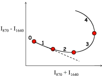
Figure 4 is a schematic plot to show the above distinct spec-tral signatures found in those three cases. This plot is drawn based on 1-D plane-parallel radiative transfer calculations. In this plot, we define 5 regimes on the DIF vs. SUM plane. These regimes are:
Fig. 4. The modeled track of the sum and difference of intensi-ties (I870andI1640)as the cloud optical depth is varied from zero (point labeled 0) to 15. Model used is DISORT (one-dimensional plane-parallel radiative transfer). Red dots, corresponding to dif-ferent cloud optical depths, separate the regimes discussed in the text. Regime 0 (a single point) represents a cloud-free condition. Regime 1 is the transition between clear and cloudy (Regimes 2–4). The dashed line is drawn to emphasize the linearity in Regime 1.
– Regime 1 corresponds to transition zones in which cloud optical depthτ up to∼0.2. In this regime, SUM increases, but DIF decreases. The relationship between DIF and SUM is linear. (In cases of very large SZAs and small cloud droplets, the slope could be also posi-tive. See Sect. 4.2.)
– Regime 2 corresponds to areas with very thin clouds (τ up to∼1). This regime is same as Regime 1, but the relationship between SUM and DIF is no longer linear. – Regime 3 corresponds to areas with thin clouds (τ up to
∼5). In this regime, both SUM and DIF increase, and the relationship between two is nonlinear.
– Regime 4 corresponds to areas with thicker clouds (τ >5). In this regime, SUM decreases while DIF increases and the relationship between two is strongly nonlinear.
Physical interpretations of these radiative signature regimes are discussed next.
4 Physics of radiative transfer behind the spectral sig-natures
For plane-parallel clouds over a Lambertian surface, any ground-based measurement of radianceI can be expressed as the sum of the downward radiation calculated over a non-reflecting (black) surface and the radiation introduced by in-teractions between clouds and the underlying surface (Box
et al., 1988). The downward radiance over a black sur-face is determined by scattering from atmospheric molecules, aerosols, and clouds. The cloud-surface interactions are de-termined by surface albedo and cloud reflective and trans-missive properties. In short, the spectral signatures in zenith radiance are primarily determined by four factors:
1. molecular (Rayleigh) and aerosol scattering, 2. in-cloud single scattering,
3. in-cloud multiple scattering, and 4. cloud-surface interactions. 4.1 Regime 0
Rayleigh and aerosol scattering dominate Regime 0. Due to stronger Rayleigh and aerosol scattering at 870 than those at 1640 nm,I870 is larger thanI1640, and thusI870−I1640is positive.
This regime strongly depends on aerosol loading and aerosol particle size. We used three different aerosol loadings: no aerosols, low aerosol optical depth (AOD, τ870a =0.05,τ1640a =0.02, ˚Angstr¨om exponent≈2/3), and high AOD (τ870a =0.15,τ1640a =0.08, ˚Angstr¨om exponent≈1). With increasing aerosol loading (Fig. 5a), Regime 0 moves to-ward the upper-right direction, i.e., bothI870+I1640(SUM) andI870−I1640(DIF) increase. The SUM increases because aerosol scattering increases at both wavelengths. The DIF in-creases because the change in AOD is larger at 870 nm than at 1640 nm.
Regime 0 also strongly depends on aerosol phase function. We show an example here by increasing aerosol particle size from effective radius of 0.25µm to 4µm for a given SZA of 45◦ (Fig. 5b). From aerosol phase functions (Fig. 6), a
larger aerosol particle size results in stronger forward scat-tering and weaker scatscat-tering at scatscat-tering angles greater than 20◦. It leads to decreases in both I870 and I1640 at larger scattering angles. However, the rate of decreases inI870is different from that inI1640. In the scattering angle range be-tween 20◦and∼50◦, the rate of decrease inI870is faster than that inI1640, and vice versa for scattering angles greater than 50◦. Therefore, at a given SZA of 45◦(i.e., scattering an-gle of 45◦), bothI
870andI1640decrease, andI870decreases faster thanI1640with increasing aerosol particle size. As a result, Regime 0 moves toward the lower-left direction with increasing aerosol particle size.
Figure 5 also shows that the locations of Regime 1 are sen-sitive to changes in aerosol properties, but the slope of the linear relationship is only weekly sensitive to those changes. We use radiative transfer calculations to understand this be-havior in next section.
4.2 Regime 1
Fig. 5.Modeled difference vs. sum of intensities, as in previous fig-ures, for clouds with various aerosol situations below the clouds.
(a)Cloud-free Regime 0 (indicated by diamonds) is affected by three assumed aerosol loadings: no aerosols, low aerosol optical depth (τ870a =0.05,τ1640a =0.02, ˚Angstr¨om exponent≈2/3), and high aerosol optical depth (τ870a =0.15,τ1640a =0.08, ˚Angstr¨om exponent ≈1). Assumed aerosol effective radius is 0.25µm. Aerosol single scattering albedo values at 870 (̟870a ) and 1640 nm (̟1640a ) are 0.97 and 0.93, respectively. Data points correspond to cloud optical depth from 0 to 0.5 in steps of 0.1, one set for each cloud drop effec-tive radius (4µm and 8µm). (b)Repeats the high aerosol loading case in (a), then adds a second case with a 16 times larger aerosol particle size (4µm) leading to the lower two curves. For the larger aerosol particle,̟870a is 0.83, and̟1640a is 0.9. Plots are based on 1D plane-parallel simulations at a SZA of 45◦.
aerosols, but also by cloud droplets. Therefore, approaching clouds leads to an increase inI870andI1640. However, the behavior of DIF vs. SUM is complex because it depends on a number of variables: the cosine of SZAµ0, the single scat-tering albedo, phase function and optical depth of aerosols and clouds. We denote them as̟λa,Pλa, andτλa, respectively for aerosols, and̟λc, Pλc, τc for clouds. The subscriptλ shows the wavelength dependency of̟ andP. Note that aerosol optical depth (AOD) is wavelength dependent, but cloud optical depth (COD) is wavelength independent at the wavelengths we used.
Ignoring molecular (Rayleigh) scattering, the total optical depth is given as:
τλ=τλa+τ c.
(3) Using the single-scattering approximation and assuming a unit incident flux at the top of the atmosphere, the downward zenith radiance is derived as (Thomas and Stamnes, 2002, p. 219):
Iλ∝̟λ·Pλ· µ0 1−µ0
[exp(−τλ)−exp(−τλ/µ0)], (4a) where̟λ andPλ are the total single scattering albedo and phase function. For a very small optical depth, Eq. (4a) can be simplified as
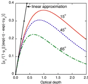
Iλ∝̟λ·Pλ·τλ. (4b) Figure 7 illustrates the right side of Eqs. (4a) and (4b) with ̟λ=1 andPλ=1 for three SZAs: 15◦, 45◦and 60◦. Compar-ing curves of Eq. (4a) with the straight line of Eq. (4b), we
Fig. 6. Aerosol scattering phase functions at wavelengths of 870 and 1640 nm for two effective particle sizes (0.25 or 4µm). The dash-dot line corresponds to a 45◦scattering angle.
Fig. 7. The right-hand side of Eqs. (4a) and (4b) with̟λ=1 and Pλ=1 vs. cloud optical depth in the single scattering approximation at solar zenith angles of 15◦, 45◦and 65◦. The straight line is the linear approximation.
see that the linear approximation is good for small optical depths up to∼0.1–0.2, depending onµ0.
Let us first assume that cloud droplets are the only scatter-ers in Regime 1. Then, because̟870c =1, Eq. (4b) determines the ratio of DIF to SUM as:
I870−I1640
I870+I1640
=P c 870−̟
c 1640P
c 1640 P870c +̟1640c P1640c =
1−̟1640c ·χ 1+̟1640c ·χ, (5) whereχis the ratio betweenP1640c andP870c , i.e.,
χ=χ µ0;rc,eff= P1640c
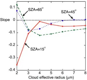
Fig. 8. Model calculations of the slope of the I870−I1640 vs. I870+I1640relationship as a function of cloud drop effective radius.
whererc,effis the cloud droplet effective radius. Equation (5) shows that the ratio is independent of cloud optical depth. It follows from here that at a givenµ0the slope of the DIF vs. SUM relationship plane is fully determined by cloud drop size in the case of τλa=0. Figure 8 shows the dependence of the slope on cloud droplet effective radius for threeµ0 values. We see that for small droplets less than 4µm, the slope derived from Eq. (5) is very sensitive to droplet size while it asymptotes for larger droplets. We also notice that at smallerµ0, the slope can be positive when cloud effective radius is very small (<2.5µm).
Now we assume a more general case ofτλa>0. Then in the frame of linear approximation Eq. (4b), Eq. (5) can be rewritten as
I870−I1640 I870+I1640 =
a−+(P870c −̟1640c P1640c )·τc
a++(P870c +̟1640c P1640c )·τc
, (7) where
a±=̟870a P870a τ870a ±̟1640a P1640a τ1640a . (8)
From Eq. (7), we see that DIF vs. SUM is a linear function. In addition, as shown in Appendix A, the slope of the linear function is:
Slope=P c
870−̟1640c P1640c P870c +̟1640c P1640c =
1−̟1640c ·χ
1+̟1640c ·χ (9)
whereχ is defined in Eq. (6). This slope is the same as that in the special case ofτλa=0 (Eq. 5). It shows that the slope is determined by cloud drop size only and independent of aerosol properties, which has been observed in Fig. 5.
Thus, assuming constant aerosol optical depth and con-stant effective sizes of cloud droplets and aerosol particles, Regime 1 shows a linear relationship between DIF and SUM as:
DIF =a+b·SUM, (10)
where as a first approximation, interceptais determined pri-marily by aerosol properties, and slopebby cloud properties, defined in Eq. (9). It shows that the linear relationship nicely separates aerosol and cloud effects intoaandb, respectively. However, aerosol properties are not the sole factor that would affect the intercepta. For the same aerosol properties, the Sun’s relative location with respective to clouds could change the interceptathrough 3-D radiative effects. Case 1 (Fig. 1) is the perfect example, showing that the Sun’s location in-troduces a difference in the intercept for the two transition periods.
Note that this linear relationship becomes less pronounced with increasing cloud optical depth, in which first the linear approximation (Eq. 4b) and then the single scattering approx-imation (Eq. 4a) is no longer held. Generally, the relationship remains linear at COD smaller than∼0.2 depending onµ0. 4.3 Regime 2–4
Because our main purpose here is to study the transition zone, the detailed description and simulations of Regime 2–4 are beyond the scope of the paper. Hence we briefly highlight main features for each regime. For the difference and the sum between 670 nm and 870 nm we can reference to Marshak et al. (2004) and Chiu et al. (2006).
Regime 2 is a continuation of Regime 1 in which in-cloud single scattering dominates. However, unlike Regime 1, the linear approximation Eq. (4b) is no longer valid in Regime 2 and radiances show a non-linear relationship with increasing optical depth (as shown in Fig. 7).
In-cloud multiple scattering and cloud-surface interactions dominate Regime 3 and 4. Equations (4a) and (4b) are no longer valid in these two regimes. In Regime 3, cloud optical depths are typically less than 4–5. This regime is in a sit-uation in which in-cloud multiple scattering dominates and surface-cloud interaction starts playing an important role. Recall that the surface-cloud interactions increase zenith ra-diance. Because the surface is brighter at 870 nm than at 1640 nm, I870 increases faster thanI1640, and thus the DIF increases with increasing COD.
Finally, Regime 4 associates with larger cloud optical depths (>5). Because less transmission gets through thicker clouds, zenith radiances at 870 and 1640 nm decrease. Simi-lar to Regime 3,I870increases faster thanI1640due to cloud-surface interactions. As a result, SUM gradually decreases while DIF increases.
5 Discussion
further discuss whether these assumptions are realistic, we review cloud microphysical measurements and some theo-retical studies in more details.
A number of studies showed that liquid water content in-creased when approaching clouds (Paluch and Baumgardner, 1989; Stith, 1992; Blyth et al., 2005). The increase of liquid water content is the result of either/both increase in droplet number concentration or/and effective radius. Which pro-cess dominates? Recall that in all cases we observed, zenith radiances sharply increased from cloud-free to cloudy ar-eas (Figs. 1c, 2c, 3c). An incrar-ease of number concentration with constant effective radius leads directly to the increase of cloud optical depth and thus of zenith radiance. The assump-tion of a constant effective radius is also consistent with the theory of inhomogeneous mixing that results in fast evap-oration of droplets of all sizes leaving effective radius un-changed (e.g., Baker et al., 1980; Freud et al., 2008). There-fore, as a very first approximation, our assumption of con-stant effective radius seems realistic.
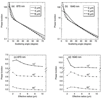
Let us now assume that effective radius increases when clouds approach. According to Eq. (4b) zenith radiance is proportional to a product of cloud optical depth and cloud scattering phase function. Cloud optical depth is propor-tional to the droplet concentration and the square of droplet size. The phase function, in general, has a non-monotonic dependency on effective radius (Fig. 9). Because it is more likely that droplets are small in the transition zone, we fo-cus on drop size from 2 to 4µm. For these droplet sizes, at SZA of 15◦, the scattering phase function changes slightly at
870 nm (Fig. 9c), but decreases sharply at 1640 nm (Fig. 9d). Therefore, no matter whether the number of droplet number concentration increases or remains unchanged, the decrease in phase function at 1640 nm leads to a slower increase in zenith radiance at 1640 nm than that at 870 nm. This contra-dicts SWS observations of Case 2.
We have assumed that aerosol particle size and optical depth remain unchanged in our theoretical derivations. How-ever, depending on aerosol compositions, aerosol extinction coefficients and sizes could increase dramatically around cloud edges because of increasing uptake of water vapor (Kotchenruther et al., 1999; Clarke et al., 2002; Loeb and Manalo-Smith, 2005; Zhang et al., 2005). Recent obser-vations from an airborne HSRL (High Spectral Resolution Lidar) have demonstrated that when approaching clouds, aerosol optical depth and extinctions could increase by 10% and 20%, respectively (Su et al., 2008). More detailed model simulations are required to understand how these changes in aerosol optical properties modulate spectral signatures of SWS in the transition zone.
Radiative signatures in the transition zone are character-ized not only by changes in aerosol and cloud properties, but also by the 3-D cloud effects (e.g., Wen et al., 2007). As shown in our cases, these effects could enhance zenith radi-ance, depending on sun-cloud-radiometer locations. In ad-dition, the field of view (FOV) of the SWS is 1.4◦. When
Fig. 9.Cloud phase functions for wavelength 870 nm (left column) and 1640 nm (right column). Top row shows phase functions versus scattering angle for effective cloud drop radii 2, 4, 8µm. Bottom row shows phase functions at specific angles versus effective drop radius; the angles chosen are the same as the solar zenith angles in Cases 1–3 for the purpose of understanding single-scattering behav-ior.
the FOV is not fully covered by clouds or by clear-sky, ra-diative signatures could be affected as well. For more details see Chiu et al. (2006).
6 Summary
To the naked eye, clouds appear to have sharp boundaries. But this is merely an illusion. Cloud boundaries are actu-ally somewhat fuzzy, with the transition from cloud to clear stretching over as little as 50 m to as much as several hun-dred meters. Within this transition zone, strong but poorly understood aerosol-cloud interactions are taking place. Re-mote sensing instruments can probe this transition zone, but the picture they paint depends on their sensitivity, their tem-poral and spatial resolution, and the thresholds chosen to dis-tinguish clear from cloudy areas. Fuzzy cloud boundaries create major headaches for studies of aerosol indirect ef-fect and aerosol radiative forcing – especially when, as with most satellite instruments, spatial resolution is too poor to re-solve the transition zone. That argues strongly for the use of ground-based instruments with spatial resolution on the order of meters, and temporal resolution better than a few seconds, to study the transition zone.
with 1-s time resolution. We have used two wavelengths, 870 and 1640 nm, from the SWS spectra to study the tran-sition zone on the sides of clouds. These two wavelengths provide information about optical depth and particle size and are nearly free of the confounding effect of Rayleigh scatter-ing.
We find, when we plot the difference (DIF) of the radi-ances at these two wavelengths versus their sum (SUM), that the trajectory followed during the cloud-free to cloud transi-tion has universal characteristics. In particular, this trajectory segments naturally into five regimes, which we number 0 to 4. In this paper we focus on Regime 0, the cloud-free area, and Regime 1, the transition zone which we define by a linear relationship between SUM and DIF.
Regime 0, the starting point of the trajectory, is deter-mined mainly by aerosol scattering and to a lesser extent by Rayleigh scattering. We find that Regime 1 has a width of 50 to 150 m. Other investigators, whose work was summarized in the Introduction, find larger values for this width, rang-ing up to several km, due to entirely different definitions of “transition zone”. In Regime 1, the trajectory is mainly deter-mined by single scattering from aerosol particles and cloud droplets. In this limiting case of single scattering, which holds only for optical depths below 0.2 or so, we proved from radiative transfer theory that there should be a linear rela-tionship between the sum and difference of zenith radiances at wavelengths of 870 and 1640 nm. We in fact observed this linear behavior in all the SWS observations meeting the small optical depth criterion. The linear behavior allows us to neatly separate effects of aerosols and clouds; the intercept of the line is mostly determined by aerosol optical depth and size while the slope of the line is mostly determined by cloud droplet size.
When we tried to quantitatively interpret the slope of the linear relationship observed in Regime 1, we found that the assumption of decreasing droplet sizes away from cloud boundaries was inconsistent with the SWS data. The data was much more consistent with constant droplet sizes across the transition zone. This suggests that the hypothesis of in-homogeneous mixing holds across the transition zone.
Appendix A
The slope of the linear relationship between SUM and DIF for a general case of τλa>0 is derived as follows. From Eqs. (4b) and (7), we get
I870+I1640= a++c+τc
·k;
I870−I1640= a−+c−τc·k, (A1)
wherekis a proportionality constant, a±=̟870a P870a τ870a ±̟1640a P1640a τ1640a ;
c±=P870c ±̟1640c P1640c . (A2)
Let us denote
x=I870+I1640, y= I870−I1640,andt=τc. (A3) Then, fort1=t+1t, we have
x1=
a++c+(t+1t )·k=x+1x;
y1=a−+c−(t+1t )·k=y+1y, (A4)
where1x=c+1t·k and1y=c−1t·k. It follows from here
that Slope=1y
1x= c−
c+
=P c
870−̟1640c P1640c
P870c +̟1640c P1640c . (A5) Acknowledgements. This research was supported by the Office of Science (BER, US Department of Energy, Interagency Agreement No. DE-AI02-08ER64562, DE-AI02-95ER61961, and DE-FG02-08ER54564) as part of the ARM program.
Edited by: T. Garrett
References
Ackerman, S. A., Strabala, K. I., Menzel, W. P., Frey, R. A., Moeller, C. C., and Gumley, L. E.: Discriminating clear sky from clouds with MODIS, J. Geophys., Res., 103, 32141—32158, 1998.
Allan, J. D., Baumgardner, D., Raga, G. B., Mayol-Bracero, O. L., Morales-Garc´ıa, F., Garc´ıa-Garc´ıa, F., Montero-Mart´ınez, G., Borrmann, S., Schneider, J., Mertes, S., Walter, S., Gysel, M., Dusek, U., Frank, G. P., and Kramer, M.: Clouds and aerosols in Puerto Rico – a new evaluation, Atmos. Chem. Phys., 8, 1293– 1309, 2008,
http://www.atmos-chem-phys.net/8/1293/2008/.
Baker, M. B., Corbin, R. G., and Latham, J.: The influence of en-trainment on the evolution of cloud droplet spectra: I. A model of inhomogeneous mixing, Q. J. R. Meteorol. Soc., 106, 581–598, 1980.
Berendes, T. A., Berendes, D. A., Welch, R. M., Dutton, E. G., Uttal, T., and Clothiaux, E. E.: Cloud cover comparisons of the MODIS daytime cloud mask with surface instruments at the North Slope of Alaska ARM site, IEEE. Trans. Geosci. Remote Sens., 42, 2584–2593, 2004.
Blyth, A. M., Lasher-Trapp, S. G., and Cooper, W. A.: A study of thermals in cumulus clouds, Q. J. Roy. Meteor. Soc., 131, 1171– 1190, 2005.
Box, M. A., Gerstl, S. A. W., and Simmer, C.: Application of the adjoint formulation to the calculation of atmospheric radiative effects, Beitr. Phys. Atmos., 61, 303–311, 1988.
Brenguier, J.-L., Bourrianne, T., Coelho, A. D., Isbert, J., Peytavi, R., Trevarin, D., and Weschler, P.: Improvements of droplet size distribution measurements with the Fast-FSSP (Forward Scatter-ing Spectrometer Probe), J. Atmos. Oceanic Techno., 15, 1077– 1090, 1998.
Charlson, R. J., Ackerman, A. S., Bender, F. A.-M., Anderson, T. L., and Liu, Z.: On the climate forcing consequences of the albedo continuum between cloudy and clear air, Tellus B, 59, 715–727, doi:10.1111/j.1600-0889.2007.00297.x, 2007.
Chiu, J. C., Marshak, A., Knyazikhin, Y., Wiscombe, W. J., Barker, H. W., Barnard, J. C., and Luo, Y.: Remote sensing of cloud properties using ground-based measurements of zenith radiance, J. Geophys. Res., 111, D16201, doi:10.1029/2005JD006843, 2006.
Clarke, A. D., Howell, S., Quinn, P. K., Bates, T. S., Ogren, J. A., Andrews, E., Jefferson, A., Massling, A., Mayol-Bracero, O., Maring, H., Savoie, D., and Cass, G.: INDOEX aerosol: A comparison and summary of chemical, microphysical, and opti-cal properties observed from land, ship, and aircraft, J. Geophys., Res., 107(D19), 8033, doi:10.1029/2001JD00572, 2002. Clothiaux, E. E., Ackerman, T. P., Mace, G. G., Moran, K. P.,
Marc-hand, R. T., Miller, M. A., and Martner, B. E.: Ojbective deter-mination of cloud heights and radar reflectivities using a combi-nation of active remote sensors at the ARM CART sites, J. Appl. Meteorol., 39, 645–665, 2000.
Coakley, J. A., Friedman, M. A., and Tahnk, W. R.: Retrieval of cloud properties for partly cloudy imager pixels, J. Atmos. Oceanic Techno., 22, 3–17, 2005.
Davis, A., Marshak, A., Gerber, H., and Wiscombe, W. J.: Horizon-tal structure of marine boundary layer clouds from centimeter to kilometer scales, J. Geophys. Res., 104, 6123–6144, 1999. Diner, D. J., Ackerman, T. P., Anderson, T. L., Bosenberg, J.,
Braverman, A. J., Charlson, R. J., Collins, W. D., Davies, R., Holben, B. N., Hostetler, C. A., Kahn, R. A., Mar tonchik, J. V., Menzies, R. T., Miller, M. A., Ogren, J. A., Penner, J. E., Rasch, P. J., Schwar tz, S. E., Seinfeld, J. H., Stephens, G. L., Torres, O., Travis, L. D., Wielicki, B. A., and Yu, B.: PARAGON – an in-tegrated approach for characterizing aerosol climate impacts and environmental interactions, B. Am. Meteorol. Soc., 85, 1491– 1501, 2004.
Freud, E., Rosenfeld, D., Andreae, M. O., Costa, A. A., and Artaxo, P.: Robust relations between CCN and the vertical evolution of cloud drop size distribution in deep convective clouds, Atmos. Chem. Phys., 8, 1661–1675, 2008,
http://www.atmos-chem-phys.net/8/1661/2008/.
Gomez-Chova, L., Camps-Valls, G., Calpe-Maravilla, J., Guan-ter, L., and Moreno, J.: Cloud-screening algorithm for EN-VISAT/MERIS multispectral images, IEEE. Trans. Geosci. Re-mote Sens., 45, 4105–4118, 2007.
Holben, B. N., Eck, T. F., Slutsker, I., Tanre, D., Buis, J. P., Set-zer, A., Vermote, E., Reagan, J. A., Kaufman, Y. J., Nakajima, T., Lavenu, F., Jankowiak, I., and Smirnov, A.: AERONET – A federated instrument network and data archive for aerosol char-acterization, Remote Sens. Environ. 66, 1–16, 1998.
Joseph, J. H. and Cahalan, R. F.: Nearest neighbor spacing of fair weather cumulus, J. Appl. Meteor., 29, 793–805, 1990. Knyazikhin, Y., Miessen, G., Panfyorov, O., and Gravenhorst, G.:
Small-scale study of three-dimensional distribution of photosyn-thetically active radiation in a forest, Agric. For. Meteorol., 88, 215–239, 1997.
Koren, I., Oreopoulos, L., Feingold, G., Remer, L. A., and Altaratz, O.: How small is a small cloud?, Atmos. Chem. Phys., 8, 3855– 3864, 2008,
http://www.atmos-chem-phys.net/8/3855/2008/.
Koren, I., Remer, L. A., Kaufman, Y. J., Rudich, Y., and Martins, J. V.: On the twilight zone between clouds and aerosols, Geophys. Res. Lett., 34, L08805, doi:10.1029/2007GL029253, 2007. Kotchenruther, R. A., Hobbs, P. V., and Hegg, D. A.:
Humidifica-tion factors for atmospheric aerosols off the mid-Atlantic coast of the United States, J. Geophys. Res., 104(D2), 2239–2251, 1999. Lane, D. E., Goris, K., and Somerville, R. C. J.: Radiative trans-fer through broken clouds: observations and model validation, J. Climate, 15, 2921–2933, 2002.
Loeb, N. G. and Manalo-Smith, N.: Top-of-atmosphere direct radia-tive effect of aerosols over global oceans from merged CERES and MODIS observations, J. Climate, 18, 3506–3526, 2005. Long, C. N. and Ackerman, T. P.: Identification of clear skies
from broadband pyranometer measurements and calculation of downwelling shortwave cloud effects, J. Geophys. Res., 105D12, 15609–15626, 2000.
Long, C. N., Slater, D. W., and Tooman, T.: Total Sky Imager Model 880 status and testing results, ARM Technical Report ARM TR-006, US Department of Energy, Washington, D.C., 2001. Long, C. N., Ackerman, T. P., Gaustad, K. L., and Cole, J. N.
S.: Estimation of fractional sky cover from broadband short-wave radiometer measurements, J. Geophys. Res., 111, D11204, doi:10.1029/2005JD006475, 2006a.
Long, C. N., Sabburg, J. M., Calbo, J., and Pages, D.: Retriev-ing cloud characteristics from ground-based daytime color all-sky images, J. Atmos. Oceanic Technol., 23, 633-652, 2006b. Lu, M.-L., Wang, J., Freedman, A., Jonsson, H. H., Flagan, R. C.,
McClatchey, R. A., and Seinfeld, J. H.: Analysis of humidity ha-los around trade wind cumulus clouds, J. Atmos. Sci., 60, 1041– 1059, 2003.
Marshak, A., Knyazikhin, Y., Evans, K. D., and Wiscombe, W. J.: The “RED versus NIR” plane to retrieve broken-cloud op-tical depth from ground-based measurements, J. Atmos. Sci., 61, 1911–1925, 2004.
Marshak, A., Wen, G., Coakley, J., Remer, L., Loeb, N. G., and Cahalan, R. F.: A simple model for the cloud adjacency effect and the apparent bluing of aerosols near clouds, J. Geophys. Res., 113, D14S17, doi:10.1029/2007JD009196, 2008.
Martins, J. V., Tanr´e, D., Remer, L. A., Kaufman, Y. J., Mattoo, S., and Levy, R.: MODIS cloud screening for remote sensing of aerosol over oceans using spatial variability, Geophys. Res. Lett., 29(12), 8009, doi:10.1029/2001GL013252, 2002.
Miller, M. A., Johnson, K. L., Troyan, D. T., Clothiaux, E. E., Mlawer, E. J., and Mace, G. G.: ARM value-added cloud prod-ucts: description and status, Proceedings of the 13th ARM Science Team Meeting, 31 March to 4 April 2003, Broom-field, Colorado, available at: http://www.arm.gov/publications/ proceedings/conf13/extended abs/miller-ma.pdf, 2003. Paluch, I. R. and Baumgardner, D. G.: Entrainment and fine-scale
mixing in a continental convective cloud, J. Atmos. Sci., 46, 261– 278, 1989.
Perry, K. D. and Hobbs , P. V.: Influences of isolated cumulus clouds on the humidity of their surroundings, J. Atmos. Sci., 53, 159– 174, 1996.
Platt, C. M. R. and Gambling, D. J.: Laser radar reflexions and downward infrared flux enhancement near small cumulus clouds, Nature, 232, 182–185, 1971.
Schaaf, C. B., Gao, F., Strahler, A. H., Lucht, W., Li, X .W., Tsang, T., Strugnell, N, C., Zhang, X. Y., Jin, Y. F., Muller, J. P., Lewis, P., Barnsley, M., Hobson, P., Disney, M., Rober ts, G., Dun-derdale, M., Doll, C., d’Entremont, R. P., Hu, B. X., Liang, S. L., Privette, J. L., and Roy, D.: First operational BRDF, albedo nadir reflectance products from MODIS, Remote Sens. Environ., 83, 135–148, 2002.
Stephens, G. L., Vane, D. G., Boain, R. J., Mace, G. G., Sassen, K., Wang, Z. E., Illingworth, A. J., O’Connor, E. J., Rossow, W. B., Durden, S. L., Miller, S. D., Austin, R. T., Benedetti, A., and Mitrescu, C.: The CloudSat Mission and the A-Train – A new dimension of space-based observations of clouds and precipitation, B. Am. Meteorol. Soc., 83, 1771–1790, 2002. Stith, J. L.: Observations of cloud-top entrainment in cumuli, J.
Atmos. Sci., 49, 1334–1347, 1992.
Su, W., Schuster, G. L., Loeb, N. G., Rogers, R. R., Fer-rare, R. A., Hostetler, C. A., Hair, J. W., and Obland , M. D.: Aerosol and cloud interaction observed from high spec-tral resolution lidar data, J. Geophys. Res., 113, D24202, doi:10.1029/2008JD010588, 2008.
Taylor, T. E., L’Ecuyer, T. S., Slusser, J. R., Stephens, G. L., and Goering, C. D.: An operational retrieval algorithm for determin-ing aerosol optical properties in the ultraviolet, J. Geophys. Res., 113, D03201, doi:10.1029/2007JD008661, 2008.
Thomas, G. E. and Stamnes, K.: Radiative transfer in the atmo-sphere and ocean, Cambridge University Press, 517 pp., 2002. Turner, D. D., Clough, S. A., Lijegren, J. C., Clothiaux, E. E.,
Cady-Pereira, K. E., and Gaustad, K. L.: Retrieving liquid water path and precipitable water vapor from the atmospheric radiation mea-surement (ARM) microwave radiometers, IEEE. Trans. Geosci. Remote Sens., 45, 3680–3690, 2007.
Walte-Shea, E. A. and Norman, J. M.: Leaf optical properties, in: Photon-Vegetation Interactions: Applications in Plant Physiol-ogy and Optical Remote Sensing, edited by: Myneni, R. B. and Ross, J., Springer-Verlag, 229–251, 1991.