www.clim-past.net/10/1817/2014/ doi:10.5194/cp-10-1817-2014
© Author(s) 2014. CC Attribution 3.0 License.
Coupled ice sheet–climate modeling under glacial and pre-industrial
boundary conditions
F. A. Ziemen1,2,*, C. B. Rodehacke1,**, and U. Mikolajewicz1
1Max Planck Institute for Meteorology, Bundesstr. 53, 20146 Hamburg, Germany
2International Max Planck Research School on Earth System Modelling (IMPRS), Bundesstr. 53, 20146 Hamburg, Germany *now at: Geophysical Institute, University of Alaska, Fairbanks, USA
**now at: Danish Meteorological Institute, Copenhagen, Denmark
Correspondence to: F. A. Ziemen ([email protected])
Received: 8 January 2014 – Published in Clim. Past Discuss.: 11 February 2014 Revised: 28 August 2014 – Accepted: 29 August 2014 – Published: 7 October 2014
Abstract. In the standard Paleoclimate Modelling Inter-comparison Project (PMIP) experiments, the Last Glacial Maximum (LGM) is modeled in quasi-equilibrium with atmosphere–ocean–vegetation general circulation models (AOVGCMs) with prescribed ice sheets. This can lead to in-consistencies between the modeled climate and ice sheets. One way to avoid this problem would be to model the ice sheets explicitly. Here, we present the first results from coupled ice sheet–climate simulations for the pre-industrial times and the LGM.
Our setup consists of the AOVGCM
ECHAM5/MPIOM/LPJ bidirectionally coupled with the Parallel Ice Sheet Model (PISM) covering the Northern Hemisphere. The results of the pre-industrial and LGM simulations agree reasonably well with reconstructions and observations. This shows that the model system adequately represents large, non-linear climate perturbations.
A large part of the drainage of the ice sheets occurs in ice streams. Most modeled ice stream systems show recur-ring surges as internal oscillations. The Hudson Strait Ice Stream surges with an ice volume equivalent to about 5 m sea level and a recurrence interval of about 7000 yr. This is in agreement with basic expectations for Heinrich events. Un-der LGM boundary conditions, different ice sheet configura-tions imply different locaconfigura-tions of deep water formation.
1 Introduction
The understanding of past climates is a major challenge. Well-documented, non-linear climate changes can be stud-ied by modeling past climates that differ greatly from the present-day climate. This improves the understanding of the climate system (e.g., Valdes, 2011; Braconnot et al., 2012).
The last glacial climate differed greatly from the present-day climate, although the last glacial is very recent from a geological perspective. Therefore, the proxy coverage and dating accuracy are comparatively good. The climate differ-ences between the last glacial and the present mainly stem from the reduced greenhouse gas content of the atmosphere and from the massive ice sheets covering the continents of the Northern Hemisphere (Rind, 1987; Kim, 2004; Abe-Ouchi et al., 2007; Pausata et al., 2011). The ice sheets were at their maximum volume about 21 000 yr ago, during the so-called Last Glacial Maximum (LGM) (e.g., Clark et al., 2009). In atmosphere–ocean general circulation models (AOGCMs), the LGM climate is commonly modeled in steady-state ex-periments (e.g., in the Paleoclimate Modelling Intercompar-ison Project, PMIP).
other. To obtain ice sheets that are consistent with the mod-eled climate, it is essential to overcome this method and to model the ice sheets interactively. We took exactly this step. We extended the PMIP-2 setup by an interactively coupled ice sheet model (ISM), and studied the climate as well as the ice sheets in this self-consistent system with its increased complexity. By comparing the modeled ice sheets with re-constructions, we can critically assess our model system.
An interactively coupled ice sheet–climate model opens the possibility of studying the interactions between ice sheets and the climate system. In the light of the recently observed changes in the ice sheets and their potential impact on fu-ture sea level rise (e.g., Vaughan et al., 2013), such studies become increasingly relevant for predicting future climate change. The large ice masses and the possibility of compar-ing the model results to proxy data make the LGM an ideally suited time period for studying ice–climate interactions.
The long intrinsic timescales of ice sheets make the as-sumption of the ice sheets being in equilibrium with the cli-mate problematic. These timescales also require long simu-lations that are challenging to perform with AOGCMs. Com-plicating the modeling further, most of the snowfall and melt occurs in a narrow band along the ice sheet margin. In prin-ciple, the margin zone calls for high-resolution modeling, while the long timescales prohibit this. The discrepancy be-tween the need for high-resolution modeling and long time spans leads to a variety of strategies (see the reviews by Pol-lard, 2010, and Vizcaíno, 2014).
At the fast and simple end of the model spectrum, fixed climate maps or analytical expressions are scaled by the use of a time series, either from an energy balance model or from ice core data. In earlier times, these models were used to study one glacial cycle (e.g., Pollard, 1982; Greve, 1997; Tarasov and Peltier, 1997). Advances in computing power now make it possible to model the evolution of the ice sheets over millions of years with such models (Pollard and DeConto, 2009). Tarasov et al. (2012) performed mul-tiple experiments covering the last glacial. They chose the experiments that agreed best with the proxy data and created a deglacial ice sheet chronology that is consistent with proxy data as well as with ice physics.
Zweck and Huybrechts (2003) forced an ISM by interpo-lating between modeled climate states for LGM and mod-ern boundary conditions using Greenland ice core data as weighting coefficients. Charbit et al. (2007) compared the effect of different AGCMs on the same ISM using a simi-lar approach. They found the Eurasian ice sheets to be more sensitive to the choice of the climate model than the Lau-rentide. Abe-Ouchi et al. (2007, 2013) used multiple experi-ments performed with the same climate model to create a sta-tistical model that accounts for changes in greenhouse gases, orbital parameters, and ice sheets separately. They coupled this model to an ISM and performed simulations of the last glacial cycle. They found the snow-albedo feedback and the temperature lapse rate to be the most important feedback
fac-tors. For the deglaciation, the delayed isostatic rebound of the lithosphere played a key role.
Another approach uses earth system models of interme-diate complexity (EMICs) and optionally downscales the fields for the ISM in an intermediate energy balance model or energy-moisture balance model. Calov et al. (2002) used such a setup, and obtained binge–purge oscillations of the Laurentide Ice Sheet resembling Heinrich events as internal oscillations of the ice sheet. Wang and Mysak (2002) and Calov et al. (2005) studied the feedbacks and bifurcations during the glacial inception, or more recently, full glacial cy-cles (Bonelli et al., 2009; Ganopolski et al., 2010; Ganopol-ski and Calov, 2011). Recently, Heinemann et al. (2014) per-formed transient simulations starting at 80 kyr BP and ob-tained a much smaller LGM Fennoscandian Ice Sheet in the transient simulation than in a steady state sensitivity study. This shows that the Fennoscandian Ice Sheet was not in an equilibrium state at the LGM.
The most expensive approaches use coupled AOGCM– ISM systems. While the EMIC or energy balance model based methods can cover long time spans with reasonable effort, they strongly simplify the atmosphere and/or ocean dynamics. In contrast, AOGCMs suffer from high computa-tional costs but provide a detailed representation of the atmo-sphere and ocean dynamics. To bridge the long time spans, most research groups couple the models asynchronously. In this method, the climate model is run for a period of one to fifty years, and then the climate is used to drive the ice sheet for a substantially longer period. The resulting ice sheet is fed back into the climate model and the cycle is started over (Pollard et al., 1990; Ridley et al., 2005; Mikolajewicz et al., 2007a; Gregory et al., 2012).
by Gregory et al. (2012) used the AOGCM FAMOUS, a fast version of HADCM3, in combination with the ISM GLIM-MER to study the last glacial inception. They found a strong dependence of the ice volume on the way the ice-albedo feed-back is treated in the coupling. None of the published studies addressed LGM conditions.
We have coupled a coarse-resolution AOVGCM (ECHAM5/MPIOM/LPJ; Mikolajewicz et al., 2007b) interactively with a state-of-the-art ISM, the modified Par-allel Ice Sheet Model (mPISM). The coupling is performed bidirectionally, and without flux corrections nor anomaly methods. Our intention is to apply the model system for transient long-term simulations of, e.g., the last termination. As a first step, we will validate here the ability of the model system to reproduce the climate of two time slices, which are sufficiently different that they allow us also to validate the model’s sensitivity to perturbations. We chose the pre-industrial and the last glacial maximum. The only factors we varied between the LGM and the pre-industrial setup were the greenhouse gas concentrations, the orbitals and the shapes of the continents. We let the models evolve freely sufficiently long to be largely independent of the initial state. We study the behavior of the climate system and compare the model results to observations and proxy data. As the model system is new, this paper also has a strong focus on the description of the model system and the coupling between the different components.
We describe the models, the necessary modifications, the coupling and the setups in Sect. 2, analyze the mean states of the experiments in Sect. 3, and summarize the main findings and draw the conclusions in Sect. 4.
2 Model description and setups
The AOVGCM has been applied before coupled to the ISM SICOPOLIS for studies of the future evolution of the Green-land and Antarctic ice sheets (Mikolajewicz et al., 2007b; Vizcaíno et al., 2010). For this study, we have switched to PISM, and changed various aspects of the coupling. The models and the coupling will be described in the following.
2.1 ECHAM5/MPIOM/LPJ
The atmospheric component of the coupled model is ECHAM5 (Roeckner et al., 2003), a spectral atmosphere general circulation model. For long-term simulations, the triangular spectral truncation at wavenumber 31 (T31, ∼3.75◦) in combination with 19 vertical hybrid-σ-levels reaching up to 10 hPa is a compromise between computa-tional demand and accuracy. This setup is therefore em-ployed in all experiments described in the following. The land hydrology scheme (HD model, Hagemann and Düme-nil, 1998; Hagemann and Gates, 2003) operates on a 0.5◦ grid. For the HD model, we use the present-day routing
direc-tions in combination with the LGM land-sea-mask. The land surface properties are modeled using the Lund-Potsdam-Jena (LPJ) vegetation model (Sitch et al., 2003). Its use in combi-nation with ECHAM is described in Schurgers et al. (2007) and Mikolajewicz et al. (2007b).
MPIOM (Marsland et al., 2003) is a primitive equation ocean model operating on a curvilinear grid with variable resolution. In the setup employed in the following, the grid has two poles, located over Greenland and Antarctica, and a nominal resolution of 3◦. This results in an increased res-olution in the deep water formation areas, and a relatively coarse resolution in the equatorial areas.
The atmosphere and ocean are coupled using the OASIS coupler (Valcke et al., 2004). The performance of a higher-resolution version of the coupled AOGCM is described in Jungclaus et al. (2006). In the framework of the PMIP-2 the AOGCM ECHAM5/MPIOM/LPJ has been applied to the LGM. Results can be found in the PMIP-2 database at http://pmip2.lsce.ipsl.fr.
2.2 mPISM
mPISM is based on PISM version 0.3 from the University of Alaska, Fairbanks (Bueler and Brown, 2009; the PISM au-thors, 2014). PISM uses the Shallow Ice Approximation (SIA) and the Shallow Shelf Approximation (SSA) to com-pute flow velocities. It uses an enthalpy method to handle polythermal ice (Aschwanden et al., 2012). Details about the model can be found in the literature given above. Several as-pects of the model needed to be changed for the coupling to the climate model and for obtaining pulsating ice streams. In the following, we describe the modifications of the PISM physics. For the technical changes see Ziemen (2013). We use the term PISM 0.3 when referring to the base version, mPISM when referring to the modified version, and PISM when referring to aspects of the base version that also ap-ply to the modified version. PISM-PIK (Winkelmann et al., 2011) is a branch of PISM that is developed at the Potsdam Institute for Climate Impact Research (PIK).
Following Calov et al. (2002), we use a linear sliding law with a friction coefficient of 1 m yr−1Pa−1that allows slid-ing if there is basal water and deformable sediment available to lubricate the ice sheet. The availability of the sediment is based on the data set from Laske and Masters (1997) with a cutoff value of 5 cm, and is marked in Fig. 1. The avail-ability of basal water is a prognostic quantity of PISM. We spread out half of a grid cell’s heat flux from basal friction on the cell’s eight neighbors. This slightly heats the grid cells adjacent to an ice stream.
Figure 1. Ice streams. Brownish/red colors mark the fraction of time
that a grid cell is sliding at more than 1 m yr−1. Blue marks areas where the ice is not permitted to slide due to the lack of sediments in the reconstruction of Laske and Masters (1997). Only the time when the grid cell is ice covered is taken into consideration; therefore, ice shelves are considered to be constantly sliding. Numbers match the ice stream numbering in Stokes and Tarasov (2010), and are as follows: (1) Mackenzie, (16) Ungava Bay, (18) Amundsen Gulf, (19) M’Clure Strait, (20) Gulf of Boothia, (21) Admirality Inlet, (22) Lancaster Sound, (23) Cumberland Sound, (24) Hudson Strait, (25) Laurentian. Letters mark present-day location names of mod-eled Greenland ice streams: (A) Northeast Greenland Ice Stream, (B) Kejser Franz Joseph Fjord, (C) Scoresby Sund, (D) Kangerd-lugssuaq, (E) Jakobshaven Isbrae, (F) Kong Oscar Glacier. Greek letters (α, β, γ) mark Barents Shelf ice streams.
For the bedrock deformation, we use a Local Lithosphere Relaxed Asthenosphere (LLRA) model (e.g., Le Meur and Huybrechts, 1996) with a rebound timescale of 3 kyr. We dy-namically compute the change in sea level that is caused by the ice sheets and use it to adjust the sea level in the ISM and in the climate model.
Our setup uses a Cartesian coordinate system that is a Po-lar Stereographic projection of the Northern Hemisphere, covers all areas north of 36.7◦N, and reaches south to 19.1◦N in the corners. This grid covers all Northern
Hemi-sphere regions where we can possibly expect to grow large-scale ice sheets under glacial conditions (including the Hi-malayas). The resolution is 20 km in both directions (625× 625 grid cells). Outside of the mPISM domain, we use the ICE-5G (Peltier, 2004) topography matching the time slice of interest, as in PMIP-2.
2.3 The coupling from the climate to the ice sheet
The coupling scheme between ECHAM5, MPIOM and mP-ISM computes the ice sheet mass balance and surface tem-perature from the ECHAM5 and MPIOM output, and trans-fers surface topography, glacier mask and mass fluxes from mPISM back to ECHAM5 and MPIOM. We will now lay out the path from the climate model to mPISM.
To compute the mass balance for the ice sheet, we have to use a high spatial resolution that resolves the tempera-ture distribution at the ice sheet margins. We use the 20 km grid of mPISM for the mass balance calculations. To save computational time, we compute monthly averages of the at-mospheric quantities and annual averages of the ocean vari-ables before regridding them to the ISM grid. These regrid-ded high-resolution fields are used in the ISM to determine the mass balance. The scheme we use to process tempera-tures and precipitation from ECHAM5 for the use in mPISM is based on the standard scheme employed in SICOPOLIS, which stems from Braithwaite and Olesen (1989).
To account for surface elevation differences between the two models, we correct the temperatures using a lapse rate of −5 K km−1as suggested by Abe-Ouchi et al. (2007). We use the height-corrected monthly mean temperatures to partition the precipitation into solid and liquid fractions using a linear transition between−10 and+7◦C as in Marsiat (1994). The solid fractionPsolidis used as accumulation, and the liquid fraction is discarded immediately as runoff. To account for the reduced precipitation at high altitudes, we apply a height desertification parametrization as in Budd and Smith (1979) at heights above 2000 m.
P =Psolidexp(−λ(max(hISM,2000 m)
−max(hGCM,2000 m))), (1) wherehISMis the surface height in mPISM,hGCMis the sur-face height in the climate model, andλ=log(2)/1000 m.
ice grid (which would be more computationally demanding) and the standard approach of prescribing a fixed standard deviation in the full model domain. The PDD scheme em-ploys the Calov–Greve integral method (Calov and Greve, 2005) to compute PDDs from monthly mean temperatures and standard deviations. Then, from these PDD, and the snow accumulation, the actual mass balance is computed using a standard PDD scheme (Reeh, 1991). We chose a snow melt rate of msnow=3.2 mm ice equivalent K−1day−1, an ice melt rate ofmice=12.9 mm ice K−1day−1and allow up to 60 % of the melt to refreeze in the snowpack. The ice melt rates are based on Greve et al. (1999), who chose 3 mm and 12 mm water equivalent per day and degree Celsius in North-ern Hemisphere simulations.
For the basal ice shelf melt (or growth), we use the three-equation scheme described in Holland and Jenkins (1999). This scheme computes the ice shelf basal mass balance and properties of a thin boundary layer from ocean salinity and temperature as well as the ice shelf basal temperature gradi-ent. We force this model with the annual mean temperature and salinity averaged over the top 12 layers(203 m)from the ocean model.
We employ a simple calving scheme that operates on a grid cell and its eight neighbors. If less than three of the nine cells have an ice thickness above 200 m, and the relaxed bedrock topography is below sea level, then the ice is calved. This allows shelves to grow and retreat dynamically, and prevents one grid cell wide ice tongues.
2.4 The coupling from the ice sheet to the climate
In the following, we describe how the output fields from the ISM are transferred into the atmosphere and ocean models. For the areas outside of the mPISM domain, the mPISM sur-face field is combined with a background map. The combined map is adjusted for sea level changes from the ice sheet. To keep the subgrid-scale orography consistent, the background map is smoothed with respect to the standard topography map used for ECHAM5, so it matches the roughness of the ice-free areas of the remapped mPISM topography. From this map, both the mean topography as well as subgrid-scale to-pographic variables like the maximum surface height in a grid box are calculated. Since this smoother surface would significantly change climate in comparison to the standard model setup, we upscale the subgrid surface slopes by a fac-tor of 2. Furthermore, we decrease the resolution-dependent threshold for activating the gravity wave drag parametriza-tion in ECHAM5 from the standard T31 value of 400 m to 300 m peak – mean elevation, so the gravity wave drag parametrization is active in about the same grid cells as in the original setup.
All ISM grid cells with an ice thickness above 10 m are treated as glaciated. We use conservative area remapping to interpolate the glacier mask to the ECHAM5 grid. ECHAM5 does not allow for fractional glaciation of a grid box, and
treats all grid cells with a fractional glacier mask value above 0.5 as fully glaciated. To generate a more gradual transi-tion between fully glaciated and non-glaciated grid cells, we modified the ECHAM5 albedo scheme. For grid cells that ECHAM5 considers as glaciated, the albedo is computed based on a fractional glacier cover with a background albedo of 0.25 for the non-glaciated parts of the grid cell. For those grid cells that have a glacier fraction below 0.5 and are thus considered as non-glaciated in ECHAM5, we reduce the for-est (tree cover) fraction by the glacier fraction to obtain an effective forest cover (foresteff) and compute a new back-ground albedoαeff that represents the effects of the albedo of the glaciated parts:
foresteff=(1−glacier)forest; (2)
αeff=(1−glacier) αlpj+glacierαglacier (3) where forest is the forest fraction computed by LPJ, glacier the glacier fraction from the remapped the mPISM output,
αlpj the background albedo calculated from the vegetation model, andαglacier a background albedo for melting glacier ice(0.5). The reduction of the forest fraction is important be-cause it reduces the snow-masking effect in the albedo cal-culation of ECHAM5.
The mass (fresh water) flux coupling preserves flux rates. We associate fluxes from iceberg calving and shelf basal melt with a negative enthalpy flux into the ocean, so that these processes lead to ocean cooling and/or increased sea ice formation. The net surface mass balance on the ice sheets is subtracted from the precipitation–evaporation field fed into the surface runoff model. Similarly, the effects of ice-ocean interactions are directly fed into the MPIOM’s surface scheme. All grid conversions are performed using conserva-tive remapping. In experiments with synchronous coupling, this yields perfect mass conservation.
We keep the ocean bathymetry and land sea mask constant. The freshwater fluxes change the surface height of the ocean. In ECHAM5 we reduce the land surface elevation when the sea level rises, and vice versa.
For the experiments presented in this publication, we use an asynchronous coupling scheme, where mPISM is run for 10 years while the climate model is run for 1 year between the coupling procedures. In this setup, our scheme conserves mass fluxes instead of total mass. This method has been suc-cessfully employed in previous simulations (Vizcaíno et al., 2008), and avoids overly strong freshwater forcings for the ocean model. Such forcings would arise from conserving mass and increasing the flux rates.
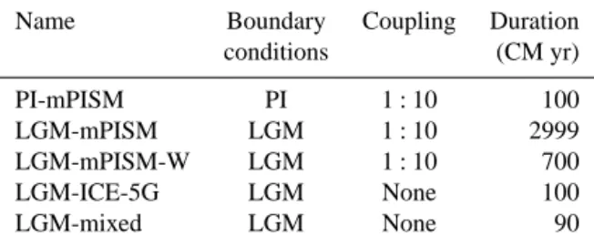
Table 1. Main experiments performed and analyzed. For the
bound-ary conditions, see Table 2. 1:10 coupling means 1 climate model (CM) year per 10 ISM years. The coupling is performed after each year of climate model integrations. For easy reference, ISM years in the coupled experiments are ten times the corresponding climate model years, thus climate model year 10 corresponds to ISM years 100 to 109.
Name Boundary Coupling Duration
conditions (CM yr)
PI-mPISM PI 1:10 100
LGM-mPISM LGM 1:10 2999
LGM-mPISM-W LGM 1:10 700
LGM-ICE-5G LGM None 100
LGM-mixed LGM None 90
new energy sources or sinks. By explicitly modeling the ice sheets, our model however is more realistic than GCM-only simulations, where the ice sheet extent is prescribed.
2.5 Setups and experiments
Our experimental strategy was to perform two coupled ex-periments, one under glacial and one under pre-industrial conditions, and to compare the results with each other and with observations and proxy data. We additionally performed three sensitivity studies under LGM conditions: LGM-ICE-5G, LGM-mPISM-W, and LGM-mixed. They are described in Sect. 3.4. We list all experiments in Table 1.
The coupling and tuning of the models required iterative improvements. To avoid costly repeated transient spinups of the LGM state, we forced the models with constant LGM conditions (Table 2). Thus, the ISM was run for more than 100 000 years under LGM conditions with increasing com-pleteness of the coupling. The climate model was started from an existing LGM state (Arpe et al., 2011) and run for 3850 years during the coupling. The last 21 500 ISM years (2150 climate model years), the models were fully cou-pled. From the resulting state, we started our main LGM ex-periment, LGM-mPISM. We integrated this experiment for 30 000 years in the ISM (3000 years in the climate model). Unless explicitly stated otherwise, we average over the full duration of this experiment in this publication.
The second main experiment is the pre-industrial control run PI-mPISM. The ISM was initialized with the present-day Greenland Ice Sheet shape using PISM’s bootstrap meth-ods. They provide an empirical guess for the temperature profile in the interior based on the surface air temperature and the geothermal heat flux at the base. The climate model was started from an existing pre-industrial state. The coupled model was spun up for 9000 years in the ISM (900 years in the climate model) and the following 1000 (100) years were analyzed.
Table 2. Boundary conditions differing between the LGM and
pre-industrial setups.
Parameter LGM Pre-industrial
Topography ICE-5G 21 ka ICE-5G 0 ka Eccentricity 0.0190 0.0167 Obliquity 22.95◦ 23.45◦ Angle of perihelion 114.4◦ 102.0◦
CO2(ppm) 185 280
N2O (ppm) 0.20 0.27
CH4(ppm) 0.35 0.67
In the coupled experiments, the coupling was performed after every year of climate model simulations (10 years of ISM simulations).
3 Results and discussion
In the following, we first discuss the pre-industrial experi-ment (PI-mPISM) and then the LGM mean state in LGM-mPISM and LGM-ICE-5G. Finally, we describe the long-term drift of the ice sheets in LGM-mPISM. The main pur-pose of PI-mPISM is to show that our setup yields reasonable results under pre-industrial boundary conditions and to pro-vide a reference state to compare the LGM climate against. We therefore limit the analysis of this experiment to key cli-mate parameters and compare those to reanalysis and obser-vational estimates. We largely draw on data for present-day conditions. These are available at high quality, and the dif-ferences to the pre-industrial climate are minor compared to the LGM effects we focus on in this study. We first discuss the state of the atmosphere, then the ocean, and finally the ice sheets.
3.1 The pre-industrial atmosphere
and 45◦N). The model shows a significant cold bias over
Siberia.
The smoothed-out T31 grid of ECHAM5 is lower than the T255 grid of ERA INTERIM in most mountain areas (the creation of the grid involves spectral smoothing and is not conservative, so the mean surface elevation is lower in a T31 grid than in reality). Differences that can directly be traced back to the lower topography in the T31 resolution of the atmosphere model are the warm biases over the Andes and the Himalayas. Over the Himalayas, typical surface altitude differences between the two model setups are about 500 to 1000 m on the T31 grid, over the Andes, they reach 2000 m, and over the southern tip of Greenland, they reach 1000 m. Assuming a lapse rate of 5 K km−1, as it is used in our cou-pling scheme, this corresponds to a 2.5–5 K temperature dif-ference over the Himalayas, 5–10 K temperature difdif-ference over the Andes, and up to 5 K temperature difference over the southern tip of Greenland.
There is a cold bias over the northern Atlantic. This is a consequence of the North Atlantic Current taking too southerly a route. Eddy-resolving modeling has been shown to improve the representation of the Gulf Stream separation and the path of the North Atlantic Current (e.g., Hurlburt and Hogan, 2000; Bryan et al., 2007), but is not yet feasible for multi-millennial simulations.
There is a strong cold bias over the Alaska Range that also occurs in stand-alone simulations (not shown) and be-comes stronger because of ice-sheet growth in the coupled setup (Fig. 3). This temperature bias, and thus the glaciation, can be reduced by increasing the climate model resolution (e.g., in the CMIP3 experiments that were performed with a technically identical climate model version), but this is not yet feasible for multi-millennial experiments.
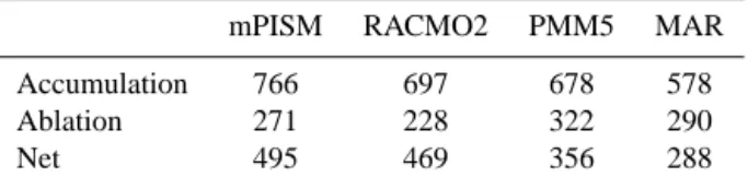
A comparison of the present-day annual mean precipita-tion data from the GPCP data set (Adler et al., 2003) with PI-mPISM (Fig. 4) shows a good agreement over Greenland. This is also reflected in the agreement of our Greenland mean surface accumulation values with those from regional mod-eling (Table 3). Over the other polar areas, the values also match closely. Most of the precipitation differences occur in the tropics and at southern mit latitudes (not shown). The differences in the tropics are standard modeling artifacts, and neither region is of special interest for this study. In the global mean, the precipitation of 1.03 m yr−1is 5 % above the GPCP estimate, while north of 45◦N, the modeled precipitation of 0.66 m yr−1is 10 % lower than the GPCP estimate.
3.2 The pre-industrial ocean
The North Atlantic Deep Water (NADW) cell of the AMOC peaks at 17.0 Sv (1 Sv=106m3s−1) at 32.5◦N and a depth of 1020 m. This agrees with the estimate of 16±2 Sv from Ganachaud (2003) and recent measurements of 18.7±2 Sv at 26.5◦N (Kanzow et al., 2010). The NADW is formed south of Greenland and in the Nordic seas (Fig. 5). The Antarctic
Table 3. Greenland surface mass balance in Gt yr−1. RACMO2, Polar MM5 (PMM5) (Box et al., 2006), and MAR (Fettweis, 2007) data are for the period 1958–2007 (RACMO2, MAR), resp. 1958– 2006 (PMM5) and are taken from Supplement S1 from Ettema et al. (2009).
mPISM RACMO2 PMM5 MAR
Accumulation 766 697 678 578
Ablation 271 228 322 290
Net 495 469 356 288
Bottom Water (AABW) cell in the Atlantic peaks at 2.9 Sv at 30◦S and a depth of 3570 m. The northward heat trans-port in the Atlantic of 0.86 PW at 23◦N is lower than the present-day estimates. Ganachaud and Wunsch (2003) ob-tain 1.27±0.15 PW at 24◦N as a result of the World Ocean Circulation Experiment (WOCE), and Johns et al. (2011) ob-tain 1.33±0.14 PW at 26◦N from the RAPID mooring array measurements. A comparison of the modeled temperatures in the Atlantic and data from WOCE (Koltermann et al., 2011) shows that, in our model, the deep water flowing southward is warmer than it is in reality. This explains why our model simulates less heat transport than the estimates derived from observations indicate, while the overturning strength is simi-lar.
The sea ice maximum and minimum extent agree very well with the long-term average of the HadISST observational data set (Rayner et al., 2003) (Fig. 3).
3.3 The pre-industrial ice sheets
Figure 3 shows the ice sheets in PI-mPISM averaged over the last 1000 yr, as well as the deviations from the reference topography. We obtain a Northern Hemisphere land ice volume of 5.9 Mio km3, corresponding to 14.9 m of sea level equivalent (SLE) (Table 4). Of this volume, 3.65 Mio km3 (9.2 m SLE) are stored in the Greenland Ice Sheet (see Fig. 6 for the mask used in the analysis). To-day’s Greenland Ice sheet has a volume of 2.9 Mio km3 (7.3 m SLE). The drift in Greenland Ice sheet volume is −14 km3yr−1. It has a two-dome structure; the main dome reaches a height of 3200 m a.s.l. (above sea level) (3300 m in reality, Bamber et al., 2001) and the southern dome reaches 2700 m a.s.l.(2900 m in reality).
Along most of the coasts of Greenland, the model grows too much ice. At the northern and northern east coast (north of 70◦N), this is largely due to practically zero ablation from
a) b) c)
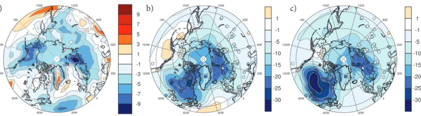
Figure 2. Annual mean SAT differences. (a) PI-mPISM – ERA INTERIM, (b) LGM-mPISM – PI-mPISM, (c) LGM-ICE-5G – PI-mPISM.
Dots show proxy data for LGM – present day from Schmittner et al. (2011) and Kim et al. (2008).
a) b)
Figure 3. Ice sheets in PI-mPISM. (a) The surface topography in
mPISM averaged over the last 1000 ice-model years of PI-mPISM. Isolines are drawn every 500 m. Ice-covered regions are colored. Over the ocean, dark gray with a red outline indicates areas with perennial ice cover (15 % level) in more than 50 % of the model years. Light gray with a dark blue-black outline indicates tempo-rary ice cover in more than 50 % of the model years. The Bering Strait appears to be ice free, because it is slightly displaced to the west in the ocean model. The orange outline marks areas that have permanent sea ice cover in more than 50 % of the years 1870 to 2010 according to the HadISST sea ice data set (Rayner et al., 2003). The light blue outline marks areas that have temporary sea ice cover in more than 50 % of these years according to HadISST. (b) The difference between the modeled pre-industrial topography and the present-day topography (ETOPO1; Amante and Eakins, 2009).
when remapping from ECHAM5 to mPISM. The mean tem-perature between a sea ice covered grid cell and a glaciated grid cell cannot allow for substantial surface melt. Therefore, the surface mass balance is positive practically all the way to the coast, while substantial ice melt would be needed to stop the glaciers before the coast. There is substantial melt near the western coast where two ECHAM5 grid cells with a glacier fraction below 0.5 remain that are considered as
Table 4. Ice sheet volumes and their changes in PI-mPISM averaged
over the last 1000 yr of the simulation. Greenland volume: Bamber et al. (2001). Glaciers outside of Greenland and Antarctica are esti-mated between 0.05 and 0.13 Mio km3in Lemke et al. (2007).
Volume (Mio km3) Drift (km3yr−1) Ice sheet Present day mPISM mPISM
Greenland 2.93 3.65 −14
North America 1.2 +38
Siberia 0.94 +86
Arctic islands 0.14 −0.1
Total 5.9 +106
non-glaciated by ECHAM5. An energy balance scheme with detailed treatment of the different heat fluxes (e.g., Vizcaíno et al., 2010) could solve the problems at the eastern coast, but would have required substantial additional resources. An-other way to improve the representation of the Greenland Ice Sheet margins is to use a very fine model resolution (≪5 km) in the ISM that allows for resolving of the mountain ranges and the individual outlet glaciers.
The surface velocities in the northern part of the ice sheet agree reasonably well with the observations of Joughin et al. (2010a, b) (Fig. 7). The ridge of the ice sheet can be seen as a low-velocity band, and is very well captured in the northern part. In the northern part of the eastern coast of Greenland, the model shows too much ice because of the lack of ablation described above. The ridge of the ice sheet is displaced to the east. Since, at the eastern coast, the model shows ice in areas that are not glaciated in reality, the flow velocities cannot be compared to observations in this region. In the southeast, there is a lack of observations that prohibits a comparison. In the western part, we capture the general features well, al-though our velocities generally are too large, and the ice sheet reaches further towards the coast than in reality (Fig. 3).
a) b) c) d)
Figure 4. Measured and modeled precipitation. (a) from the GPCP data set (Adler et al., 2003), (b) mPISM, (c) LGM-mPISM –
PI-mPISM, (d) LGM-ICE-5G – PI-mPISM.
a) b)
c)
Figure 5. March mixed layer depth. Long-term mean values are
given in meters (a) PI-mPISM, (b) LGM-mPISM, (c) LGM-ICE-5G.
presently also show glaciation. There are ice caps with a total volume of 0.94 Mio km3(+86 km3yr−1) growing in north-eastern Siberia, and there is an ice sheet with a volume of 1.1 Mio km3 (+31 km3yr−1) in the Alaska Range and the northern Rocky Mountains. In these regions, our climate model shows a cold bias (Fig. 2, Sect. 3.1). This cold bias in regions that are characterized by many glaciers in reality leads to a glaciation in mPISM that quickly grows because of the positive feedbacks of increasing altitude and albedo. The growth of an ice cap in northeastern Siberia is fostered by the general cold bias over northern Siberia, which leads to an underestimation of the summer melt.
Volume in M
io k
m3
Time in kyrs
Fennoscandia Bering Strait Western Laurentide Eastern Laurentide Western Greenland Eastern Greenland
Sea lev
el equiv
alen
t in m
62.5
50
37.5
25
12.5
0
Figure 6. Development of the ice sheet volumes in LGM-mPISM.
The inset shows the split of the ice sheets into different regions for the diagnosis.
3.4 LGM climate experiments
In the following, we discuss the mean state in our LGM model experiments. The results from the main experiment (LGM-mPISM) are averaged over the full 3 kyr for climate model data, and over the corresponding 30 kyr for ISM data. The mean ice sheet topography in LGM-mPISM is displayed in Fig. 8. To investigate the climatic effects of the modeled ice sheets further, we compare LGM-mPISM with a climate-only experiment with prescribed ice sheets from the ICE-5G reconstruction of Peltier (2004) (Fig. 8, called LGM-ICE-5G in the following), which is consistent with the PMIP-2 proto-col. It was started from the same PMIP2 LGM experiment as the spin-ups for LGM-mPISM, and spun up over 549 years. We analyze the following 100 years (climate only).
a) b)
Figure 7. Greenland Ice Sheet surface velocities. Plotted on a
log-arithmic color scale. Contour lines show the surface elevation in steps of 500 m with thick lines at multiples of 1000 m. (a) Mod-eled velocities from PI-mPISM; (b) observed velocities (Joughin et al., 2010b) and smoothed-out ETOPO1 topography (Amante and Eakins, 2009). White areas inside the ice sheet indicate data gaps.
over the full duration of the experiment. In LGM-mixed, we started from LGM-ICE5G, and replaced the ICE-5G to-pography with the toto-pography from LGM-mPISM, keeping the ICE-5G glacier mask in place. This (inconsistent) set of boundary conditions allows us to separate the effect of the to-pography on the large-scale circulation from the albedo and temperature effects of the glacier mask.
The following analysis starts with the atmosphere, then continues with the ocean, and the ice sheets. To facilitate the understanding of the ice sheet effects on atmosphere and ocean dynamics, we here provide a brief overview of the main differences between the modeled ice sheets in LGM-mPISM and in the ICE-5G reconstruction that impact the climate. In ICE-5G as well as in the other reconstructions, the European part of the Fennoscandian Ice Sheet is larger than in LGM-mPISM (Fig. 8), and reaches south across the Baltic and onto the British Isles, while in LGM-mPISM it is limited to Scandinavia and the Barents Sea in the west and reaches far into Northeast Siberia. According to the recon-structions, this region showed only small-scale glaciation. In the course of LGM-mPISM, this extension of the Fennoscan-dian Ice Sheet connects to an extension of the Laurentide Ice Sheet that has formed over Alaska, the Bering Sea and Kamchatka, closing the gap between the ice sheets. The
mod-eled Laurentide Ice Sheet is thicker in the north and does not reach as far south as in ICE-5G. The ICE-5G reconstruction features a massive North-South-ridge over western Canada that is neither shown by the model, nor by other reconstruc-tions (Sect. 3.7). One major contributor to these differences is the experimental strategy of performing steady-state experi-ments and spinning up the ice sheets over a long time with constant LGM climate conditions. This leads to an ice sheet state that differs from the real LGM. Except for the grow-ing Fennoscandian Ice Sheet, the modeled ice sheets are in quasi-equilibrium with the surface accumulation.
3.5 The LGM atmosphere
In LGM-mPISM, the global annual mean SAT is reduced by 3.5 K compared with PI-mPISM (Fig. 2 b), in agreement with 4.0±0.8 K from a proxy data interpolation by Annan and Hargreaves (2013). The cooling over land (5.4 K) is larger than over the oceans (2.5 K). Applying the same T31 land– sea mask to the SAT reconstruction by Annan and Harg-reaves (2013) yields 6.3 K over land, and 3.0 K over ocean areas. Areas that are glaciated in LGM-mPISM cool by 11 K, non-glaciated land by 3.3 K.
The main deviations from the large-scale cooling during the LGM are as follows (Fig. 2b): the northern rim of the Pacific and the northern Atlantic south of 50◦N warm in the annual mean. The northern Pacific warms because of a change in stationary eddies due to topographic changes in the East Siberian ice sheet. This enhances the advection of warm air from the south. The warming over the Atlantic results from an increase in the oceanic heat transport (Sect. 3.6). Kazakhstan, the Ural Mountains, and the West Siberian Plain warm in summer for two reasons: decreased cloud cover al-lows more shortwave radiation to reach the ground, and over-compensates for the effect of the higher surface albedo. Re-duced precipitation leads to less evaporative cooling.
In ICE-5G, the cooling is stronger than in LGM-mPISM with a mean of 5.3 K compared to PI-mPISM (Fig. 2 c). This is slightly outside the temperature envelope of 4.0±0.8 K provided by Annan and Hargreaves (2013), but within the envelope of the PMIP2 ensemble published in Bra-connot et al. (2007). Over the oceans, LGM-ICE-5G cools by 4.1 K, over land by 7.7 K, over the areas that are glaciated in ICE-5G by 14 K, over non-glaciated land by 5.4 K.
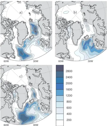
Figure 8. Surface topography and sea ice. Isolines mark the topography at 500 m intervals. Ice covered regions are colored. Over the ocean,
dark gray with red outline indicates areas with perennial ice cover (15 % level) in more than 50 % of the model years. Light gray with dark blue-black outline indicates temporary ice cover in more than 50 % of the model years. (a) The surface topography in mPISM averaged over the full 30 kyr of LGM-mPISM, orange lines in the ocean mark perennial ice cover in LGM-mPISM-W, light blue lines mark temporary ice cover in LGM-mPISM-W (b) The LGM topography reconstruction provided by Lev Tarasov (Tarasov and Peltier, 2003; Tarasov et al., 2012). (c) The surface topography from the ICE-5G reconstruction of Peltier (2004) and sea ice from LGM-ICE-5G. The corresponding plot for PI-mPISM is shown in Fig. 3a.
fluxes (not shown). The higher topography over the Cana-dian Arctic Archipelago and Greenland cools these regions, and following from that the air over the Nordic seas and the Arctic Ocean.
The global mean precipitation in LGM-mPISM (Fig. 4) of 0.96 m yr−1 is 7 % lower than in PI-mPISM. This differ-ence is especially pronounced in the regions north of 45◦N, where the precipitation is reduced by 18 % to 0.54 m yr−1. The difference in precipitation between LGM-ICE-5G and PI-mPISM is larger (−11 % globally, and −31 % north of 45◦N) because of the lower temperature and the resulting
lower atmospheric moisture content.
3.6 The LGM ocean
In LGM-mPISM, the NADW is formed southeast of Ice-land (Fig. 5b). The NADW cell of the overturning circulation peaks at 22.1 Sv (PI-mPISM: 17.0 Sv) at 32.5◦N at a depth of 1020 m. The NADW cell reaches approximately 65◦N. In contrast to PI-mPISM, hardly any deep water is formed in the Nordic seas or in the Labrador Sea. This is indicated by the March mixed layer depth in Fig. 5b. Because of the lack of NADW formation in the Nordic seas, the NADW cell does not extend north of the Greenland–Scotland Ridge. The strengthening of the NADW cell is in agreement with the re-sults of Lippold et al. (2012). Our model does not capture the shoaling of the AMOC generally found in proxies (Lynch-Stieglitz et al., 2007; Lippold et al., 2012). The AABW cell strengthens and peaks at 3.6 Sv at 21.5◦S and a depth of 3570 m.
In the LGM-ICE-5G experiment, the NADW cell is weaker than in LGM-mPISM. The stream function peaks at 18 Sv at 35.5◦N and a depth of 1020 m. The NADW cell is
a)
b)
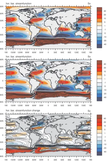
c)
Figure 9. Barotropic stream function. Positive values indicate
clockwise flow. (a) PI-mPISM, (b) LGM-mPISM, (c) LGM-ICE-5G – LGM-mPISM (a, b) For values beyond ±40 Sv, black contour lines are drawn at multiples of 20 Sv. (c) black con-tour lines show the circulation in LGM-mPISM at levels of ±1,5,10,20,40,60, . . .Sv. Dashed contour lines mark negative values.
The differences in ocean circulation can also be seen in the Atlantic ocean heat transport. In LGM-mPISM it reaches 1.1 PW at 23◦N (0.86 PW in PI-mPISM, 1.0 PW in LGM-ICE-5G). Between 15◦S and 35◦N, the overturning com-ponent dominates the heat transport and the differences be-tween the experiments (Fig. 10). It is highest in LGM-mPISM, where the overturning is strongest. In both LGM experiments in the Atlantic south of 35◦N the northward
At-lantic heat transport is stronger than in PI-mPISM. This ex-plains the simulated low cooling or even slight warming in the North Atlantic. Outside of this latitude band, the gyre transports become more important. Between 40 and 60◦N, the strong Subpolar Gyre dominates the transports in PI-mPISM and LGM-ICE-5G, while in LGM-PI-mPISM, the Sub-polar Gyre is weak and the overturning contributes
signifi-20 0 20 40 60 80
Latitude in °N 0.2
0.0 0.2 0.4 0.6 0.8 1.0 1.2
Northward heat transport in PW
LGM-mPISM
LGM-ICE-5G
PI-mPISM
Figure 10. Atlantic Ocean heat transports. Solid lines mark the total
heat transport, dashed lines the gyre contribution. The difference is the overturning contribution.
cantly. All experiments show similar total heat transports in the North Atlantic.
The sea ice in LGM-mPISM reaches further south in the North Atlantic than in PI-mPISM (see Figs. 3 and 8). It reaches Iceland during the entire year and covers large parts of the deep water formation areas of PI-mPISM. The win-ter sea ice margin reaches 63◦N east of Iceland and 43◦N at the American east coast. A part of the Labrador Sea be-comes ice-free during summer. In LGM-ICE-5G, the winter sea ice is similar to that of LGM-mPISM. The summer sea ice margin shifts to the north, the Norwegian Sea becomes ice-free and the summer sea ice cover in the Labrador Sea de-creases (Fig. 8). The reduced summer sea ice cover in LGM-ICE-5G is a combined effect of the missing latent heat flux from glacier melt (see below), and higher wind stress push-ing more ice out of the Labrador Sea.
Table 5. Heat budget of the Arctic Ocean sea ice in years 1650–
2349 of LGM-mPISM and the same years of LGM-mPISM-W (the comparison experiment with cut ice shelf–ocean heat fluxes). The boundary between the Arctic Ocean and the Nordic seas is drawn at the Fram Strait.
Flux LGM-
LGM-mPISM mPISM-W
Heat flux from the atmosphere (TW) −29.4 −38.3 Input from ice shelves
−12.3 0
(including calving) (TW)
Heat flux from the ocean (TW) 8.3 10.3 Heat export corresponding
to sea ice export (TW) 33.4 27.9
3.7 The LGM ice sheets
The total modeled land ice volume in the Northern Hemi-sphere is 60 Mio km3, corresponding to 150 m of sea level change. Table 6 lists the ice sheet volumes, Fig. 6 shows the time evolution of the volumes, and the mask used for this analysis. We compare our results to four reconstructions. The widely used ICE-5G reconstruction (Fig. 8c, Peltier, 2004), its follow-up ICE-6G as provided by the PMIP-3 project (PMIP3 Project members, 2010), the latest reconstruction by Lev Tarasov (Fig. 8b, Tarasov and Peltier, 2003; Tarasov et al., 2012, labeled as Tarasov in the following) and the re-construction by Kurt Lambeck as provided by the PMIP-3 project (PMIP3 Project members, 2010, ANU in the follow-ing). ICE-5G consists of a high-resolution bedrock topog-raphy combined with a coarse resolution ice thickness. The surface therefore is not smoothed out by the ice and much rougher than a real ice sheet surface. Local surface eleva-tions can therefore not be considered for comparisons. We therefore refer to the Tarasov reconstruction for small-scale features.
3.7.1 The LGM Greenland Ice Sheet
Of the 60 Mio km3 Northern Hemisphere ice volume, the Greenland Ice Sheet contains 5.8 Mio km3 (14.5 m SLE), compared to 4.3 Mio km3(10.8 m SLE) in the ICE-5G recon-struction (Peltier, 2004). It shows a drift of −2.7 km3yr−1 averaged over the full 30 kyr. The Greenland Ice Sheet’s two-dome structure closely resembles that in PI-mPISM. It is wider in all directions than in PI-mPISM, and covers all the continental slopes. The height of the northern dome is at 3150 m (100 m lower than in PI-mPISM, Tarasov: 3112 m). The southern dome profits from the cold climate and the wider ice sheet, and reaches a height of 2850 m (150 m higher than in PI-mPISM, Tarasov: 3083 m). The ICE-5G as well as the Tarasov reconstruction show a wider and flatter Green-land Ice Sheet during the LGM than the present GreenGreen-land Ice Sheet, but assume less ice at the margins than mPISM.
Table 6. LGM Ice sheet volumes and drift. For the time evolution
in the model, see Fig. 6. For the ICE-5G reconstruction, see Peltier (2004).
Volume (Mio km3) Drift(km3yr−1)
Ice sheet ICE-5G mPISM mPISM
Greenland 4.3 5.8 −2.6
Iceland 0.17 0.28 +1.2
Laurentide 36 31 +28
Siberia 0 9.3 +108
Fennoscandian 8.2 11.6 +156
Total 48.7 60 +233
In LGM-mPISM, the annual accumulation on the Green-land Ice Sheet of 558 Gt yr−1is exclusively balanced by di-rect losses to the ocean. Melting is negligible because of the lower surface temperatures. Figure 1 provides an overview of the ice streams. In the following, capital letters refer to the figure. The Northeast Greenland Ice Stream (A) surges re-peatedly. Its southern neighbor in a trough off Kejser Franz Joseph Fjord (B) shows similar surge-type behavior and matches deposits described by Wilken and Mienert (2006). South of it, at Scoresby Sund (C), an ice stream is contin-uously active matching glacial deposits found in this area (Wilken and Mienert, 2006). In the area of Kangerdlugssuaq Glacier (D) an ice stream continuously drains into the At-lantic. Further continuously active glaciers follow on the southern east coast. On the west coast, ice streams surge repeatedly in the region of Jakobshaven Isbrae (E) and the trough north of it, matching proxy observations in Roberts et al. (2009). Further north, in the region of Kong Oscar Glacier (F), two tributaries show surge-type activity. Since the sediment mask we use in mPISM (see Sect. 2.2) does not allow for sliding in the interior of Greenland (blue ar-eas in Fig. 1), the ice streams are limited to the continental shelf. This does not prohibit fast-flowing ice as in PI-mPISM (Fig. 7), where fast ice flow occurs in parts of the Green-land Ice Sheet where the sediment mask prohibits sliding. This fast flow is caused entirely by internal deformation. The inclusion of temperate ice in PISM allows for a very low vis-cosity, so the ice can reach high speeds by pure internal de-formation.
3.7.2 The LGM Laurentide Ice Sheet
The southern boundary is approximately at 50◦N in the west
and at 45◦N in the east.
The Laurentide Ice Sheet is split into a main part and a western Cordilleran part by the Mackenzie Ice Stream. This ice stream cuts down to below 1500 m a.s.l. and is in con-tinuous operation with an average strength of 694 Gt yr−1 (21 mSv water equivalent). During most of the experiment, Mackenzie Ice Stream shows net surface melt in its northern part because of a foehn-effect acting on the winds from the Pacific. This area is characterized by very low surface ele-vations. The main part of the Laurentide Ice Sheet has two domes that are separated by the Hudson Bay. The maximum height of the eastern dome is 3200 m (3600 m of ice thick-ness), the maximum height of the western dome is 3150 m (also 3600 m of ice thickness). The Hudson Bay area is largely drained by the Hudson Strait Ice Stream that approx-imately every 7000 yr flushes ice into the Labrador Sea. Un-less otherwise noted, we average over this oscillation in this chapter. Details of the oscillation and its implications in the climate system will be covered in a follow-up publication. They basically follow the binge–purge oscillator mechanism proposed by MacAyeal (1993) and first shown to work in 3-D by Calov et al. (2002). The main part of the Laurentide Ice Sheet loses ice by surface melt at its southern boundary and by calving into the ocean at the eastern and northern bound-aries.
The Cordilleran part of the Laurentide Ice Sheet reaches heights of up to 3550 m, but these elevations are reached only on high mountains, so the thickness there is about 1000 m. In valleys, the thickness reaches up to 2700 m, with surface heights of up to 2800 m. The surface accumulation of the Cordilleran part of the Laurentide Ice Sheet is balanced by the Mackenzie Ice Stream on the eastern side and by surface melt on the western side. The melt on the western side is pos-sible because of the high temperatures in the northern Pacific that locally exceed those in PI-mPISM. The modeled ice-free western coast could be a resolution artifact. The coarse reso-lution of the ISM could lead to an underestimation of the ex-tent of the ice streams. The coarse resolution of the AGCM is responsible for an underestimation of the strength of the pre-cipitation on the slope. On the other hand, the AGCM over-estimates the width of this belt of strong precipitation. The Cordilleran part of the Laurentide Ice Sheet covers Alaska fully. This is likely related to the same biases that cause the glaciation of the Alaska Range in PI-mPISM.
None of the reconstructions show an ice-free American west coast. They differ in the southern boundary and in the details of the structure of the interior of the ice sheet. All four reconstructions agree with our model in putting the south-western edge further to the north than the eastern edge, with values for the southwestern edge between 42◦N (ANU and ICE-6G) and 50◦N (Tarasov) (50◦N in our model). For the southeastern edge the values are between 35◦N (ANU and ICE-6G) and 40◦N (Tarasov and ICE-5G), while our model yields 45◦N. Considering that our climate model has a
reso-lution of about 3.75◦, this match is acceptable. In the ANU
reconstruction and in our model the Mackenzie Ice Stream splits the Laurentide Ice Sheet into a western and an east-ern part. In ICE-5G and in the Tarasov reconstruction this ice stream is less well represented. It is hardly discernible in ICE-6G. In the central part, the ANU reconstruction shows a higher surface elevation than our model, but the structure is very similar with a rather low surface elevation in the region of the Hudson Bay and higher surface elevation south and west of it. A similar structure can be seen in the Tarasov re-construction. West of the Hudson bay, ICE-5G, shows a mas-sive mountain range between 90◦W and 120◦W, reaching about 4500 m a.s.l.while ICE-6G has a peak in the Hudson Bay area.
A comparison of the ice streams simulated in the model (Fig. 1) with those found in proxy records (Stokes and Tarasov, 2010) shows several ice streams, where models and reconstructions agree. In the following, numbers relate to the numbering in Stokes and Tarasov (2010) and Fig. 1. The cen-tral Laurentide Ice Sheet is drained into the Arctic Ocean by Mackenzie Ice Stream (1). There are two major ice streams in the Canadian Arctic Archipelago, the Amundsen Gulf Ice Stream (18) just to the east of Mackenzie, and M’Clure Strait (19) north of Amundsen Gulf Ice Stream. Both show surge behavior. So does Lancaster Sound Ice Stream (22) with its tributaries, the Admirality Inlet (21) and the Gulf of Boothia ice stream (20). They drain the north-eastern part of the Lau-rentide Ice Sheet into Baffin Bay. Further to the south, hardly represented, the Cumberland Sound Ice Stream (23) surges into the Davis Strait. South of Cumberland Sound and well represented, the Hudson Strait Ice Stream (24) drains the Hudson Bay into the Labrador Sea. The Hudson Strait is not the only possible ice stream route for draining the Hudson Bay. The sediment distribution allows for a more northerly route joining the Lancaster Sound Ice Stream and draining into the northern corner of Baffin Bay. However, this route does not become active in our experiments (Fig. 1). A repeat-edly surging ice stream drains the Ungava Bay (16) into the Hudson Strait. In the Gulf of St Lawrence, a large ice stream system forms in the Laurentian Channel (25) and neighbor-ing tributaries.
3.7.3 The LGM Eurasian ice sheets
the West. Krinner et al. (2011) concluded that two impor-tant factors for not glaciating eastern Siberia are (1) the low snow albedo that is caused by dust deposition, and (2) mois-ture blocking by the Fennoscandian Ice Sheet. We do not use a locally varying glacier albedo, so the first effect is not rep-resented in our setup. The modeled Fennoscandian Ice Sheet does not reach as far south as indicated by the reconstruc-tions and the coarse resolution of the Atmosphere model does not allow for a realistic simulation of the moisture block-ing. Furthermore, we run the model under LGM boundary conditions for a long time span, so our (steady-state) re-sponse must be expected to be different from a transient state (see Sect. 3.7.4). The East Siberian Ice Sheet loses mass by surface melt along all margins except for the Arctic Ocean coast, where the losses occur by calving and shelf basal melt only. Further calving and shelf basal melt occur at the Pacific coast.
The Fennoscandian Ice Sheet has a volume of 11.6 Mio km3 (29.2 m SLE; ICE-5G: 8.2 Mio km3, 20.7 m SLE) and shows a drift of+156 km3yr−1. It consists of two main parts. One part covers the Barents, Kara and Laptev sea shelves and the islands in this region up to Svalbard in the northwestern corner. The other part covers Scandinavia south to 60◦N. The eastern part starts with a peak height of 2600 m. During the experiment, the ice sheet expands southward, and the peak shifts to the south and grows to 3000 m. The western part starts with a peak height of 2730 m, decreases to 2600 m during the first 10 000 yr, and then stabilizes. Along the southern border and parts of the Norwegian Sea coast, there is surface melt. At the Arctic Ocean coast, all losses occur directly into the ocean.
Among the reconstructions of the Fennoscandian Ice Sheet, ICE-5G and ICE-6G show the largest low-thickness zones. Such zones are hard to obtain as a steady-state so-lution in a dynamical ISM, where there are positive feed-backs for ice sheet growth, until either height desertification or a nearby coast limit the ice sheet height. They are easier to obtain as a transient state. The closure of the gap between the Fennoscandian Ice Sheet and the East Siberian Ice Sheet at the end of the coupled experiment shows such a large, flat zone that is growing by surface accumulation. ICE-5G por-trays the Fennoscandian Ice Sheet as reaching far to the south and staying below 1000 m in its southern parts. In the ANU reconstruction, the region between 50 and 60◦N is covered with substantially thicker ice exceeding 1500 m in large parts and even exceeding 2500 m over Norway. The surface eleva-tions in the Tarasov reconstruction are lower over Norway and the Barents Sea than in the ANU reconstruction, but the reconstructions largely agree. Over the Barents, Kara, and Laptev seas, our model places much more ice than any of the reconstructions. There are massive ice streams between Norway and Svalbard (α), and further streams between the present-day islands at the northern margin of the ice sheet (β, γ). They match with proxy records (Denton and Hughes,
1981). The southern margin ice streams cannot be compared to the reconstructions, since the margin is too far to the north. Iceland is covered by an ice cap with a volume of 278 000 km3 (0.7 m SLE, ICE-5G: 172 000 km3, or 0.43 m SLE) and a maximum height of 2450 m (1400 m ice thick-ness).
3.7.4 Long-term ice sheet changes
Figure 6 shows the evolution of the ice sheet volumes in LGM-mPISM. The largest changes occur on the Bering Sea shelf and between the East Siberian and Fennoscandian ice sheets. The Bering Sea shelf is flooded with ice from Alaska between years 9000 and 11 000. The ice stream surges trans-port vast amounts of ice into the region (Fig. 1) and, in the first years, have to compensate for strong surface melt. Over time, the ice sheet stabilizes.
The eastern part of the Fennoscandian Ice Sheet slowly expands southward. This allows the ridge to shift southward and increase in altitude. For the first 20 000 ice model years, the snow in the region between the Fennoscandian and the Siberian ice sheets melts during the summer, except for a few cold years, when it survives the summer melt. The ice sheets slowly grow into this area by lateral ice advection and start closing the gap from the sides. During the last 10 kyr, the winter snow in the gap between the ice sheets survives the summer melt, and the gap between the ice sheets is closed by glacier growth from local accumulation.
The simulated extensive glaciation of northern Siberia is likely to be an artifact of prescribing constant LGM bound-ary conditions. In the coupled ice–climate simulations of Heinemann et al. (2014), a transient simulation starting at 80 kyr BP shows a rather small LGM Fennoscandian Ice Sheet, while a steady-state simulation branched off from this LGM state grows a massive ice sheet covering most of Siberia. The steady-state Laurentide and Greenland ice sheets were very similar to the transient versions. This shows that the Fennoscandian Ice Sheet is far from equilibrium at the LGM. Another factor that prevented the growth of an ice sheet in Siberia is the reduction in the snow surface albedo by increased dust deposition during the last glacial (Krinner et al., 2011). This effect led to increased temperatures and melt in Siberia. It is likely that the model’s cold bias over northern Siberia for the present day could lead to a similar cold bias in the LGM simulations. This could additionally contribute to the growth of the Siberian Ice Sheet.
4 Summary and conclusions
AOVGCM ECHAM5/ MPIOM/ LPJ. Both models, as well as the coupling, work without anomaly maps or flux correction. This avoids inconsistencies between flux correction terms and modeled climate changes. In comparison to simulations using EMICs, AOGCMs represent processes of the ocean cir-culation and atmosphere dynamics in a much more detailed way and with higher spatial and temporal resolution. In con-trast to previous AOGCM–ISM simulations (e.g., Gregory et al., 2012), the ISM covers all relevant parts of the North-ern Hemisphere. mPISM is a SIA–SSA hybrid model, and is thus able to model ice streams more realistically than conven-tional SIA-only ISMs. The ISM is bidirecconven-tionally coupled to the atmosphere as well as to the ocean model, enabling the study of the full interactions between the ice sheets and the climate system.
We validated our setup by performing steady-state ex-periments under pre-industrial boundary conditions (PI-mPISM). The results agree reasonably well with the observational data. The global mean SAT in PI-mPISM is below that of ERA-INTERIM, representing the lower pre-industrial greenhouse gas concentrations. The NADW cell strength agrees with the estimates obtained from observa-tions. The NADW is formed in the Nordic and Labrador seas. In PI-mPISM, an ice sheet in the Alaska Range forms. This is due to a resolution-dependent cold bias in the atmosphere model in an area characterized by individual glaciers and ice fields.
With the same setup, we performed the first fully coupled multi-millennial steady-state AOVGCM–ISM simulations under LGM boundary conditions (LGM-mPISM). Again, the results agree reasonably well with proxy data. The NADW formation shifts to southeast of Iceland. The heat fluxes from ice shelf basal melt and calving contribute 30 % of the cool-ing of the Arctic Ocean. Cuttcool-ing them leads to thinncool-ing of the sea ice cover and an increase in the ocean–atmosphere heat flux, as well as to a reduction in the summer sea ice cover in the Nordic and Labrador seas.
During the long steady-state LGM simulations, a spuri-ous ice sheet forms in eastern Siberia and Alaska. This is at least partly due to neglecting the albedo effect of dust on snow and ice in our model, which would increase surface ab-lation in this region and probably prevent ice sheet growth (Warren and Wiscombe, 1980; Krinner et al., 2011). Further advances could be made by using a sophisticated energy bal-ance scheme for the surface mass balbal-ance (e.g., Calov et al., 2005; Vizcaíno, 2006) and a higher model resolution that can resolve the small-scale features of the glaciation in these re-gions. Finally, LGM-mPISM is a multi-millennial integra-tion under constant LGM boundary condiintegra-tions, while the LGM in reality was a transient state, where the ice sheets and the climate were not in an equilibrium. The ice sheet in Siberia might in part simply be the result of running the model too long under LGM boundary conditions. Modeling the last glacial as a transient process in AOGCMs is a major challenge for the years to come.
When the model is forced with the ICE-5G ice sheet recon-struction, the LGM cooling is stronger than in LGM-mPISM. In contrast to LGM-mPISM, the NADW is largely formed in the Labrador Sea. It is possible to switch between the deep water formation regions of LGM-mPISM and LGM-ICE-5G by exchanging the ice sheets. This provides a mechanism for obtaining two different ocean circulation states in glacial cli-mate simulations.
mPISM shows strong surge behavior in the Hudson Strait, as well as in several other regions. These surges follow the Heinrich event mechanism described by MacAyeal (1993) and first modeled in 3-D by Calov et al. (2002). The response of the climate system shows the basic features of Heinrich events (Heinrich, 1988; Clement and Peterson, 2008). We currently study the effects of a transient spinup and the pro-cesses relevant for the last deglaciation with the coupled model system.
Acknowledgements. This work was supported by the Max Planck Society for the Advancement of Science and the International Max Planck Research School on Earth System Modelling. Computa-tional resources were made available by the German Climate Com-puting Center (DKRZ) through support from the German Federal Ministry of Education and Research (BMBF).
Special thanks to Ed Bueler and the PISM group at the University of Alaska, Fairbanks, for providing their model and great support for its use. Development of PISM is supported by NASA grants NNX13AM16G and NNX13AK27G.
ERA INTERIM (Dee et al., 2011) climate reanalysis data was provided by the European Centre for midrange weather forecasts (ECMWF).
Precipitation data from the GPCP project was obtained through the integrated climate data center of the KlimaCampus Hamburg. The GPCP combined precipitation data were developed and com-puted by the NASA/Goddard Space Flight Center’s Laboratory for Atmospheres as a contribution to the GEWEX Global Precipitation Climatology Project.
Edited by: V. Rath
The service charges for this open access publication have been covered by the Max Planck Society.
References
Abe-Ouchi, A., Segawa, T., and Saito, F.: Climatic Conditions for modelling the Northern Hemisphere ice sheets throughout the ice age cycle, Climate of the Past, 3, 423–438, doi:10.5194/cp-3-423-2007, 2007.
Abe-Ouchi, A., Saito, F., Kawamura, K., Raymo, M. E., Okuno, J., Takahashi, K., and Blatter, H.: Insolation-driven 100,000-year glacial cycles and hysteresis of ice-sheet volume, Nature, 500, 190–193, 2013.
Project (GPCP) Monthly Precipitation Analysis (1979– Present), J. Hydrometeor., 4, 1147–1167, doi:10.1175/1525-7541(2003)004<1147:TVGPCP>2.0.CO;2, 2003.
Amante, C. and Eakins, B. W.: ETOPO1 1 Arc-Minute Global Re-lief Model: Procedures, Data Sources and Analysis, Tech. rep., NOAA Technical Memorandum NESDIS NGDC-24, 2009. Annan, J. D. and Hargreaves, J. C.: A new global reconstruction of
temperature changes at the Last Glacial Maximum, Clim. Past, 9, 367–376, doi:10.5194/cp-9-367-2013, 2013.
Arpe, K., Leroy, S. A. G., and Mikolajewicz, U.: A compari-son of climate simulations for the last glacial maximum with three different versions of the ECHAM model and implica-tions for summer-green tree refugia, Clim. Past, 7, 91–114, doi:10.5194/cp-7-91-2011, 2011.
Aschwanden, A., Bueler, E., Khroulev, C., and Blatter, H.: An en-thalpy formulation for glaciers and ice sheets, J. Glaciol., 58, 441–457, doi:10.3189/2012JoG11J088, 2012.
Bamber, J. L., Layberry, R. L., and Gogineni, S. P.: A new ice thick-ness and bed data set for the Greenland ice sheet 1. Measurement, data reduction, and errors, J. Geophys. Res., 106, 33773–33780, doi:10.1029/2001JD900054, 2001.
Barr, I. D. and Clark, C. D.: Late Quaternary glaciations in Far NE Russia; combining moraines, topography and chronology to as-sess regional and global glaciation synchrony, Quat. Sci. Rev., 53, 72–87, doi:10.1016/j.quascirev.2012.08.004, 2012.
Bigg, G. R., Clark, C. D., and Hughes, A. L. C.: A last glacial ice sheet on the Pacific Russian coast and catastrophic change arising from coupled ice–volcanic interaction, Earth Planet. Sci. Lett., 265, 559–570, doi:10.1016/j.epsl.2007.10.052, 2008.
Bonelli, S., Charbit, S., Kageyama, M., Woillez, M.-N., Ramstein, G., Dumas, C., and Quiquet, A.: Investigating the evolution of major Northern Hemisphere ice sheets during the last glacial-interglacial cycle, Clim. Past, 5, 329–345, doi:10.5194/cp-5-329-2009, 2009.
Box, J. E., Bromwich, D. H., Veenhuis, B. A., Bai, L.-S., Stroeve, J. C., Rogers, J. C., Steffen, K., Haran, T., and Wang, S.-H.: Greenland Ice Sheet Surface Mass Balance Variability (1988– 2004) from Calibrated Polar MM5 Output, J. Climate, 19, 2783– 2800, doi:10.1175/JCLI3738.1, 2006.
Braconnot, P., Otto-Bliesner, B., Harrison, S., Joussaume, S., Pe-terchmitt, J.-Y., Abe-Ouchi, A., Crucifix, M., Driesschaert, E., Fichefet, Th., Hewitt, C. D., Kageyama, M., Kitoh, A., Laîné, A., Loutre, M.-F., Marti, O., Merkel, U., Ramstein, G., Valdes, P., Weber, S. L., Yu, Y., and Zhao, Y.: Results of PMIP2 coupled simulations of the Mid-Holocene and Last Glacial Maximum – Part 1: experiments and large-scale features, Clim. Past, 3, 261– 277, doi:10.5194/cp-3-261-2007, 2007.
Braconnot, P., Harrison, S. P., Otto-Bliesner, B. L., Abe-Ouchi, A., Jungclaus, J. H., and Peterschmitt, J.-Y.: The Paleoclimate Mod-eling Intercomparison Project contribution to CMIP5, CLIVAR Exchanges, 56, 15–19, 2011.
Braconnot, P., Harrison, S. P., Kageyama, M., Bartlein, P. J., Masson-Delmotte, V., Abe-Ouchi, A., Otto-Bliesner, B., and Zhao, Y.: Evaluation of climate models using palaeoclimatic data, Nature Clim. Change, 2, 417–424, doi:10.1038/nclimate1456, 2012.
Braithwaite, R. J. and Olesen, O. B.: Glacier fluctuations and cli-matic change, 219–233, Kluwer, 1989.
Bryan, F. O., Hecht, M. W., and Smith, R. D.: Resolution con-vergence and sensitivity studies with North Atlantic circulation models. Part I: The western boundary current system, Ocean Modell., 16, 141–159, doi:10.1016/j.ocemod.2006.08.005, 2007. Budd, W. F. and Smith, I. N.: The growth and retreat of ice sheets in response to orbital radiation changes, in: Proceedings of the Canberra Symposium, December 1979, no. 131 in IAHS Publ., 369–409, 1979.
Bueler, E. and Brown, J.: Shallow shelf approximation as a sliding law in a thermomechanically coupled ice sheet model, J. Geo-phys. Res., 114, F03008, doi:10.1029/2008JF001179, 2009. Calov, R. and Greve, R.: A semi-analytical solution for the
posi-tive degree-day model with stochastic temperature variations, J. Glaciol., 51, 173–175, 2005.
Calov, R., Ganopolski, A., Petoukhov, V., Claussen, M., and Greve, R.: Large-scale instabilities of the Laurentide ice sheet simulated in a fully coupled climate-system model, Geophys. Res. Lett., 29, 691–694, doi:10.1029/2002GL016078, 2002.
Calov, R., Ganopolski, A., Claussen, M., Petoukhov, V., and Greve, R.: Transient simulation of the last glacial inception. Part I: glacial inception as a bifurcation in the climate system, Clim. Dynam., 24, 545–561, doi:10.1007/s00382-005-0007-6, 2005. Charbit, S., Ritz, C., Philippon, G., Peyaud, V., and Kageyama,
M.: Numerical reconstructions of the Northern Hemisphere ice sheets through the last glacial-interglacial cycle, Clim. Past, 3, 15–37, doi:10.5194/cp-3-15-2007, 2007.
Clark, P. U., Dyke, A. S., Shakun, J. D., Carlson, A. E., Clark, J., Wohlfarth, B., Mitrovica, J. X., Hostetler, S. W., and Mc-Cabe, A. M.: The Last Glacial Maximum, Science, 325, 710– 714, doi:10.1126/science.1172873, 2009.
Clement, A. C. and Peterson, L. C.: Mechanisms of abrupt climate change of the last glacial period, Rev. Geophys., 46, RG4002, doi:10.1029/2006RG000204, 2008.
Dee, D. P., Uppala, S. M., Simmons, A. J., Berrisford, P., Poli, P., Kobayashi, S., Andrae, U., Balmaseda, M. A., Balsamo, G., Bauer, P., Bechtold, P., Beljaars, A. C. M., van de Berg, L., Bid-lot, J., Bormann, N., Delsol, C., Dragani, R., Fuentes, M., Geer, A. J., Haimberger, L., Healy, S. B., Hersbach, H., Hólm, E. V., Isaksen, L., Kå llberg, P., Köhler, M., Matricardi, M., McNally, A. P., Monge-Sanz, B. M., Morcrette, J.-J., Park, B.-K., Peubey, C., de Rosnay, P., Tavolato, C., Thépaut, J.-N., and Vitart, F.: The ERA-Interim reanalysis: configuration and performance of the data assimilation system, Quart. J. Roy. Meteorol. Soc., 137, 553–597, doi:10.1002/qj.828, 2011.
Denton, G. H. and Hughes, T. J.: The Last Great Ice Sheets, Vol. 1, Wiley, 1981.
Ettema, J., van den Broeke, M. R., van Meijgaard, E., van de Berg, W. J., Bamber, J. L., Box, J. E., and Bales, R. C.: Higher surface mass balance of the Greenland ice sheet revealed by high-resolution climate modeling, Geophys. Res. Lett., 36, doi:10.1029/2009GL038110, 2009.
Fausto, R. S., Ahlstrø m, A. P., van As, D., and Steffen, K.: Present-day temperature standard deviation parameterization for Green-land, J. Glaciol., 57, 1181–1183, 2011.
Fettweis, X.: Reconstruction of the 1979–2006 Greenland ice sheet surface mass balance using the regional climate model MAR, The Cryosphere, 1, 21–40, doi:10.5194/tc-1-21-2007, 2007. Fichefet, T., Poncin, C., Goosse, H., Huybrechts, P., Janssens, I., and