ERICA CASTILHO RODRIGUES
INFERINDO A ESTRUTURA DE VIZINHANÇA EM
MODELOS BAYESIANOS ESPACIAIS
ERICA CASTILHO RODRIGUES Orientador: Renato Martins Assunção
INFERINDO A ESTRUTURA DE VIZINHANÇA EM
MODELOS BAYESIANOS ESPACIAIS
Dissertação apresentada ao Programa de Pós-Graduação em Estatística da Universidade Federal de Minas Gerais como requisito parcial para a obtenção do grau de Mestre em Estatís-tica.
ERICA CASTILHO RODRIGUES
ERICA CASTILHO RODRIGUES Advisor: Renato Martins Assunção
INFERINDO A ESTRUTURA DE VIZINHANÇA EM
MODELOS BAYESIANOS ESPACIAIS
Dissertation presented to the Graduate Pro-gram in Estatística of the Universidade Fed-eral de Minas Gerais in partial fulfillment of the requirements for the degree of Master in Estatística.
ERICA CASTILHO RODRIGUES
UNIVERSIDADE FEDERAL DE MINAS GERAIS
FOLHA DE APROVAÇÃO
Inferindo a estrutura de vizinhança em modelos bayesianos espaciais
ERICA CASTILHO RODRIGUES
Dissertação defendida e aprovada pela banca examinadora constituída por:
Ph. D.Renato Martins Assunção – Orientador Universidade Federal de Minas Gerais
Ph. D.Rosângela Helena Loschi Universidade Federal de Minas Gerais
Ph. D. Marc Genton Texas A&M University
Acknowledgments
Agradeço primeiramente a Deus, por me permitir terminar mais essa etapa.
Não poderia deixar de agradecer em primeiro lugar aos meus pais, Ricardo e Marcia. À minha mãe, pela paciência em me ouvir todos os dias, por participar em todos os momento, sempre me confortando e me incentivando. Ao meu pai, por sempre acreditar em mim, por sempre me ajudar em tudo que fosse possível. À Gabriela, pela compreensão e pela torcida sempre constante. Gostaria de agradecer também ao Taciano, pelo amor e incentivo incondicionais. Por sempre me ouvir, me dar conselhos e por sempre compartilhar comigo cada momento dessa jornada. Não posso também deixar de agradecer às minhas grandes amigas, Poliana, Natália e Sarah, pelos ótimos momentos compartilhados e por sempre torcerem por mim.
Resumo
No mapeamento de doenças, é necessário especificar uma estrutura de vizinhança para fazer inferências sobre a distribuição geográfica dos riscos relativos. Propomos um modelo em que a estrutura de vizinhança é parte do espaço paramétrico. Mantemos a propriedade de Markov usual de modelos Bayesianos espaciais: dado o grafo de vizinhança, as taxas de doença seguem um modelo auto-regressivo condicional. No entanto, o grafo em si é um parâmetro que também precisa ser estimado. Investigamos propriedades teóricas do nosso modelo. Em particular, investigamos cuidadosamente a matriz de covariância a priori e a
posteriori induzida por esta estrutura de vizinhança aleatória fornecendo interpretação para cada elemento dessas matrizes. Também ilustramos as vantagens do nosso modelo com os dados simulados e exemplos de mapeamento real da doença.
Palavras-chaves: Mapeamento de doenças; Campos Aleatórios de Markov; Modelos Hierárquicos Espaciais.
Abstract
In Bayesian disease mapping, one needs to specify a neighborhood structure to make inference on the underlying geographical relative risks. We propose a model in which the neighborhood structure is part of the parameter space. We retain the Markov property of the usual Bayesian spatial models: given the neighborhood graph, the disease rates follow a conditional autore-gressive model. However, the neighborhood graph itself is a parameter that also needs to be estimated. We investigate the theoretical properties of our model. In particular, we investi-gate carefully the prior and posterior covariance matrix induced by this random neighborhood structure providing interpretation for each element of these matrices. We also illustrate the advantages of our model with simulated data and real disease mapping examples.
Resumo Estendido
Em modelos espaciais e, mais especificamente, em modelos para mapeamento de doenças, um ponto importante é a especificação da estrutura de vizinhança. Apesar da importância dessa escolha, em geral, são utilizadas apenas relações de adjacência entre as áreas. Existem poucas justificativas para essa prática além da facilidade de implementação através de rotinas GIS. O nosso objetivo, portanto, é propor um modelo mais flexível, no qual a própria estrutura de vizinhança faz parte do espaço paramétrico. Ela será estimada e se adaptará de acordo com a estrutura espacial da base de dados que está sendo analisada.
Para tanto, utilizamos Campos Markovianos Gaussianos e mantemos a propriedade usual de Markov dos modelos espaciais. A nossa modificação é colocar uma matriz de precisão que apresenta uma forma mais genérica e que nos permite estimar o grafo de vizinhança. Ao invés de considerarmos apenas vizinhanças locais, incluímos a possibilidade de vizinhanças com alcances mais longos. Mostramos através de exemplos simulados e com dados reais, que em muitos casos a estrutura de vizinhança local pode não ser suficiente para captar toda informação espacial contida nos dados.
Esse trabalho está organizado da seguinte maneira.
No Capítulo 1, apresentamos a notação utilizada e o modelo proposto pelos autores. Mostramos que a matriz apresentada é, de fato, uma matriz de precisão de uma distribuição normal multivariada, visto que ela é definida positiva. Encontramos ainda as distribuições condicionais do efeito aleatório de uma área dado o resto do mapa e observamos que elas apresentam um apelo intuitivo. Finalmente, ainda nessa seção, reescrevemos a distribuição conjunta de uma maneira mais simples a fim de evidenciar mais uma forma de interpretá-la e mostrar que ela consiste, na verdade, em uma mistura geométrica de distribuições normais. No Capítulo 2, analisamos algumas propriedades teóricas do modelo. Em particular, estudamos cuidadosamente o formato das matrizes de covariância a priori e a posteriori
induzidas por essa vizinhança aleatória. Apresentamos uma interpretação de cada um de seus elementos e mostramos como eles refletem o tipo de estrutura especificada através da matriz de precisão. Além disso, para um melhor entendimento do modelo, consideramos um caso específico, no o qual a inversão das matrizes de covariância a priori e a posteriori são mais simples e a interpretação dos seus termos pode ser feita de maneira mais direta.
No Capítulo 3, ilustramos algumas vantagens do modelo por meio de dados simulados e exemplos com dados reais. O primeiro exemplo considerado se refere aos dados de mortal-idade infantil na cmortal-idade de Auckland. Nesse caso, notamos que a estrutura de vizinhança
mais razoável é aquela que considera todas as áreas como vizinhas umas das outras. Isso provavelmente se deve à homogeneidade da região analisada. O segundo exemplo analisado se refere à mortalidade causada por câncer pulmão, traquéia, brônquios e plêura. Novamente a estrutra de vizinhança estimada a posteriori foi aquela que considera todas as áreas vizinhas entre si. Para fins de comparação, consideramos uma terceira base de dados referente aos casos de mortes súbitas na infância. Calculamos algumas medidas de ajuste de modelos como DIC e o CPO e ambos mostraram que o nosso modelo apresenta resultados mais satisfatórios que os demais. Finalmente, geramos uma simulação de casos com risco constante e notamos que apesar de pontualmente todos os modelos darem a estimativa correta do risco relativo, nós fomos capazes de obter estimativas mais precisas.
Contents
1 Introduction 1
1.1 Motivation . . . 1
1.2 Disease Mapping . . . 3
2 Model 8 2.1 Model properties . . . 8
2.1.1 Posterior Covariance Matrix . . . 10
2.1.2 The specific case of two components . . . 12
3 Application and conclusion 13 3.1 Some illustrative applications . . . 13
3.1.1 Case study 1 . . . 13
3.1.2 Case study 2 . . . 14
3.1.3 Case study 3 . . . 18
3.1.4 Case study 4 . . . 19
3.1.5 Simulation . . . 21
3.2 Conclusions . . . 21
Bibliography 23
A Demonstration of result (2.4) 26 B Another interpretation for the terms (Si+S+j) 28
List of Figures
3.1 Map of SMR (left) and estimated relative risk (right) for Auckland data set. . . . 14
3.2 Posterior Densities of the parameters λ1, . . . , λ14 for the infant mortality rates in Auckland. . . 15
3.3 Map of SMR (above) and estimated relative risk (below). . . 16
3.4 Posterior Densities of λ’s. . . 17
3.5 Posterior Densities of λ’s for Sudden Death data set. . . 19
3.6 Posterior Densities of λ’s for Brazilian data. . . 20
List of Tables
3.1 DIC criterion for Auckland data base. . . 15
3.2 DIC criterion for Tennessee data base. . . 16
3.3 Summary measures of CPO considering Tennessee data set. . . 17
3.4 DIC criterion for North Carolina data base. . . 18
3.5 Summary measures of CPO considering North Carolina data set. . . 19
3.6 DIC criterion for Brazilian data base. . . 20
3.7 Summary measures of CPO considering Brazilian data set. . . 20
Chapter 1
Introduction
1.1
Motivation
In disease mapping, the Bayesian model proposed by Besag, York and Mollié (1991), and denoted by BYM, is the most popular choice to estimate relative risks in small areas or to evaluate the effects of covariates acting as exposure measurements surrogates. Originally, BYM was introduced to model a cross-section of counts collected in a set disjoint geograph-ical areas composing a partitioned map. Since then, BYM has been extended into several directions to include space-time generalized linear models (MacNab (2001), Beneito et al. (2008), Knorr-Held et al. (2001), Sun et al. (2000), Silva (2008)), spatial survival models (Carlin et al. (2003), Jin and Carlin (2005)), spatially-varying parameters models (Assunção et al. (2002), Assunção (2003), Gelfand et al. (2003)), and generalized additive models (Lan and Fahrmeir (2001)). Multivariate extensions incorporating two correlated sets of spatial effects have also been proposed in recent years Jin et al. (2005) , Gelfand and Vounatsou (2003), Held et al. (2005), Held et al. (2006). Many of these models can be fit using freely available software such as WinBUGS and BayesX.
BYM is based on a conditional autoregressive (CAR) model for the spatial random effects. In the CAR model, spatial dependence is expressed conditionally by requiring that the random effect in a given area, given the values in all other areas, depends only on a small set of neighboring values. More specifically, the random effect θi associated with the i-th area is
the sum φi+ψi of two components where φi is a spatially structured random effect assigned
an improper CAR prior distribution, and ψi is a second set of i.i.d. zero-mean normally
distributed unstructured random effects. This is termed a convolution prior (Besag, York and Mollie, 1991) since the density ofθi’s will be the convolution of the joint densities ofφi vector
and the ψi vector.
1. Introduction 2
Notwithstanding its crucial role in the spatial Bayesian models, very few studies have considered different neighborhood structures for disease mapping problems. One notable exception is MacNab and Dean (2000) where the authors considered a model for disease rates with spatial effects structured at two geographical levels. They used infant mortality data over the period 1985-1994 from the province of British Columbia (BC) in Canada. The areas were organized in 21 health units and their sub-divisions, 79 local health areas. Health units (HUs) are administrative health divisions overseeing the functioning of the health sub-units, the local health areas (LHAs). Therefore, it was natural to expect that LHAs within the same HUs should share many health service and care characteristics beyond those determined by factors that vary smoothly in space. Hence, they assumed a random effect shared by all LHAs within the same HU. They also considered a neighborhood structure in which two LHAs are considered neighbors if they share boundaries or if there is a third LHA sharing boundaries with both local health areas. This second-order neighborhood structure is less usual and it reminds the higher autoregressive order models in the time series setting.
A more recent reference is White and Ghosh(2009), who introduced a stochastic neighbor-hood CAR model where the selection of the neighborneighbor-hood depends on unknown parameters. They estimate how far should the neighborhood of the areas be assuming proximity weights that stay constant and equal to 1 up to a certain distance and thereafter decreases exponen-tially towards zero. In contrast with most of the published applied papers in disease mapping, they base their model in the proper CAR model rather than BYM. Most people prefer to use BYM, implying in an improper CAR model to deal with the spatial random effects, because the proper CAR model induces little marginal correlation between neighboring areas (See Banerjee, Carlin and Gelfand, 2004, page 81) and Assunção (2009).
These studies consider only locally larger neighborhoods than the first order neighborhood provided by the simple adjacency between the areas. Although in some situations a local neighborhood will be enough to deal with the spatial effects, we feel that spatial models should span a larger range of possibilities. Fundamentally, BYM and its variations consider the random effects being composed of either unstructured over-dispersion or small range spatial conditional variation. These are two extremes models and allowing for intermediate situations will be useful in some applications. We will show examples where the typical adjacency neighborhood structure is not sufficient to estimate the underlying risks, providing less smooth estimates than what should be inferred from the data. Our purpose is to introduce spatial effects with longer range than the immediate geographical neighborhood. This is likely to be useful specially in situations where the underlying risk changes so smoothly over larger regions as to be considered indistinguishable from a random constant value for all areas within it.
1. Introduction 3
also needs to be estimated. The methodology described herein permits arbitrary neighbor-hood extension for incorporating spatial random effects. It provides a simple mechanism for identifying the geographical extent of the conditional influence of neighboring areas.
The manuscript is organized as follows. In Section 1.2, we introduce the notation and present our model. In Section 2.1, we investigate the theoretical properties of the model. In particular, we carefully study the prior and posterior covariance matrix induced by this random neighborhood structure providing interpretation for each element of these matrices. We also present a specific and simpler case of our model allowing for a more thorough under-standing of the covariance structure. In Section 3.1, we illustrate the advantages of our model with simulated data and real disease mapping examples. We end in Section 3.2 presenting the main conclusions.
1.2
Disease Mapping
A Bayesian hierarchical model is one of the main tools to make inference on the underlying relative risks of a disease observed into disjoint geographical areas of a map. These models can be described in this way: suppose that we have N geographic areas and each of them has a relative riskψifori= 1, ..., N, that needs to be estimated. The Bayesian inference is based on
the posterior distribution of ψ = (ψ1, ..., ψN) given by f(ψ|y1, ..., yN) = l(y1, ..., yN|ψ)f(ψ),
where l(y1, ..., yN|ψ) is the likelihood function and f(ψ) is the prior distribution of the
pa-rameters vector ψ. Conditionally on the valuesψ1, ..., ψN, the valuesY1, ..., YN are supposed
to be independent with a Poisson distribution with meanψiEi, whereEi is the expected value
of cases under the hypotheses of constant relative risk over the areas. The modeling of the prior distribution f(ψ) allows the introduction of spatial dependence between the risks such that close regions tend to have similar relative risks. This dependence appears as a Markovian structure in which the value ψi of one area, conditionally on all other areas values, depends
only upon the ψj’s values of its neighbors.
More specifically, the relative risk ψi is written as
log(ψi) =µ+bi (1.1)
where µ is the general level of the relative risk and bi is the random effect of the i-th area.
One simple possibility is to assume that the random effects biare independent and identically
distributed with a normal distribution N(0, σ2). In this case, there will be no spatial effects imposed on the relative risks and the posterior distribution ofψwill reflect this independence. However, one typically anticipates a spatial dependence between the relative risks due to environmental and genetic similarities of neighboring areas. The most popular distribution to reflect the spatial structure of the data in the prior distribution was introduced by Besag et al (1991). They decomposed the random effect bi into two parts, a non-spatially-structured
component and a spatially structured component:
1. Introduction 4
where θ1, . . . , θn are the non-structured errors, independently and identically distributed
ac-cording to a normal distribution. The random effects βi have a spatially structured prior
distribution with intrinsic CAR (ICAR) distribution. The ICAR prior distribution is an im-proper prior with a Markovian structure. The distribution of βi, conditional on all the other
values βj for j̸=i, is given by
βi|β−i∼N (
¯
βi, σ2 ni
)
(1.2)
whereβ¯i is the mean of the i-th area neighboring values βj.
This model presents some identifiability problems of the spatial and non-spatial effects, as noticed by Eberly and Carlin(2000). To fix this problem, Leroux(1999) presented an alternative, including a parameter λ which is able to measure the effect of each component. This parameter measures the level of spatial correlation among the areas. In addition to this, it is included a parameter σ2 to measure the random effect variance. He proposed a multivariate normal distribution for the random effects b = (b1, . . . , bN) in (1.1) with the
following precision matrix
Q= (σ2)−1((1−λ)I+λR) (1.3)
whereIis the identity matrix andRis the precision matrix of the ICAR model, which means that
Rij =
ni if i=j
−1 if j∼j
0 otherwise
whereni is the number of neighbors of site iandi∼j means ineighbor ofj.
For this model, the parameter λ assumes values in the interval [0,1], anda hence, the precision matrix Q is a weighted sum of theI and Rmatrices.
The BYM and Leroux models represent a mixing of two extreme situations. One situation considers a conditional dependence only on the immediate neighbors represented by the single neighborhood structure while the other situation represents the complete independence be-tween the random effects. Both models consider that, if we have information on the immediate neighbors, no additional information about the other areas is necessary to make inference on the random effects. We think that in many practical situations this is too restrictive. Con-sider, for example, another extreme but possible situation in which the distribution ofbi (and
hence, of ψi) in a given area, conditional on the rest of the map, should depend upon all
the other sites, not only on the immediate neighbors. In this case, all areas are neighboring areas of all other areas. This can be a reasonable model when the region under study is small enough such that the economic, social and environmental characteristics are approximately constant over the entire region. This implies a certain exchangeability between the areas and therefore an all-inclusive dependence between the areas’ pairs. Every area gives incremental additional information on a fixed area value, even if conditioning on all the other areas.
1. Introduction 5
models to a larger class that has geographically increasing orders of neighborhood extension. Through Bayesian updating, we can make inference about the more appropriate neighborhood structure underlying the observed data. More specifically, we extend the weighted sum preci-sion matrix (1.3) by including matrices that represent neighborhoods of all possible orders in the simple adjacency graph.
Let each area i be a node or site of a graph and connect two nodes by one edge if they share boundaries. Let A be the n×nbinary adjacency matrix where Aij = 1if i andj are
connected by one edge, and Aij = 0otherwise. We say that iis a l-th order neighbor of j if
the (i, j)-th element of the power matrix Al is greater than zero and Asij = 0, for s < land
l≥1. The maximum neighborhood order is given by the diameter of the graph, which is the longest path among all the shortest paths that connect two sites. In other words, it counts the minimum number of steps necessary to leave a site and go to any other site in the graph. In our model, the vectorb = (b1, . . . , bN) in (1.1) has a multivariate normal distribution
with mean zero and precision matrix given by:
Q= (σ2)−1(λ1I+λ2R(1)+λ3R(2)+....+λk+1R(k) )
whereλ1+λ2+...+λk+1 = 1andλi≥0for alli. The integerkis the diameter of the graph
and R(l) is the graph Laplacian that includes neighborhoods up to order l. That is,
R(l)ij =
n(l)i if i=j
−1 ifj ∈∂i(l)
0 otherwise
where n(l)i is the number of neighbors of site i up to order l and ∂i(l) is the set of neighbors of area i, from order 1 up to order l. Notice that, we are considering that the neighborhood relationship is symmetric, that is, j∈∂i(l) if, and only if,i∈∂j(l). It is important to point out that these matrices are linearly independent, ensuring the parameters identifiability.
This matrix is positive definite, as it satisfies the sufficient condition of being diagonal dominant. That is, for all i= 1, . . . , n
Qii> N ∑
j=1
|Qij|
because
Qii=λ1+λ2n(2)i +λ3n (3)
i +...+λk+1n (k)
i =λ1+ N ∑
j=1
|Qij|> N ∑
j=1
|Qij|
asλ1 ∈(0,1), and, therefore, Q can be a precision matrix.
From the precision matrix, it is possible to obtain the conditional distribution bi|b−i of
1. Introduction 6
mean f(b, λ) and varianceg(b, λ) given by
f(b, λ) = λ2n
(1) i ¯b
(1)
i +λ3n(2)i ¯b (2)
i +. . .+λk+1n(k)i ¯b (k) i λ1+λ2n(1)i +λ3n
(2)
i +...+λk+1n (k) i
and
g(b, λ) = σ
2
λ1+λ2n(1)i +λ3n (2)
i +...+λk+1n (k) i
where ¯b(l)
i is the mean of neighbors of site i up to order l. The conditional expectation
is a convex linear combination of the means of its neighbors of all possible orders and the conditional variance is inversely proportional to the number of neighbors of each of these orders multiplied by their respective weight λl.
Let the(n−2)dimensionalb−ij be the vectorbwithout itsi−th andj−thcoordinates.
It can be shown that the conditional correlation between the areas, Corr(bi, bj|b−ij) is given
by
Corr(bi, bj|b−ij)∝
λ2+λ3+. . .+λk if j∈∂i(1) λ3+. . .+λk if j∈∂i(2)−∂
(1) i .
.
λk if j∈∂i(k)− ∪k−1
l=1 ∂ (l) i
.
with the proportionality constant given by the inverse of
k ∑
l=1
λln(l−1)i k ∑
l=1
λln(l−1)j
and with n(0)i ≡ 1 by definition, for all i = 1, . . . , N. This shows that the conditional correlation between the areas decreases with the neighborhood order l. For example, if a pair of sites are third order neighbors, the conditional correlation between them will be smaller than that between two first order neighbors. Notice also that, if all the λl are positive, then
1. Introduction 7
We can also write the joint distribution in a more interpretable way:
f(b) ∝ exp
− 1
2σ2
∑
i
b2i(λ1+...+λk+1n(ik))−λ2
∑
i
∑
j:j∈∂i(1)
bibj
−λ3
∑
i
∑
j:j∈∂(2)i
bibj−...−λk+1
∑
i
∑
j:j∈∂i(k)
bibj
= exp − 1
2σ2
λ1
∑
i
b2i +2λ2 2
∑
i
∑
j:j∈∂i(1)
b2i +. . .+2λk+1 2
∑
i
∑
j:j∈∂i(k)
b2i
−
2λ2
2
∑
i
∑
j:j∈∂i(1)
bibj+...+
2λk+1
2
∑
i
∑
j:j∈∂i(k)
bibj
= exp − 1
2σ2
∑ i
λ1b2i +
λ2
2
∑
j:j∈∂(1)i
(bi−bj)2+. . .+
λk+1
2
∑
j:j∈∂i(k)
(bi−bj)2
. (1.4)
Ifλl= 0for alll >1, we are in the case of independent normal distributions. We can interpret
the term associated with λl as a penalization for configurations showing too much variation
among l-th order neighbors. The larger the value of λl, the smoother is the spatial pattern
up to neighborhood order l.
This distribution can also be written as
f(b)∝
(
exp
{
− 1
2σ2 ∑
i b2i
})λ1
exp − 1
4σ2 ∑
i ∑
j:j∈∂i(l)
(bi−bj)2 λ2 ... exp − 1
4σ2 ∑
i ∑
j:j∈∂(il)
(bi−bj)2 λk
which is a geometric mixture of normal distributions.
To complete the model specification, one needs to adopt prior distributions for the weights
(λ1, . . . , λk) and for the hyperparameter σ2. In our applications, we assumed an inverse
Chapter 2
Model
2.1
Model properties
To gain a better understanding of the prior and posterior distribution properties, we obtain its marginal covariance matrix in addition to the conditional correlation given earlier. To avoid a cumbersome notation and long formulas, we will consider the model that includes three different values for λl, one corresponding toλ1 (associated with the individual areas and the
independent case), another corresponding to λ2 (associated with pairs of adjacent areas), and
the third one, λ3, corresponding to the highest possible order k, associated with a complete
graph, where every area is neighbor of every other area. The extension to the general case is straightforward.
Considering only three components, our precision matrix reduces to
Q= (σ2)−1(λ1I+λ2R(1)+λ3R(k) )
(2.1)
whereR(1) is the precision matrix of the ICAR model and R(k) is given by
R(k)=diag(N)−11T
where N = N1 with N being the total number of areas in the map and 1 denotes a N -dimensional vector of ones. The precision matrix in (2.1) can be rewritten as
Q= (σ2)−1(λ1I+λ2diag(n) +λ3diag(N)−λ2A−λ311T)
where Ais the binary adjacency matrix and A1=n= (n1, . . . , nN) is the vector which has
the number of adjacent neighbors of each area. From matrix algebra, we know that
(
P+uvT)−1 =P−1−P
−1uvTP−1
1 +vTP−1u (2.2)
if P is an invertible matrix and u and v are vectors with the same dimension. Let M =
2. Model 9
λ1I+λ2diag(n) +λ3diag(N)−λ2Aand denote by mij theij-th element of M−1. Using the
result (2.2), we have that the covariance matrix Q−1 is given by
Q−1 = σ2 (
M−1+λ3
M−111TM−1
1−λ31M−11T
)
= σ2M−1+ σ
2λ 3
1−λ3∑i,jmij ∑
jm1j∑imi1 ... ∑jm1j∑imiN .
. . ∑
jmN j∑imi1 ... ∑
jmN j∑imiN
As the matrix M is symmetric,M−1 is also symmetric and therefore, for alll= 1, ..., N,
∑
j
mlj = ∑
i mil.
Let Sl+=∑jmlj =∑imil. We can write the covariance matrix as
Q−1 =σ2M−1+ σ
2λ 3
1−λ3∑ijmij
[S1+ S2+. . . SN+]T [S1+ S2+ ... SN+] . (2.3)
To understand this covariance matrix, we consider initially the matrix M−1 by following the analytical approach adopted by Assunção and Krainski (2009). We can write
M−1 = M−1[λ1I+λ2diag(n) +λ3diag(N)] [λ1I+λ2diag(n) +λ3diag(N)]−1
= [I−λ2TA]−1T
where
T=diag
{
1
λ1+λ2n1+λ3N
, . . . , 1
λ1+λ2nN +λ3N }
. (2.4)
In the appendix, we show that we can expand the inverse matrix obtaining
[I−λ2TA]−1T=IT+λ2(TA)T+λ22(TA)2T+λ32(TA)3T+. . .
The elements [(TA)lT]ij of the the l-th matrix in this expansion are weighted sums of all possible paths of length l starting at the i-th site and ending at the j-th site. For example, the three first matrices have elements equal to
[(TA)T]ij = aij
(λ1+λ2ni+λ3N)(λ1+λ2nj +λ3N)
[
(TA)2T]ij =
N ∑
k=1
aikakj
2. Model 10
[
(TA)3T]ij =
N ∑ l=1 N ∑ k=1
aikaklalj
(λ1+λ2ni+λ3N)(λ1+λ2nk+λ3N)(λ1+λ2nl+λ3N)(λ1+λ2nj+λ3N) .
Considering the second matrix for illustration, the element [(TA)2T]
ij counts all paths i→ k → j giving a weight inversely proportional to the number of immediate neighbors ni,nk,
and nj the areas have. Going from i to j through a highly connected area has a smaller
contribution to M−1ij than if the path goes through a poorly connected intermediate area.
This shows that two areas in a region of the map with highly connected areas will tend to be less correlated than two areas in a region where the areas has few immediate neighbors. Isolated
To complete the understanding of the covariance matrix Q−1 in (2.3), we consider now
the valueSi+. We have
Si+ = N ∑ j=1 mij = N ∑ j=1 ∞ ∑ k=0
λk2[(TA)kT
] ij = ∞ ∑ k=0 λk2
N ∑
j=1 [
(TA)kT
]
ij .
where we interchange the order of the terms because the sum is absolutely convergent. This quantity is a weighted sum of all paths leaving site i, the weight decreasing with the path length k. It is inversely related to the average degree of connectivity that areaihas with the other areas in the graph. It is a value associated with the individual area, not with specific pairs of areas.
In summary, the covariance Cov(bi, bj) =Q−1ij is the sum of two components. The first one
is M−1ij and represents a weighted sum of all paths from ito j with weights inversely related to their length and to the connectivity of the areas in the path. The second component is given by the product ofSi+S+j whereSi+is a score associated with the average connectivity
of areaito the other areas in the map. The first component is influenced by the neighborhood structure through a weighted counting of each path from i to j. The second component is also influenced by the neighborhood structure but it considers only a marginal structure. Its presence in the covariance matrix position(i, j) is by means of the product of these marginal values associated with the individual areas.
2.1.1 Posterior Covariance Matrix
More relevant to the Bayesian data analysis is the posterior covariance implied by our prior spatial model. To obtain analytical expressions, assume that yi can be approximated by a
normal distribution with variance 1/τy. The posterior precision matrix is given by
Q∗ =τyI+Q=τy+ (
2. Model 11
and therefore, the covariance matrix is
Q∗−1 =M∗−1+
(
σ−2λ3)(M∗)−1(11T)(M∗)−1
1−(σ−2λ
3)1T (M∗)−11 .
where
M∗=
( τy+
λ1 σ2
)
I+ λ2
σ2diag(n) + λ3
σ2diag(N)− λ2 σ2A
It is rather surprising that it is possible to interpret each one of the two component matrices of the covariance Q∗−1. Considering initially (M∗)−1, after some algebraic manipulations
analogous to those carried out earlier for the prior covariance matrix, we have that
M∗−1 = [I−(τyλ3)T∗A]−1T∗
where
T∗ =diag
{
1
τy+σ−2(λ1+λ2n1+λ3N)
, . . . , 1
τy+σ−2(λ1+λ2nN +λ3N) }
.
The elements of this diagonal matrix involve the data precisionτy and the weights of the prior
covariance σ−2(λ1+λ2nN +λ3N). The relevance of each of these parts on the posterior
covariance will depend on the ratio between the variance of the observations and the prior variance.
The same matrix expansion that was used earlier can be applied here. Thus we have
M∗−1=T∗+(σ−2λ2)T∗AT∗+(σ−2λ2)2(T∗A) 2
T∗+(σ−2λ2)3(T∗A) 3
T∗+. . .
As a result, the posterior covariance matrix Q∗−1 has the same structure as the prior
covari-ance matrix, being written as sum of two matrices:
σ−2λ 3
1−σ−2λ
3∑i,jSij∗ ( S∗ 1+ )2 S∗
1+S2+∗ ... S1+∗ SN+∗ .
. . S∗
N+S1+∗ SN∗+S2+∗ ... ( S∗ N+ )2 and m∗
11 m∗12 ... m∗1N .
. . m∗
N1 m∗N2 ... m∗N N .
wherem∗
ij is the (i, j)-th element of the matrix M∗−1 and Sl+∗ = ∑
jm∗lj = ∑
im∗il
2. Model 12
possible paths between pairs of areas. While they were equal to (λ1+λ2ni+λ3N)−1 for
the prior, they are now equal to σ2/(τ
y +σ2(λ1+λ2ni+λ3N)). This means that, as the
prior covariance, the posterior covariance can be decomposed into two components reflecting different aspects of the neighborhood graph. One component is a weighted average of all paths connecting areasiandj, longer paths having smaller weights than shorter ones. Additionally, the paths are weighted according to the connection degree of the intervening areas in the path, more connected paths having less weights. The other component of [Q∗−1]ij reflects intrinsic
aspects of the pair of areas iand j. It does not matter where they are located with respect to each other, this covariance component is simply a product of scores specific to each area and, in this sense, has less spatial content than the first component.
2.1.2 The specific case of two components
We consider briefly a specific case in which the inversion of the prior and posterior covariance matrices are feasible and allow an easier interpretation of the covariance matrix. Suppose that, a priori, the area-specific valuesbi follows a multivariate normal distribution with mean
zero and precision matrix
Q= 1
σ2 (
(1−λ)I+λ(NI−11T)) .
whereλ∈(0,1). Compared with Leroux model in (1.3), this model exchanges the first order neighborhood matrix R of Leroux’s model by the matrix associated with the exchangeable risks model of Bernadinelli and Montomoli (1992).
Using (2.2), we can calculate the covariance matrix:
Q−1= σ
2
1−λ+λN
[
I+ λ
1−λ11
T ]
.
and the correlation Corr(bi, bj) = λ. The correlation approaches 1 as the weight of the
exchangeable model increases.
We can also find the posterior covariance matrix, if we assume that the data are normally distributed with variance(τy)−1. In this case, the posterior correlation of the random effects
of areas iandj is given by
Corr(bi, bj|y) =
λ
τy+ (σ2)−1(1−λ)
This correlation is close to zero if λ is also close to zero. In the opposite direction, to get correlation close to 1, we need to have λ close to 1 and also the ratio (σ2)τ
y between prior
Chapter 3
Application and conclusion
3.1
Some illustrative applications
In this section we will present some examples of application of our model and we will compare it whith ICAR and Leroux models.
3.1.1 Case study 1
Marshall(1990) studied the geographical variation of the infant (under 5 year of age) mor-tality in Auckland, New Zealand, for the period 1977-1985. Infant mormor-tality rates differed appreciably between developed countries between 1960 and 1990, with a typical decreasing trend. However, New Zealand and Sweden presented a different pattern with increasing rates, mostly due to the increase in the sudden death syndrome rates (see Mitchell, 1990). Figure 3.1 shows in the left hand side the mortality rates on 167 geographical units of the Auckland using the population of children under 5 years of age according to the 1981 census. In the right hand side is presented a map with the median of the rates estimated by our model, which is described in more details below. The global mean is 2.633 deaths per year per thou-sand but there is a large variation around this average level. The spatial pattern reflects the socioeconomic differences between the areas, with those less affluent with higher rates.
We fitted our model using the software WinBUGS to obtain the posterior distribution. If we take all possible neighborhood matrices R(l), we have l varying from 1 to 29. However, the higher order matrices are almost identical, varying by few entries from the previous order precision matrix. This shows that there will be little information to differentiate between them, which leads to severe identifiability problems. Therefore, we fit our model using the identity matrix, the neighborhood matrices up to order 11, and the matrix 11T full of ones.
We adopted a gamma distribution with parameters equal to 0.5 and 0.005 for the inverse of
σ2 and a uniform distribution on the 13-dimensional simplex for the weights (λ1, . . . , λ13).
This hyperprior distributions will be used in all the following examples.
The posterior distribution of theλlparameters is represented in the Figure 3.2. In the right
left hand side we show the estimated posterior density of λ1, the weight parameter associated
3. Application and conclusion 14
0.8 0.9 1.0 1.1 1.2 1.3 0.8 0.9 1.0 1.1 1.2 1.3
Figure 3.1: Map of SMR (left) and estimated relative risk (right) for Auckland data set.
hand side, we show all the other weights λ2, . . . , λ13. The matrix with the largest weight is
the identity, with the other neighborhood matrices receiving much smaller weights. In the right hand side, the density that stands out is that associated with the parameter λ13. This
means that the matrix 11T has a substantial weight if compared to the other neighborhood
matrices and it is likely due to the homogeneity of the region. In this example, the matrix associated with the exchangeable random effect component is more relevant in the estimation than the adjacency matrix, which is typically used in these analysis.
In order to compare the models, we calculated the DIC criterion for this model with 13 components (hereafter, called the K components model) and also for the Leroux and BYM models. From Table 3.1 we see that, in spite of the fact that this value for our model was a bit larger then the others, the three models compared are very similar in this regard.
To see if we can retain only the exchangeable component for this data set and throw away the spatial component, we also fit two specific cases of the general model. The first one is the model that was analyzed in Section 2.1 (three components) and is composed by the spatial and exchangeable matrices. The second one is the one analyzed in Section 2.1.2 (two components), which has only the exchangeable part. The results presented in Table 3.1 show that the DIC criterion is a bit larger for the model with only two components if compared with the model composed by three. This means that the spatial effect is relevant here. Even the results showing that the exchangeable component is the most important one, it is clear, from the map of SMR (Figure 3.1), that there is an spatial structure in this data set and this behavior was confirmed here comparing these two models.
3.1.2 Case study 2
tra-3. Application and conclusion 15
Table 3.1: DIC criterion for Auckland data base.
K components Two components Three components Leroux BYM
837.90 847.66 846.53 831.30 832.85
0.990 0.991 0.992 0.993 0.994
0
200
400
600
800
1000
1200
λ1
Density
0.000 0.002 0.004 0.006
0
5000
10000
15000
λ
Density
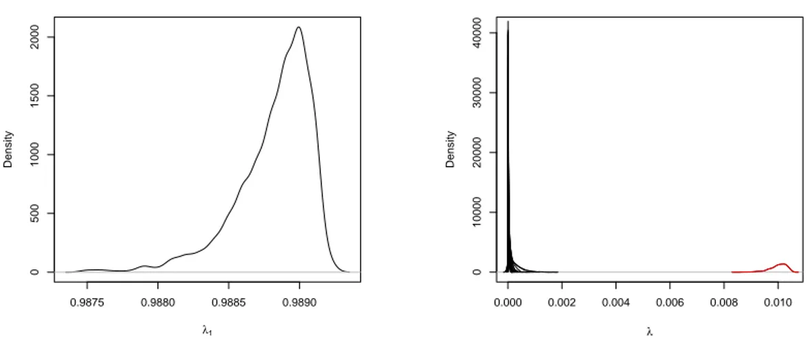
Figure 3.2: Posterior Densities of the parameters λ1, . . . , λ14 for the infant mortality rates in
Auckland.
chea, bronchus, and pleura cancers in the state of Tennessee. The period that was considered ranged from 1970 to 1994. It is well known that the changing in mortality patterns for this kind of cancer generally coincide with regional trends in cigarette smoking. Other studies have shown that the incidences rate is also related to occupational health hazard risks due to exposure to asbestos particles.
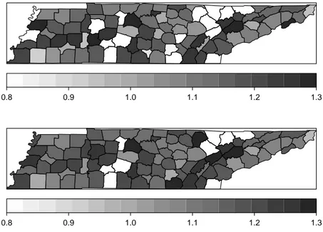
The map is divided into 95 counties and for each one of them we had the observed number of deaths as well as the expected number of deaths under the hypothesis of constant relative risk based on US rates. Figure 3.3 shows above the map with the relative risks estimated by the simple standardized mortality rate. Below it shows the estimates using our model. In this example, we are able to fit the model with all possible neighborhood matrices. Figure 3.4 presents the posterior densities of the weights. The graph on the left hand side shows that again the identity matrix is the most important. In the right hand side, we show density estimates of all remaining weights. The density that stands out is the weight associated with the matrix full of ones. Therefore, as happened with the previous example, a higher neighborhood order is required in the fit in order to estimate the underlying risks.
3. Application and conclusion 16
Table 3.2: DIC criterion for Tennessee data base.
K components Two components Three components Leroux BYM
868.813 864.63 864.70 860.44 858.80
and the two components models. We notice then that, although our model has shown a worse performance in relation to this criterion, the difference among them is small. An interesting fact to note here is that the DIC criterion for the model of three components does not differ too much from that of the two components. This means that for this data set we could eliminate the spatial component and keep only the exchangeable one. This characteristic can be confirmed in the SMR map shown in Figure 3.3. This map shows that this disease, in fact, does not have a spatial structure. The observed number of cases is high all over the state with little spatial variation. What we see as spatial structure in the data could as well be assigned to unstructured random variation.
0.8 0.9 1.0 1.1 1.2 1.3
0.8 0.9 1.0 1.1 1.2 1.3
Figure 3.3: Map of SMR (above) and estimated relative risk (below).
3. Application and conclusion 17
Table 3.3: Summary measures of CPO considering Tennessee data set.
Number of times that the CPO was the minimum
Three components Leroux BYM
36 27 32
Number of times that the CPO was less than 5 %.
Three components Leroux BYM
12 11 12
Number of times that the CPO was minimal cutting in 5 %.
Three components Leroux BYM
4 4 6
some summary measures, which are presented in Table 3.3. The first row shows the number of times that the CPO was minimum for each of the models, this is, we consider each area and ascertain which of the three models showed a lower value for the CPO. We notice then that our model had a worse performance for this criterion, because among the three models, it showed the highest frequency of low CPO’s. It was also calculated the number of times that the CPO was less than 5% for each of the models. From the second row Table 3.3, we see that the three models were very similar with respect to this criterion, but Leroux model performed slightly better. Considering only the CPO’s less than 5% we also found the number of times they were minimal in each of the models. The last row of Table 3.3 shows that, with respect to this criterion, our model and Leroux one were better than the BYM model. It is important to point out that this last criterion is the most reasonable, because the CPO’s that are considered bad are really low. For example, if a particular model has the lowest CPO for one observation, compared with the others, but this value is 40%, this does not means problems of model fittings.
0.9875 0.9880 0.9885 0.9890
0
500
1000
1500
2000
λ1
Density
0.000 0.002 0.004 0.006 0.008 0.010
0
10000
20000
30000
40000
λ
Density
3. Application and conclusion 18
Table 3.4: DIC criterion for North Carolina data base.
Three comopents Leroux BYM
469.95 471.99 471.98
3.1.3 Case study 3
We also fit the model for one classical data set of sudden infant deaths in North Carolina that was analyzed by Cressie(1991, page 386). This has also been analyzed by Kulldorff (1997) and by Lawson and Clark (2002) and it is part of many spatial statistics software manuals. Despite being intensively studied, it is surprising that we can still extract some novel information from this dataset using our model. The sudden infant death syndrome, also known as SIDS, is considered a post-neonatal death and accounts for about 7000 deaths per year in the United States. However, in spite of its impact, the cause of the syndrome is not completely understood yet. The period that was considered ranged from 1979 to 1984 and the data were registered in 100 counties of the state. We fit the model with the three matrices, as the one analyzed in Section 2.1: the identity matrix, the matrix associated with the adjacency neighborhood (ICAR matrix) and the matrix (N−1)I−11T corresponding to
a complete graph, in which all areas are neighbors of every other area. Figure 3.5 presents the posterior densities of the weights. The first graph shows that again the identity matrix is the most important one. In the second graph, the most flat density is the one related to the matrix full of ones. Thus we see that we do not have much information about this weight, because of the shape of its density function.
In order to compare this model with Leroux and BYM ones we also fit both of them and computed the DIC criterion. These measures are presented in Table 3.4. We see that this quantity for our model is slightly smaller than the others. Therefore, our model is better in this regard.
In this case, we cannot consider that the data has normal distribution, since the disease is rare. Therefore, we computed the approximated CPO using Importance Resampling, as it was proposed by Stern and Cressie (2000). The general idea of this method is to obtain an approximated sample of a distribution that we cannot generate, by taking a resample from a realization of another one that is not too far from the one that we want. In this way, it is not necessary to pick one observation at each time in order to proceed the cross validation.
3. Application and conclusion 19
Table 3.5: Summary measures of CPO considering North Carolina data set.
Number of times that the CPO was the minimum.
Three components Leroux BYM
47 5 43
Number of times that the CPO was less than 1%.
Three components Leroux BYM
1 1 7
Number of times that the CPO was minimal cutting in 1%.
Three components Leroux BYM
0 0 7
BYM model. We note, therefore, that ours and Leroux models showed a performance much higher than the BYM one in relation to these criteria.
−0.2 0.0 0.2 0.4 0.6 0.8 1.0 1.2
0.0
0.2
0.4
0.6
0.8
1.0
λ1
Density
−0.2 0.0 0.2 0.4 0.6 0.8 1.0 1.2
0
5
10
15
λ
Density
Figure 3.5: Posterior Densities ofλ’s for Sudden Death data set.
3.1.4 Case study 4
As another example, we analyzed the mortality rate for cancer of the trachea, bronchi and lungs in the states of São Paulo, Paraná, Santa Catarina and Rio Grande do Sul in 2007. We again fit the model whith the three matrices as in Section 2.1. The Figure show the posterior densities of the parameters. We see that the identity matrix is again the most important. However, the matrix full of ones is more important than the adjacency one. So here again the exchangeable component receives more weight than the adjacency spatial neighborhood matrix.
3. Application and conclusion 20
Table 3.6: DIC criterion for Brazilian data base.
Three components Leroux BYM
989.07 948.48 945.85
Table 3.7: Summary measures of CPO considering Brazilian data set.
Number of times that the CPO was the minimum.
Three components Leroux BYM
53 20 22
Number of times that the CPO was less than 1%.
Three components Leroux BYM
1 1 2
Number of times that the CPO was minimal cutting in 1%.
Three components Leroux BYM
0 0 2
We also calculated the CPO and the same summary measures considered before. We notice, from the first row of Table 3.7 that, as happened to the previous case, when we consider all the values of CPO, our model showed lower values than the others. However, the last tow rows of this table show that when we truncate the values at 1%, our model presents a performance well above the BYM model and the next to Leroux one. We realize, therefore, that in this example again, when considering the summary measure of most interest, our model performed very well.
0.984 0.986 0.988 0.990 0.992 0.994
0
50
100
150
200
λ1
Density
0.000 0.002 0.004 0.006 0.008
0
1000
2000
3000
4000
5000
6000
7000
λ
Density
3. Application and conclusion 21
3.1.5 Simulation
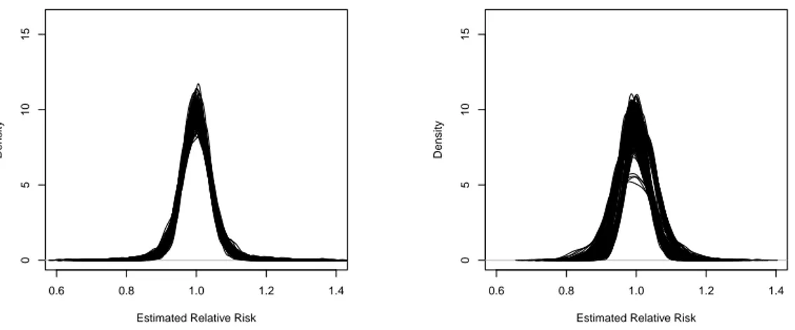
As we mentioned in the description of the model, we expect it to fit quite well the data when the relative risk is approximately constant over the region. To verify this, we simulated disease counts on the Auckland map keeping the risk population equal to that of the infant mortality example. We generated conditionally independent Poisson counts with the same relative rate, equals to 2 cases for every thousand inhabitants, in all areas. We fit the model proposed by Leroux, the BYM ICAR model and our own model to this data. In our model, we used only three matrices as in Section 2.1.
The posterior densities of the relative risk for the three models are presented in Figures 3.7 and 3.8 . In all models the estimates are centered in the correct value, equal to 1. However, our model with three components has the smallest variability. The density in this case is more concentrated around the true value. This means that, by including the matrix full of ones, we were able to smooth more the estimates. The other models did not consider the possibility of conditional correlation between all areas in the map and, therefore, in this kind of situation they have less precise estimates.
0.6 0.8 1.0 1.2 1.4
0
5
10
15
Estimated Relative Risk
Density
Figure 3.7: Posterior Densities of Relative Risk Bayesian estimates. Results using our model
3.2
Conclusions
In our model, we considered a precision matrix equal to a weighted average of increasing neighborhood matrices. One possibility we have not explored in this paper is to define a continuous version of this model. Let λ(t) be a probability density function defined for
t∈[0,1]andR(t)be a continuously defined precision matrix. Assume thatR(t) as a function of tis an injective function. The precision matrix of the mixture model is given then by
Q= 1
σ2 ∫ 1
0
3. Application and conclusion 22
0.6 0.8 1.0 1.2 1.4
0
5
10
15
Estimated Relative Risk
Density
0.6 0.8 1.0 1.2 1.4
0
5
10
15
Estimated Relative Risk
Density
Figure 3.8: Posterior Densities of Relative Risk Bayesian estimates. Results using Leroux (left) model and the ICAR estimates (right).
This model would allow different degrees of neighborhood and could be more flexible to adapt to empirical data. Another possible extension is to treat space-time data with a precision matrix that is a mixture of simpler precision matrices.
The BYM model is very popular but one problem with it is to find the appropriate spatial smoothing degree to estimate the relative risks. In fact, other authors have noticed its tendency to oversmooth the estimates in some cases (Best et al., 2005). The model we treat in this paper allows for the multiple definition of a smoothing neighborhood. In our model, the λj parameters control automatically this smoothing. The model can be specially useful
in the situation where the underlying risk is practically constant.
Bibliography
[1] Assunção, R. M. and Potter, J. E. (2002). A Bayesian space varying parameter model applied to estimating fertility schedules.Statistics in Medicine 14, 2057-2075.
[2] Assunção, R. M. (2003). Space varying coefficient models for small area data. Environ-metrics 14, 453–473.
[3] Assunção, R. M. and Krainski, E. T. (2009). Neighborhood Dependence in Bayesian Spa-tial Models.Biometrical Journal 51,851–869.
[4] Banerjee, S., Carlin, B. P. and Gelfand, A. E. (2004).Hierarchical Modeling and Analysis for Spatial Data. Chapman & Hall/CRC Monographs on Statistics & Applied Probability.
[5] Bernardinelli, L. and Montomoli, C. (1992). Empirical bayes versus fully bayesian analysis of geographical variation in disease risk. Statistics in Medicine 11,983–1007.
[6] Besag, J., York, J. and Mollié, A. (1991). RBayesian image restoration, with two applica-tions in spatial statistics. Annals of the Institute of Statistical Mathematics 43,1–20. [7] Best, N., Richardson, S. and Thomson, A. (2005). A comparison of Bayesian spatial models
for disease mapping.Statistical Methods in Medical Research,14, 35–59.
[8] Brezger, A., Kneib, T., and Lang, S. (2003). BayesX-software for Bayesian infer-ence based on Markov chain Monte Carlo simulation techniques (http://www.stat.uni-muenchen.de/ lang/).
[9] Carlin, B. and Banerjee, S. (2003). Hierarchical multivariate CAR models for spatio-temporally correlated survival data. Bayesian Statistics 7 (eds. J. M. Bernardo, J. O. Berger, A. P. Dawid, A. F. M. Smith), Oxford University Press, Oxford, 45–63.
[10] Choo, L. and Walker, G. (2008). A new approach to investigating spatial variations of disease. Journal of the Royal Statistical Society. Series A171, 395–405.
[11] Clayton, D. and Kaldor, J. (1987). Empirical Bayes Estimates of Age-Standardized Rel-ative Risks for Use in Disease Mapping.Biometrics 43,671–681.
3. Application and conclusion 24
[13] Elliot, P. and Wartenberg, D. (2004). Spatial Epidemiology: Current Approaches and Future Challenges.Environmental Health Perspect 112, 998–1006.
[14] Fahrmeir, L. and Lang, S. (2001). Bayesian inference for generalized additive mixed models based on Markov random field priors.Journal of the Royal Statistical Society, Series C 50,201–220.
[15] Gelfand, A. E., Hyon-Jung, K., Sirmans, C.F. and Banerjee S. (2003). Spatial Modeling with Spatially Varying Coefficient Processes.Journal of the American Statistical Associa-tion 98,2057–2075.
[16] Gelfand, A. E. and Vounatsou, P. (2003). Proper multivariate conditional autoregressive models for spatial data analysis. Biostatistics 4,11–25.
[17] White G. and Ghosh S. K. (2009). A stochastic neighborhood conditional autoregressive model for spatial data.Computational Statistics and Data Analysis 53,3033–3046. [18] Held, L., Natario, I., Fenton, S., Rue, H. and Becker, N. (2005). Towards joint disease
mapping.Statistical Methods in Medical Research 14,61–82.
[19] Held, L., Graziano, G., Frank, C. and Rue, H. (2006) RJoint spatial analysis of gastroin-testinal infectious diseases.Statistical Methods in Medical Research 15,465–480.
[20] Iosifescu M.Iosifescu, Finite Markov Processes and Their Applications. John Wiley and Sons, Chichester 1980.
[21] Iosifescu M. (1980). Finite Markov Processes and Their Applications.. Chichester: John Wiley and Sons.
[22] Jin, X. and Carlin, B. P. (2005). Multivariate parametric spatiotemporal models for county level breast cancer survival data.Lifetime Data Analysis 11,5–27.
[23] Jin, X., Carlin, B.P. and Banerjee, S. (2005). Generalized hierarchical multivariate CAR models for areal data. Biometrics 61, 950–961.
[24] Knorr-Held, L. and Besag, J. (1998). Modelling risk from a disease in time and space.
Statistics in Medicine 17,2045–2060.
[25] Knorr-Held, L. and Best, N. (2001). A shared component model for detecting joint and selective clustering of two diseases. Journal of the Royal Statistical Society, Series A164,
73–85.
[26] Kulldorff, M. (1997). A spatial scan statistic. Communications in Statistics Theory and methods,26, , 1481–1496.
3. Application and conclusion 25
[28] Leroux, B. G., Lei, X. and Breslow, N. (1999). Estimation of disease rates in small areas: A new mixed model for spatial dependence. In Statistical Models in Epidemiology; the Environment and Clinical Trials 179–192.
[29] Lang, S. and Fahrmeir, L. (2001). Bayesian generalized additive mixed models. A sim-ulation study. Journal of the Royal Statistical Society. Series C (Applied Statistics) 50,
201–220.
[30] MacNab C. and Dean C. B. (2001). Autoregressive Spatial Smoothing and Temporal Spline Smoothing for Mapping Rates.Biometrics 57,187–200.
[31] MacNab C. and Dean C. B. (2000). Parametric bootstrap and penalized quasi-likelihood inference in conditional autoregressive models.Statistics in Medicine 19,2421–2435. [32] Marshall, R. J. (1991). Mapping Disease and Mortality Rates Using Empirical Bayes
Estimators.Journal of the Royal Statistical Society. Series C (Applied Statistics) 40,283– 294.
[33] Martínez-Beneito, M. A., López-Quilez A. and Botella-Rocamora P. (2008). An autore-gressive approach to spatio-temporal disease mapping. Statistics in Medicine 27, 2874– 2889.
[34] Silva, G. L., Dean, C. B., Niyonsenga, T. and Vanasse, A. (2008). Hierarchical Bayesian spatiotemporal analysis of revascularization odds using smoothing splines. Statistics in Medicine 27,2381–2401.
[35] Sun, D. C., Tsutakawa, R. K., Kim, H. and He, Z. Q. (2000). Spatio-temporal interaction with disease mapping. Statistics in Medicine 19,2015–2035.
[36] Spiegelhalter DJ, Thomas A, Best NG, Lunn D. WinBUGS User Manual (Version 1.4). Cambridge: Mrc Biostatistics Unit, www.mrc-bsu.cam.ac.uk/bugs/, 2003.
[37] Spiegelhalter, D. J., Thomas, A., Best, N.G. and Lunn, D. (2003). Regression models and life tables (with discussion).WinBUGS User Manual (Version 1.4). Cambridge: Mrc Biostatistics Unit, www.mrc-bsu.cam.ac.uk/bugs/.
[38] Stern, H.S. and Cressie, N. (2000). Posterior predictive model checks for disease mapping models.Statistics in Medicine 19,2377–2397.
[39] Wall, M. (2004). A close look at the spatial structure implied by the car and sar models.
Journal of Statistical Planning and Inference 121, 311–324.
Appendix A
Demonstration of result (2.4)
A well known linear algebra result (Iosifescu (1989), page 45) states that, if P is a square matrix and each of the terms of the power matrix Pk tends to zero as k increases, then the inverse (I−P)−1 exists and it is given by
(I−P)−1 =I+P+P2+P3+. . .
To use this result with the matrix [I−λ2TA]−1, we need to show that the terms λl2[(TA)l]ij
of the power matrix approximate zero when the power l increases. This will be done finding an upper bound. Consider initially l= 2. We see that
λ22[(TA)2]ij = λ22 N ∑
k=1
aikakj
(λ1+λ2ni+λ3N)(λ1+λ2nk+λ3N)
= λ22
N ∑
k=1
aikakj/(nink)
(λ1/ni+λ2+λ3N/ni)(λ1/nk+λ2+λ3N/nk)
< λ 2 2
(λ1/N+λ2+λ3)2 N ∑
k=1 N ∑
k=1 aik
ni akj
nk ,
since ni ≤ N. As diag(1/n)A is an stochastic matrix, it can be seen as a transition matrix
of a random walk on the map with equal probabilities of jumping from a given area to any of its first-order neighbors. In this way, the second term in the multiplication is the probability that a random walk leaves sitei and reaches sitej in two steps and will be denoted byp(2)ij .
For an arbitrary l≥2, we have
λl2[(TA)l]
ij < (
λ2 λ1/N +λ2+λ3
)l p(l)ij
wherep(l)ij denotes the probability that the random walk goes fromitojinlsteps. Therefore,
A. Demonstration of result (2.4) 27
p(l)ij ∈[0,1]and since λ2/(λ1/N +λ2+λ3)<1, we have that
0≤ lim
l→∞λ l 2
[
(TA)l]
ij <l→∞lim (
λ2 λ1/N +λ2+λ3
)l
p(l)ij = 0.
This shows that the terms of the matrixλl 2
[
(TA)l]
Appendix B
Another interpretation for the terms
(
S
i
+
S
+
j
)
We can write Si+S+j in a way that reflects the structure of a complete graph. To make
this interpretation easier, we leave out the weights that multiply the terms of the adjacency matrix. We consider only the terms aij, which are one if i and j are neighbors and zero
otherwise. Therefore we have an approximation for Si+ that is given by
Si+≈ N ∑
j=1 mij =
(∞ ∑
k=0 a(k)i1
)
+
( ∞ ∑
k=0 a(k)i2
)
+· · ·+
(∞ ∑
k=0 a(k)iN
)
So we see that
Si+S+j ≈ [(∞
∑
k=0 a(k)i1
)
+· · ·+
(∞ ∑
k=0 a(k)iN
)] [(∞ ∑
k=0 a(k)1j
)
+· · ·+
(∞ ∑
k=0 a(k)N j
)]
=
[( ∞ ∑
k=0 a(k)i1
) (∞ ∑
k=0 a(k)1j
)
+· · ·+
(∞ ∑
k=0 a(k)iN
) (∞ ∑
k=0 a(k)N j
)]
| {z }
A +∑ l̸=m [( ∞ ∑ k=0 a(k)il
) (∞ ∑
k=0 a(k)mj
)]
| {z }
B
Consider Afirst. In this sum, we have the term
a(0)i1 a(0)1i +· · ·+a(0)iNa(0)2N
Asa(0)ij a(0)1j = 1 for all j, their sum is equal to N. InA, we also have the terms
a(0)i1 a(1)1i +· · ·+a(0)iNa(1)2N a(1)i1 a(0)1i +· · ·+a(1)iNa(0)2N .
Both of them count the possible ways of going from i to j in one step. If we consider the terms whose exponents summing up to 2, we have
B. Another interpretation for the terms (Si+S+j) 29
a(0)i1 a(2)1i +· · ·+a(0)iNa(2)2N a(1)i1 a(1)1i +· · ·+a(1)iNa(1)2N a(2)i1 a(0)1i +· · ·+a(2)iNa(0)2N
Each of these three terms counts the number of paths that go from ito j in 2 steps. In general, what we see is that if we take the terms whose exponent summing up to k, we will have terms of the following type:
a(0)i1 a(k)1i +· · ·+a(0)iNa(k)2N a(1)i1 a(k−1)1i +· · ·+a(1)iNa(k−1)2N
...
a(k)i1 a(0)1i +· · ·+a(k)iNa(0)2N
This means that the paths that go from ito j ink steps are countedk+ 1times. Therefore the term A can be written as
N+
∞ ∑
n=1
(number of paths fromito j inn steps) (n+ 1).
Now we analyze the termB. We can see that
N ∑ l=1 ∑ m̸=l ( ∞ ∑ n=0 a(n)il
) (∞ ∑
n=0 a(n)mj
)
=
(∞ ∑
n=0 a(n)i1
) (∞ ∑
n=0 a(n)2j
)
+
( ∞ ∑
n=0 a(n)i1
) (∞ ∑
n=0 a(n)3j
)
+· · ·+
( ∞ ∑
n=0 a(n)i1
) (∞ ∑
n=0 a(n)N j
)
+
(∞ ∑
n=0 a(n)i2
) (∞ ∑
n=0 a(n)1j
)
+
( ∞ ∑
n=0 a(n)i2
) (∞ ∑
n=0 a(n)3j
)
+· · ·+
( ∞ ∑
n=0 a(n)i2
) (∞ ∑
n=0 a(n)N j
) ... + (∞ ∑ n=0 a(n)iN
) (∞ ∑
n=0 a(n)1j
)
+
( ∞ ∑
n=0 a(n)iN
) (∞ ∑
n=0 a(n)2j
)
+· · ·+
( ∞ ∑
n=0 a(n)iN
) (∞ ∑
n=0
a(n)(N−1)j )
To see what this sum is counting, consider first the terms for which l = 1 and m = 2. In the same way that we did for the term A, we will analyze first the multiplication whose exponents sum up to 1:
[
B. Another interpretation for the terms (Si+S+j) 30
This counts twice the paths that go fromitojin two steps and that have to pass through an edge connecting areas 1 and 2. If this edge indeed exists in the neighborhood graph, this is just one of its possible paths. However, if 1 and 2 are not first-order neighbors, this edge does not exist. In this case, it is as if we include this (1,2) edge in the neighborhood graph and count the additional paths that were not considered before.
Lets know consider the multiplications whose exponents summing up to 2:
[
a(0)i1 +a(2)2j ]+[a(1)i1 +a(1)2j ]+[a(2)i1 +a(0)2j]
We see that they represent three times the number of paths of three steps that go from i
to j and pass through an edge (1,2), either truly present or not.
In general, for the terms whose exponent sum up k, we will count ktimes the number of possible paths of ksteps fromito j and that have to pass through an edge (1,2).
We just considered here the pair of sites 1 and 2, but the sum is over all possible pairs of sites. Therefore, the term B can be written in this way
∑
k̸=l ∞ ∑
n=0
(k+ 1) (number of paths of n steps fromito j that pass through edge k−l) .