Multivariate Misgivings: Is D a Valid Measure of Group and Sex Differences?

www.epjournal.net – 2013. 11(5): 1067-1076

¯ ¯ ¯ ¯ ¯ ¯ ¯ ¯ ¯ ¯ ¯ ¯ ¯ ¯ ¯ ¯ ¯ ¯ ¯ ¯ ¯ ¯ ¯ ¯ ¯ ¯ ¯ ¯

Original Article

Multivariate Misgivings: Is D a Valid Measure of Group and Sex Differences?

Abstract: In the study of group and sex differences in multivariate domains such as personality and aggression, univariate effect sizes may underestimate the extent to which groups differ from one another. When multivariate effect sizes such as Mahalanobis D are employed, sex differences are often found to be considerably larger than commonly assumed. In this paper, I review and discuss recent criticism concerning the validity of D as an effect size in psychological research. I conclude that the main arguments against D are incorrect, logically inconsistent, or easily answered on methodological grounds. When correctly employed and interpreted, D provides a valid, convenient measure of group and sex differences in multivariate domains.

Keywords: effect size, group differences, Mahalanobis D, measurement, sex differences

¯ ¯ ¯ ¯ ¯ ¯ ¯ ¯ ¯ ¯ ¯ ¯ ¯ ¯ ¯ ¯ ¯ ¯ ¯ ¯ ¯ ¯ ¯ ¯ ¯ ¯ ¯ ¯ ¯ ¯ ¯ ¯ ¯ ¯ ¯ ¯ ¯ ¯ ¯ ¯ ¯ ¯ ¯ ¯ ¯ ¯ ¯ ¯ ¯ ¯ ¯ ¯ ¯ ¯ ¯ ¯ ¯ ¯ ¯ ¯ ¯ ¯ ¯ ¯ ¯ ¯ ¯ ¯ ¯ ¯ ¯ ¯ ¯

Introduction

In the study of sex differences, accurate quantification is one of the most crucial tasks faced by researchers. The extent to which males and females are similar or different in their personality, cognition, and behavior is a source of lively debate, both within evolutionary psychology (see Stewart-Williams and Thomas, 2013, and commentaries in the same issue) and in the behavioral sciences at large (see Hyde, 2005, 2013).

under normality assumptions, the overlap between two groups relative to their joint distribution is 67% both when d = .50 (univariate) and when D = .50 (multivariate).

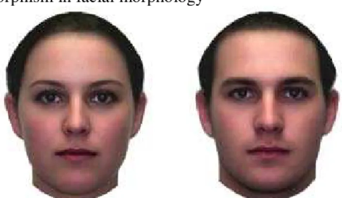
What is the rationale for employing a multivariate effect size? In a nutshell, small differences in multiple individual variables can add up to a much larger difference when all the variables—and their correlational structure—are considered simultaneously. A good example is provided by sexual dimorphism in facial morphology (see Figure 1). If one compares men and women on individual anatomical traits such as mouth width, forehead height, eyebrow thickness, and eye size, univariate differences tend to be relatively unimpressive. For example, a study by Ferrario, Sforza, Poggio, and Serrao (1996) found that men had higher foreheads (d = .40), longer jaws (d = .96), and wider faces than women (d = 1.08), whereas women had wider mouths (d = −.96). These are typical effect sizes in this domain. Their unsigned average is .85, corresponding to an overlap of 50% between the male and female distributions of facial traits. Given that male and female faces are discriminated with more than 95% accuracy by human observers (Bruce et al., 1993), this has to be a gross underestimate of the actual magnitude of sexual dimorphism. Indeed, when individual traits are integrated in a multivariate analysis, much larger differences are found. For example, Hennessy, McLearie, Kinsella, and Waddington (2005) applied D to sex differences in facial morphology and found an effect size of about D = 3.2, corresponding to an overlap of only 7% between the male and female distributions (Fig. 3 in Hennessy et al., 2005; note that D2 was plotted instead of D).

Figure 1. Sexual dimorphism in facial morphology

Note: Each average face is a composite of 24 pictures. Adapted with permission from Rhodes et al. (2004). Copyright 2004 by Elsevier Ltd.

methodological toolkit and revise existing ideas about the degree of psychological similarity between the sexes.

In this paper, I review and discuss the main critical arguments advanced by Hyde (2013) and Stewart-Williams and Thomas (2013). As I show below, some of these arguments are either incorrect or logically inconsistent, while the remaining ones can be easily answered on methodological grounds. When correctly employed and interpreted, D

stands as a valid, convenient measure of group and sex differences in multivariate domains.

Issues of Bias

Both Hyde (2013) and Stewart-Williams and Thomas (2013) argued that D is biased toward finding large group differences. The arguments they advanced can be interpreted in either a strong or a weak sense. When interpreted in a strong sense—that is, as intrinsic limitations of D—these arguments turn out to be fallacious or incorrect. Under a weaker interpretation, biases in the magnitude of D can be introduced by the accumulation of sampling error when many variables are included in the computation. In this sense, the critical arguments are correct, but they do not negate the validity of D and can be easily addressed on methodological grounds (see below).

In her review paper on gender similarities and differences, Hyde (2013) stated: . . . D is computed by taking the linear combination of the original variables (scores on emotional stability, dominance, vigilance, and so on) that maximizes the difference between groups. . . . this application of Mahalanobis D produces results that are biased toward finding a large difference because of taking a linear combination that maximizes group differences. (pp. 3.7-3.8)

In the strong sense, this argument is a fallacy. It is true that D is closely related to the linear discriminant function—a linear combination of variables that maximizes group differences on that function so as to achieve optimal discrimination between groups (McLachlan, 1992). However, it does not follow that the discriminant function is a biased

In a weaker sense, the argument may refer to the biases introduced by sampling error. Sample values of D tend to “capitalize on chance,” since stochastic deviations from zero in univariate effect sizes end up increasing the value of D in the sample by some amount. For this reason, sample estimates of D provide an upward-biased measure of group differences (discussed in Del Giudice, 2009). While this phenomenon is real, it is hardly unique to D. For example, sample estimates of explained variance (R2) in linear models (e.g., multiple regression) are biased upwards for much the same reason. A similar point was made by Stewart-Williams and Thomas (2013):

. . . it is a basic fact about the Mahalonobis D that the more unidimensional variables you include in your analysis, the larger the effect size will be. This has an awkward implication. No two groups will be identical on every measure. Even for very similar populations—New Zealanders and Australians, for example—there will inevitably be many variables for which there are small average differences. If you were to take enough of these variables and treat them as a single multidimensional variable, you could use Del Guidice’s [sic] method to “prove” that, psychologically, New Zealanders and Australians are virtually different species. . . . As long as you included enough unidimensional variables in the final multidimensional variable, the different-species conclusion would be inevitable. The inevitability suggests that it is the method that is driving the conclusion, rather than the true nature of the populations under discussion. (p. 168)

Interpreted in a strong sense, this argument is incorrect, as it moves from the false premise that adding more variables will inevitably increase D. In fact, D will not increase if the additional variables are linear combinations of other variables that are already in the computation. This includes—but is not limited to—the special case in which two or more variables are perfectly correlated with one another. In substantive terms, adding variables in the ideal case will increase D only insofar as they provide unique additional information

about group differences. As one gathers more and more real-world variables in the same domain, the likelihood that new variables will be statistically redundant with those already included in the model increases, and the marginal increase in D diminishes accordingly.

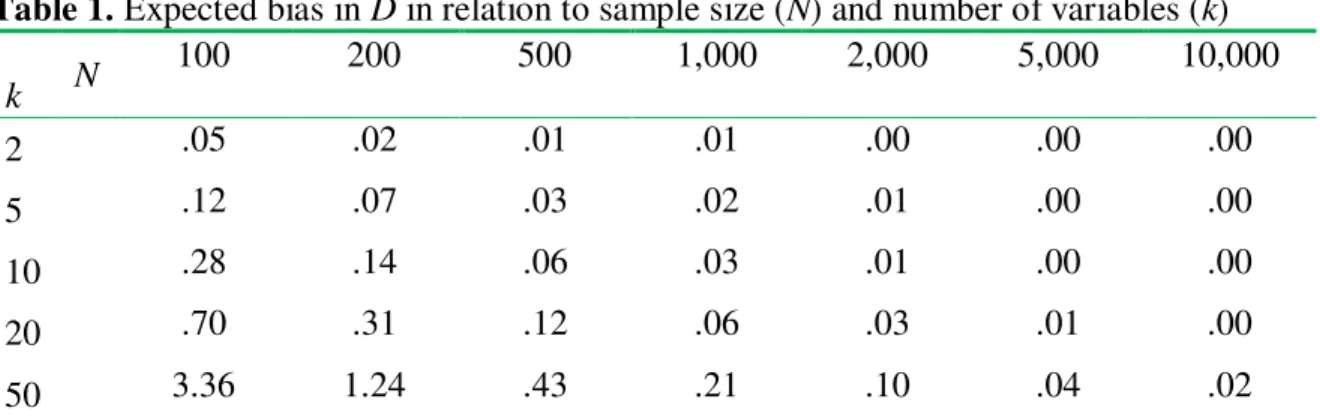
Table 1. Expected bias in D in relation to sample size (N) and number of variables (k)

k N

100 200 500 1,000 2,000 5,000 10,000

2 .05 .02 .01 .01 .00 .00 .00

5 .12 .07 .03 .02 .01 .00 .00

10 .28 .14 .06 .03 .01 .00 .00

20 .70 .31 .12 .06 .03 .01 .00

50 3.36 1.24 .43 .21 .10 .04 .02

Notes: Univariate effect sizes in the population are normally distributed with mean 0 and standard deviation 1. Simulations are based on 1,000 replications for each combination of parameters, assuming groups of equal size (N/2). Values are rounded to two digits.

Based on simulation results, the following rule of thumb can be suggested. In most research contexts, a bias of less than .05 can be regarded as very small; indeed, many investigators treat d = .10 as a “trivial” effect size. To keep the expected bias below the .05 threshold, one should have at least 100 cases for each variable included in the computation (see Table 1). Equivalently, the number of variables should be k≤ N/100. The rule holds in a broad range of realistic conditions (i.e., for values of the standard deviation of univariate effect sizes ranging from .30 to 3.00).

In light of these results, it is useful to consider the likely magnitude of bias in the study of sex differences in personality by Del Giudice and colleagues (2012), the main target of criticism from Hyde (2013) and Stewart-Williams and Thomas (2013). In that study, 15 personality variables were considered with a sample size of N = 10,261. This sample size is more than adequate for minimizing bias; indeed, simulations show an expected bias close to zero, while the measured effect size was D = 2.71. Also, the confidence interval on D was very narrow, from 2.66 to 2.76 (see Del Giudice et al., 2012). Clearly, the large sex differences in personality found in the study cannot be explained away as biases due to sampling error.

While sampling error tends to inflate D, it should be kept in mind that measurement

error has the opposite effect, and tends to produce downward-biased values of D (as well as

d; see Del Giudice et al., 2012). Thus, accurate estimates of D require two independent conditions: (a) the ratio of cases to variables should be sufficiently large, and (b) measurement error in the original variables should be minimized. The latter can be obtained by employing latent variable modeling as in Del Giudice et al. (2012), or approximated by disattenuating correlations and univariate effect sizes (Del Giudice, 2009; Del Giudice et al., 2012).

measurement reliability (Del Giudice, 2009). In addition, confidence intervals on D— which take into account both k and N—should be computed whenever possible to check the reliability of sample estimates (see Reiser, 2001; Zou, 2007). Note that minimizing bias (i.e., achieving accuracy) does not guarantee a narrow confidence interval (i.e., achieving

precision); much larger samples are usually required to obtain a precise estimate of D. Finally, it should be stressed that D—like any other statistical tool—can only yield meaningful results when it is employed in a reasonable, theoretically justified way. In particular, D is especially useful when the variables included in the computation are part of a well-defined construct such as the 16PF model of personality (Del Giudice et al., 2012), the three-factor model of aggression (Del Giudice, 2009), or the anxiety/avoidance model of romantic attachment (Del Giudice, 2011). Adding dozens of conceptually unrelated variables to the mix in order to increase D—as implied by Stewart-Williams and Thomas in the passage above—would not make sense in most situations, just as it would not make sense to add dozens of unrelated predictors to a multiple regression model simply to obtain larger and larger values of R2 (see Burnham and Anderson, 2002; Cohen, Cohen, West, and Aiken, 2003).

Issues of Interpretation

In addition to their methodological criticism, Hyde (2013) and Stewart-Williams and Thomas (2013) raised the issue of how D can be interpreted in substantive terms. Both argued that D poses serious problems of interpretation—a severe stumbling block if D is to be employed to address important scientific questions about group and sex differences.

In her commentary on Del Giudice and colleagues (2012), Hyde (2012) argued that

D provides literally uninterpretable results. The claim was repeated in the following passage from Hyde (2013):

. . . this difference or distance is along a dimension in multivariate space that is a linear combination of the original variables, but this dimension is uninterpretable. What does it mean to say that there are large [sex] differences in personality, lumping together distinct aspects such as emotional stability, dominance, and vigilance? Certainly contemporary personality theorists do not argue that there is a single dimension to personality. (pp. 3.7-3.8)

While superficially appealing, Hyde’s criticism is actually off target. To begin with, measuring differences between groups in a multivariate space does not imply that those differences can or should be reduced to “a single dimension.” In fact, the opposite is true: If variation in personality really were one-dimensional, it would make no sense to compute a multivariate effect size to begin with. The weakness of this criticism becomes fully apparent if one replaces “personality” with “facial morphology” in the quotation above:

“What does it mean to say that there are large [sex] differences in facial morphology, lumping together distinct aspects such as eyebrow thickness,

The argument is thus revealed as a non sequitur: clearly, it makes perfect sense to speak of large sex differences in facial morphology—“lumping together” differences in multiple traits such as face width and eye size—with no need to assume that individual differences in facial traits can be reduced to a single dimension (see Figure 1). Far from being uninterpretable, the resulting axis of individual variation can be easily defined as

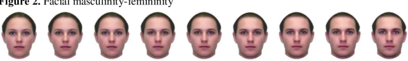
facial masculinity-femininity (e.g., Hennessy et al., 2005) or some equivalent term. As is apparent from Figure 2, facial masculinity-femininity is a very recognizable configural trait that summarizes a multitude of individual morphological differences, even if it does not correspond to any specific anatomical structure. In exactly the same way, multivariate sex differences in personality can be interpreted as defining an axis of individual variation in

personality masculinity-femininity (see Lippa, 2001). Whatever the exact terms chosen to denote these constructs, there is nothing mysterious about their interpretation. Of course, the global differences measured by D are not intended to replace univariate effects but rather supplement them, as stressed in Del Giudice (2009).

Figure 2. Facial masculinity-femininity

Notes: The figure shows a sequence of morphed faces, from 100% female to 100% male. Adapted with permission from Rhodes et al. (2004). Copyright 2004 by Elsevier Ltd.

Stewart-Williams and Thomas (2013) raised a related but distinct point:

. . . the most damning criticism of the method, in our view, is that adding new unidimensional variables increases the overall effect size regardless of the direction of the effect for each variable. Aggression provides a good example. If we look at physical aggression and verbal aggression in isolation, the average score for each is higher for men than for women. . . . If we combine these variables and treat them as a single multidimensional variable, the effect size of the sex difference is noticeably larger than for either alone. If we then add

indirect aggression, the effect size is larger again (Del Guidice [sic], 2009). The natural interpretation is that men are much more aggressive than women, and that the difference is much larger than we would think if we looked at each unidimensional variable on its own, or if we only considered physical and verbal aggression. The problem is, however, that for indirect aggression, the sex difference actually goes in the other direction: The average score for women is slightly higher than that for men. . . . This raises serious questions about how to interpret any results gleaned from this method. (p. 168)

considered. The correct interpretation is that males and females differ in their patterns of aggression (see Del Giudice, 2009), and that the average distance between the sexes along the abstract axis of masculinity-femininity in aggression patterns is slightly less than one standard deviation (estimated D = .89 to 1.01 in Del Giudice, 2009). The fact that Stewart-Williams and Thomas regard their incorrect interpretation as “natural” seems to reflect a lack of appreciation of how multivariate differences work. The same difficulty surfaces when these authors misquote Del Giudice and colleagues (2012) in the following passage:

Del Guidice [sic] and colleagues . . . found an effect size of 2.71 for the sex difference in “global personality.” (p. 168)

In fact, the term “global personality” is nowhere to be found in our paper; the topic of our investigation was the radically different concept of global sex differences in personality (contrasted with univariate sex differences in individual personality traits). Far from reducing all personality to a single global dimension, D isolates the axis of variation that best discriminates between males and females, and permits quantification of average sex differences in personality masculinity-femininity; even more usefully, it can be translated into a summary measure of the overall statistical overlap between the male and female distributions.

In summary, Hyde’s argument turns out to be a non sequitur, while the criticism raised by Stewart-Williams and Thomas seems to reflect an incorrect reading of Del Giudice (2009) rather than an intrinsic limitation of D. In both cases, the authors seem to be forcing multivariate effects into the more familiar univariate framework, with predictably misleading results. When D is properly framed as a multivariate distance, it poses no special problems of interpretation. Again, univariate and multivariate effect sizes are not mutually exclusive—they should always be considered together, to gain as much insight as possible into the nature of the investigated construct.

Conclusion

Psychologists routinely measure and discuss sex differences as collections of univariate effects, even when dealing with highly multidimensional domains such as personality, emotional experience and expression, cognitive abilities, vocational interests, and sexuality (e.g., Hyde, 2013). This would be akin to measuring sexual dimorphism in face or body shape by considering only one trait at a time, without ever trying to aggregate variables into the bigger picture of global similarity/dissimilarity patterns. Predictably, this approach can easily lead researchers to underestimate the magnitude of sex differences in many important domains.

must be commensurate with the number of variables included in the computation in order to minimize bias; having at least 100 cases per variable should prove a reasonable rule of thumb in most research contexts. Other methodological issues are discussed in Del Giudice (2009). By adding D to their analytical toolkit, researchers who deal with group and sex differences will increase their ability to see the forest for the trees, and gain a deeper appreciation of the many ways in which human beings resemble and differ from one another.

Acknowledgements: I am indebted to Drew Bailey for his insightful comments and suggestions.

Received 14 October 2013; Accepted 29 November 2013

References

Bruce, V. A., Burton, M., Hanna, E., Healey, P., Mason, O., Coombes, A., . . . Linney, A. (1993). Sex discrimination: How well do we tell the difference between male and female faces? Perception, 22, 131-152.

Burnham, K. P., and Anderson, D. R. (2002). Model selection and multimodel inference: A practical information–theoretic approach (2nd ed.). New York: Springer.

Cohen, J., Cohen, P., West, S. G., and Aiken, L. S. (2003). Applied multiple regression/correlation analysis for the behavioral sciences (3rd ed.). Hillsdale, NJ: Erlbaum.

Del Giudice, M. (2009). On the real magnitude of psychological sex differences.

Evolutionary Psychology, 7, 264-279.

Del Giudice, M. (2011). Sex differences in romantic attachment: A meta-analysis.

Personality and Social Psychology Bulletin, 37, 193-214.

Del Giudice, M., Booth, T., and Irwing, P. (2012). The distance between Mars and Venus: Measuring global sex differences in personality. PLoS ONE, 7, e29265.

Ferrario, V. F., Sforza, C., Poggio, C. E., and Serrao, G. (1996). Facial three-dimensional morphometry. American Journal of Orthodontics and Dentofacial Orthopedics, 109, 86-93.

Hennessy, R. J., McLearie, S., Kinsella, A., and Waddington, J. L. (2005). Facial surface analysis by 3D laser scanning and geometric morphometrics in relation to sexual dimorphism in cerebral–craniofacial morphogenesis and cognitive function. Journal of Anatomy, 207,283-295.

Huberty, C. J. (2005). Mahalanobis distance. In B. S. Everitt and D. C. Howell (Eds.),

Encyclopedia of statistics in behavioral science. Chichester: Wiley.

Hyde, J. S. (2005). The gender similarities hypothesis. American Psychologist, 60, 581-592.

Hyde, J. S. (2012). The distance between North Dakota and South Dakota. Retrieved on

Oct 10, 2013 at

Hyde, J. S. (2013). Gender similarities and differences. Annual Review of Psychology.

Advance online publication.doi: 10.1146/annurev-psych-010213-115057.

McLachlan, G. J. (1992). Discriminant analysis and statistical pattern recognition. Hoboken, NJ: Wiley.

R Core Team (2012). R: A language and environment for statistical computing. R Foundation for Statistical Computing, Vienna, Austria. URL:

Reiser, B. (2001). Confidence intervals for the Mahalanobis distance. Communications in Statistics: Simulation and Computation, 30, 37-45.

Rhodes, G., Jeffery, L., Watson, T. L., Jaquet, E., Winkler, C., and Clifford, C. W. G. (2004). Orientation-contingent face aftereffects and implications for face-coding mechanisms. Current Biology, 14, 2119-2123.

Salkind, N. J. (Ed.) (2007). Encyclopedia of measurement and statistics. Thousand Oaks, CA: Sage.

Stewart-Williams, S., and Thomas, A. G. (2013). The ape that thought it was a peacock: Does evolutionary psychology exaggerate human sex differences? Psychological Inquiry, 24,137-168.

Zou, G. Y. (2007). Exact confidence interval for Cohen’s effect size is readily available.