Adaptive filtering using Higher Order Statistics (HOS)
Abdelghani Manseur1, Daoud Berkani2 and Abdenour Mekhmoukh3
1
Department of Electrical Engineering, Kasdi Merbah University Ouargla, Algeria
2
Department of Electronics, Polytechnical National School Algiers, Algeria
3
Department of Electrical Engineering, Abderahmane Mira University Bejaia, Algeria
Abstract
The performed job, in this study, consists in studying adaptive filters and higher order statistics (HOS) to ameliorate their performances, by extension of linear case to non linear filters via Volterra series.
This study is, principally, axed on:
Choice of the adaptation step and convergence conditions.
Convergence rate.
Adaptive variation of the convergence factor, according to the input signal.
The obtained results, with real signals, have shown computationally efficient and numerically stable algorithms for adaptive nonlinear filtering while keeping relatively simple computational complexity.
Keywords:Convergence factor, Adaptive filtering, Equalization, Higher Order Statistics (HOS), non linear filters, Volterra series.
1. Introduction
Filtering is known as adaptive, if there is modification of its parameters with each time there is a change in the input signal.
The algorithm of adaptive filtering updates, recursively, the coefficients of the filter, in order to enable him to follow the evolution of the process. If it is stationary, the algorithm must converge towards the optimal solution of Wiener, if not it will have a capacity to follow the variations of the statistical sizes of the process.
In spite of the great importance of the filters and linear systems of modeling in large ranges of situations, there exist many applications in which they post their limits of performance. In the presence of multiplicative noise, for example, the performances of the linear filters are insufficient. For this reason, recently, much of attention was given to nonlinear modeling systems via Volterra series [1]. In the family of the nonlinear filters we find the
class of the polynomial filters (of Volterra). This type of filter finds its applications in many fields like signal processing, the communication systems, the echo cancellation and the systems identification [2].
In this work, we will extend the study of linear adaptive filtering to the nonlinear systems using the Volterra series in the adaptive equalization of the nonlinear channels of communication, for the acoustic echo cancellation.
The key point of the Volterra filters is that, the output of the filter is linearly dependant compared to the filter coefficients [1], [3] and [4].
2. Optimal filter of Wiener
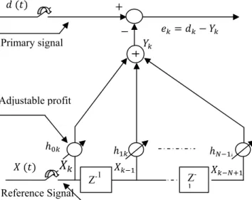
Let us consider the following figure 1, where is represented a transverse adaptive filter Hk [5].
The goal of the optimal filter is to obtain at output an answer nearest possible to the desired signal when the input is a sequence .
Several cost functions makes it possible to obtain an optimal configuration of the filter. Among them, the Mean Square Error (MSE) is most usual, because it leads to complete and simple mathematical developments; moreover, it provides a single solution.
The optimal filter of Wiener minimizes the Mean Square Error noted , which is given by:
| |
The error signal will be given as follows:
From where:
After development we will have:
Where:
| | Is the variance of the desired signal.
Is the vector of intercorrelation between the input signal and the desired signal .
Is the matrix of autocorrelation of the input signal . This matrix is definite positive, of Toeplitz.
The optimum vector of the coefficients ∗ of the filter is obtained by the cancellation of the gradient of the criterion:
J ∂H∂J E e ∂H ∂e
Let us pose J , we will have:
∗
That we can simplify in the form:
∗
Thus:
∗
More known as Wiener-Hopf equation [6], [7] and [8]. By combining the equations (4) and (8), we can lead to the algorithm of the gradient given as follows:
Where represents the factor of convergence or adaptation step, which is a positive constant, that controls the rate of convergence of the algorithm.
3. Choise of the algorithm
The adaptive filters can be classified according to the choices which are made on the following criteria [9], [10]:
Speed of convergence.
Capacity to follow the non linearities of the system.
The stability and precision of the estimate of the parameters of the filter.
The Minimal Mean Square Error.(MMSE)
The order of the filter.
4. Applications of the adaptive filtering
Adaptive filtering finds its applications in various fields [6], [9] and [10]
Identification of systems.
The prediction.
Opposite modeling.
The interferences cancellation.
5. The variable step adaptation LMS
In the Least Mean Square (LMS) algorithm, the step adaptation is fixed (time invariant). Some is the coefficients of the initial vector, the algorithm converges and becomes stable if the factor of convergence, or the step adaptation, μ satisfied the relation [8].
Where is the maximum eigen value of the autocorrelation matrix .
Update of the step adaptation
In order to increase the performances of the algorithm, in particular in a non stationary case, a recursive adaptation of the convergence factor becomes necessary, but while keeping a reasonable complexity of calculation.
With an aim of reducing mathematical complexity, Kamal Meghriche [5] proposes a new iterative law of update of the step of convergence in two stages.
Adjustable profit Primary signal
Reference Signal
Fig. 1 Transverse adaptive linear filter
Z-1 Z
∑
Where N represents the order of the filter, and initial convergence factor.
After the first N iterations of initialization, the recursive form of the convergence step becomes:
∆ ∆
Where:
∆
To simplify the expression (12), we pose
′
What will lead us to the following relation:
′ ′
After the N first iterations , ′ is given by:
′ ′
Therefore, the convergence of the algorithm is satisfied if:
′
Moreover , which is the adjustment error, becomes:
≅ ′
The general expression of the algorithm becomes:
′
6. Modeling of the non linear systems via the
Volterra series
In this work, we will try to extend the study of the linear systems to the nonlinear systems via the Volterra series. Let us recall that a linear system is defined by the convolution of an input signal by a filter.
The model illustrated by (20) cannot give a satisfactory representation of all the systems, for that, an extension to the nonlinear systems via the Volterra series proves to be necessary.
The input/output relation of a Volterra filter, which can be described in the form of a multidimensional convolution [1] and [11], is given by [12], [13] and [14]:
∞
∞ ∞
∞ ∞
∞
,
, ,
∞
∞ ∞
∞ ∞
∞
⋯
Where , , , , , , .. are the cores of Volterra [1], [2] and [14].
In the equation (21), , , , . . . is the th order of the discrete core of Volterra [14].
Another representation can be found in the literature [1], [3], [11] and [15]. But in our study, we always base our self on the first model.
∞
∞ ∞
∞ ∞
∞
,
, ,
∞
∞ ∞
∞ ∞
∞
⋯
Where is the shift term (offset term) [1].
One of the problems of the polynomial filters is that they require a great number of coefficients to characterize a nonlinear process. This problem can be solved by the use of a recursive polynomial structure which, as in the linear case, requires a reduced number [3]. Therefore, in the majority of the cases, we limit our self to the first two terms and , .
In the case of a nonlinear Volterra filter, we would like to find the coefficients of the filter which minimize the Mean Square Error (MSE) given by the equation (23), when the output of the filter of Wiener is given by the equation (24).
∞
∞ ∞
∞ ∞
∞
,
Where is the Minimal Mean Square Error (MMSE) leading to the Wiener optimal solution.
For that, we form the data vector and the coefficients vector , in continuation we will be able to obtain a compact vectorial representation (24).
Thus we will have [12]:
… . . a
… . . b
. . .
… . c
, , … , … ,
. d
Where N: Is the linear core order of the filter . M: Is the quadratic core order of the filter .
While using (25), we will be able to give the two vectors and :
. a
. b
The dimensions of the vectors , is ,
and those of , is / . Then, the
dimensions of and become [12]. That is due to the fact that the quadratic core , is symmetrical [4].
Therefore, the vectorial form of the output of the filter will be given by:
According to equations, (23) and (27), we can deduce, that [5]:
We proceed in the same way as in the linear case of the Wiener filter, the coefficients of the optimal filter are obtained by cancelling the gradient from in ratio with the filter coefficients, which leads us, [5], with:
With . a And . b
If we divided the data vector in two parts, [12], we will have, [5]:
Where and represent, respectively, the linear and quadratic part of the filter.
In this case, contains the statistics of order two, three and four [5].
Thus
Then
From (33), we can deduce that [5]:
Is a matrix from by container
the statistics of order two.
Is a matrix from by /
container the statistics of order three.
Is a matrix from / by
/ container the statistics of order four.
For recall, one of the most important properties of the Volterra filters is that the output of the filter is linearly dependant compared to the parameters on the cores [1], [3] and [4]. Moreover, they can be interpreted as being multidimensional convolutions [1] and [11].
7. Volterra adaptive filtering with variable
step adaptation
With an aim of improving the performances of the Volterra adaptive filter, we base our self on the diagram of figure 3.
According to figure 3, the update of the adaptive filter coefficients is given by:
The starting point for the determination of the adaptation steps of the two parts linear and quadratic, which ensure the convergence of the algorithm, is given by [5]:
∑ , ,
Where Is the linear core order . Is the quadratic core order.
After and first iterations of initialization, the steps of adaptation and can be given, by carrying out the change of variable, by:
′ ′ ∆ ,
Where:
∆
∆
What leads us to the following reformulation:
′
′
Since ′ is the filter linear part adaptation step, therefore, the determination of the conditions of convergence is the same one as that of the LMS with a fixed adaptation step [5]:
For the determination of the nonlinear part convergence conditions, we proceed as follows:
From the equation (37), it results:
′
′
Binary Signal Pseudo Random
Gaussian Additive White Noise
Fig. 3 Equalization of a numerical channel using Higher
Order Statistics (HOS). (GAWN)
What can lead to the following equation:
Where is the transposed operator.
′
′
While posing and , (40)
becomes:
According to the same reasoning, we can obtain (43):
Since the input signal, Binary Signal Pseudo Random (BSPR), is limited, and by applying the Milosavljević condition of convergence [16]:
By making the change of variable according to: and
We will have:
While writing:
Г Г Г
Where:
Г
Г
Then, to have the convergence of the algorithm, it is
enough to pose Г Г , which carries out us to
′ ′
Thus:
Finally, to have the algorithm convergence, it is enough to have the initial value of the adaptation step of the nonlinear part lower than that of the linear part.
8. Acoustic echo cancellation
Acoustic echo is a problem encountered in telecommunication, in particular in the applications of teleconference. The echo comes from the passage of the signal sent through a channel, for example a room, in the case of telephony free hands. Therefore, the echo is the phenomenon in which a delayed and distorted version of a sound is reflected and returned towards the source [17]. It is thus, desirable to be able to eliminate this echo at the reception from the signal. This is made possible using adaptive filtering.
Principle of the acoustic echo cancellation
The diagram Fig. 4, [17], represents a traditional system of echo cancellation in a communication system (telephone free hands, teleconference, …).
Let us consider, therefore, two interlocutors A and B, the first being to imagine on the right of the Figure, in front of the microphone, and the second on the left side, at the other end of the transmission channel and in a symmetrical environment with that of A. If we places as regards interlocutor A, this last is at the origin of an audio signal
who additively mixes by the microphone to an audio disturbing signal , coming from the high speaker of the telephone, and of which the origin is essentially to find in acoustic information collected by the microphone in front of which speaks the speaker B. This disturbing signal is called echo because if it is turned over via the communication channel, the speaker B will get along indeed in echo.
Obtained results
The aim of this part is to put forward the performances of our filter in the acoustic echo cancellation. For that, the diagram of figure 5 is retained [17].
In figure 5, we finds the speech useful signal , as well as the echo signal , which is the filtered version of the speech signal of the remote speaker by the unknown way, which is added to form signal y . Signal forms, also, the excitation of the main road. Therefore, to eliminate the noise , the nonlinear Volterra filter, must identify the unknown way as well as possible to find at exit of our system a speech signal nearest possible to the useful signal .
Fig. 6 represents desired signal and Output signal of the adaptive filter It is noticed that the evolution of the output signal of the filter follows perfectly that of the desired signal.
Fig. 7 represents the comparaison between desired signal and output signal of the adaptive filter. It is noticed that the evolution of the output signal of the filter follows perfectly that of the desired signal, even if there is a light going beyond.
Fig. 5 modeling of the adaptive echo cancellation Unknown
system
Nonlinear adaptive filter
-0 2000 4000 6000
-0.8 -0.6 -0.4 -0.2 0 0.2 0.4 0.6
Desired signal
Iterations number
A
m
pl
it
ude
0 2000 4000 6000
-0.6 -0.5 -0.4 -0.3 -0.2 -0.1 0 0.1 0.2 0.3 0.4
Output signal of the adaptive filter
Iterations number
A
m
pl
it
ude
Fig. 6 Desired signal and Output signal of the adaptive filter
0 1000 2000 3000 4000 5000 6000
-0.8 -0.6 -0.4 -0.2 0 0.2 0.4 0.6
Desired signal and output signal of the adaptive filter
Iteration number
A
m
p
lit
u
d
e
Output signal of the adaptive filter Desired signal
9. Conclusions
In this work, we saw an outline on adaptive filtering and the various selection criteria of the algorithm like its cases of applications. Then, a study of the Least Mean Squares (LMS) algorithm was made, while giving a version of variable step adaptation.
An extension of the linear case to nonlinear case of the adaptive filters is possible, by using Higher Order Statistics (HOS) and the Volterra series, by keeping, relatively, a mathematical simplicity of calculation.
An application of the nonlinear Volterra filter with variable step adaptation, with real speech signal, for cancellation of acoustic echo, showed the capacity of this last to identify the various sources of disturbance.
References
[1] G. L. Sicuranza, “Quadratic filters for signal processing,” Proc. IEEE,
vol. 80, no. 8, pp. 1263–1285, 1992.
[2] G. L. Sicuranza, A. Bucconi, P. Mitri, “Adaptive Echo Concellation
with Nonlinear Digital Filters”, Proceedings of ICASSP 84, pp. 3.10.1-4,
March 1984.
[3] Enzo Mumolo, Alberto Carini, Recursive Volterra Filters with
Stability Monitoring, Dipartimento di Electrotecnica, Electronica ed
Informatica, Universita di Trieste, Via Valerio 10, 34127 Trieste, Italy.
[4] Robert D. Nowak, Member , IEEE, Penalized Least Squares
Estimation of Volterra Filters and Higher Order Statistics, Department of
Electrical Engineering, Michigan State University, 206 Engineering
Building, East Lansing, MI 48824-1226.
[5] Kamal Meghriche, Filtrage adaptatif utilisant les statistiques d’ordre
supérieur, thèse de doctorat d’état en électronique, Ecole Nationale
Polytechnique d’Alger, Mai 2007.
[6] Freddy Mudry, Signaux et Systèmes, 6éme partie, Filtrage adaptatif
Codage de la parole, Ecole d’ingénieurs du Canton de Vaud, 2005.
[7] C.L. Nikias and M.R. Raghuveer, “Bispectrum estimation: A digital
signal processing framework,” Proceedings of the IEEE, vol. 75, no. 7,
pp. 869–891, July 1987.
[8] B. Widrow, J.R. Glover, J. McCool, J. Kaunitz, C. Williams, R.
Hearn, J. Zeidler, E. Dong, and R. Goodlin, “Adaptive noise cancelling:
Principles and applications,” Proc. of the IEEE, vol. 63, no. 12, pp. 1692–
1716, December 1975.
[9] J.F. Bercher, et P. Jardin, Introduction au filtrage adaptatif, ESIEE
Paris.
[10] Jacob Benesty, Traitement des signaux numériques-II, Filtrage
adaptatif et analyse spectral, Note de cours, INRS-EMT.
[11] D. W. Griffith, J. R. Arce, “Partially decoupled Volterra filters:
formulation and LMS adaptation,” IEEE Transactions on Signal
Processing, vol. 45, no. 6, pp. 1485–1494, 1997.
[12] F. Kuerch, and W. Kellermann, Proportionate NLMS Algorithm for
Second-order Volterra Filters and it’s Application to Nonlinear Echo
Cancellation, Telecommunications Laboratory, University of
Eriangen-Nuremberg, Cauerstr. 7 D-91058 Eriangen, Germany.
[13] Eduardo L. O. Batista, Orlando J. Tobias, and Rui Seara, Fully and
Partially Interpolated Adaptive Volterra Filters, LINSE-Circuits and
Signal Proccessing Laboratory, Departement of Electrical Engineering,
Federal University of Santa Catarina, 88040-900 – Sc – Brazil.
[14] A. Asfour, K. Raoof, and J. M. Fournier, Nonlinear Identification of
NMR Spin Sysrems by Adaptive Filtering, Journal of Magnetic
Resonance 145, 37-51 (2000).
[15] Abhijit A. Shah, Advisor: Dr. Tufts, Development and Analysis of
Techniques for Order Determination and Signal Enhancement, PhD
dissertation, University of Rhod Islands, 1994.
[16] C. Milosavljevic, “General conditions for the existence of a
quasisliding mode on the switching hyperplane in discrete variable
structure systems,” Automation & Remote Control, no. 46, pp. 307–314,
1985.
[17] Farid Ykhlef, Réduction de bruit et contrôle d’écho pour les
applications radio mobile et audioconférence, thèse de doctorat d’état en
électronique, laboratoire signal et communications, Ecole Nationale