Friction and mixing effects on potential vorticity for bottom current crossing a marine strait: an application to the Sicily Channel (central Mediterranean Sea)

(1)

OSD

11, 2495–2532, 2014

Friction and mixing effects on potential vorticity for bottom current crossing

a marine strait

F. Falcini and E. Salusti

Title Page

Abstract Introduction

Conclusions References

Tables Figures

◭ ◮

Back Close

Full Screen / Esc

Printer-friendly Version Interactive Discussion

Discussion

P

a

per

|

Discus

sion

P

a

per

|

Discussion

P

a

per

|

Discussion

P

a

per

|

Ocean Sci. Discuss., 11, 2495–2532, 2014 www.ocean-sci-discuss.net/11/2495/2014/ doi:10.5194/osd-11-2495-2014

This discussion paper is/has been under review for the journal Ocean Science (OS). Please refer to the corresponding final paper in OS if available.

Friction and mixing e

_ff

ects on potential

vorticity for bottom current crossing

a marine strait: an application to the Sicily

Channel (central Mediterranean Sea)

F. Falcini and E. Salusti

CNR-ISAC, Via del Fosso del Cavaliere 100, 00133 Rome, Italy

Received: 8 August 2014 – Accepted: 1 October 2014 – Published: 18 November 2014

Correspondence to: F. Falcini ([email protected])

(2)

OSD

11, 2495–2532, 2014

a marine strait

Title Page

Tables Figures

◭ ◮

Back Close

Full Screen / Esc

Discussion

P

a

per

|

Discus

sion

P

a

per

|

Discussion

P

a

per

|

Discussion

P

a

per

Abstract

We discuss here the evolution of vorticity and potential vorticity (PV) for a bottom

cur-rent crossing a marine channel in shallow-water approximation, focusing on the effect

of friction and mixing. We argue that bottom current vorticity is prone to significant sign

changes and oscillations due to topographic effects when, in particular, the current

5

flows over the sill of a channel. These vorticity variations are, however, modulated by frictional effects due to seafloor roughness and morphology. Such behavior is also re-flected in the PV spatial evolution, which shows an abrupt peak around the sill region. Our theoretical findings are discussed by means of in situ hydrographic data related to the Eastern Mediterranean Deep Water, i.e., a dense, bottom water vein that flows

10

northwestward, along the Sicily Channel (Mediterranean Sea). Indeed, the narrow sill of this channel implies that friction and entrainment need to be considered. Small tidal effects in the Sicily Channel allow for a steady theoretical approach. Our diagnoses on vorticity and PV allow us to obtain general insights about the effect of mixing and fric-tion on the pathway and internal structure of bottom-trapped currents flowing through

15

channels and straits, and to discuss spatial variability of the frictional coefficient. Our

approach significantly differs from other PV-constant approaches previously used in

studying the dynamics of bottom currents flowing through rotating channels.

1 Introduction

An ongoing debate in diagnostic model for currents that flow over a sill in a

rotat-20

ing channel with varying cross sections concerns the effect of friction and mixing,

which clearly play an important role in the presence of morphological constraints (Pratt et al., 2008; Pratt and Whitehead, 2008). Idealized models for marine currents flow-ing through rotatflow-ing channels (e.g., Whitehead et al., 1974; Gill, 1977; Borenas and Lundberg, 1986, 1988; Killworth, 1992) have provided basic ideas about their

hy-25

(3)

OSD

11, 2495–2532, 2014

a marine strait

Title Page

Tables Figures

◭ ◮

Back Close

Full Screen / Esc

Discussion

P

a

per

|

Discus

sion

P

a

per

|

Discussion

P

a

per

|

Discussion

P

a

per

|

dynamic (Pratt and Whitehead, 2008). These models, which usually assume a steady state, are often simplified, out of necessity, for a feasible analytic investigation. This, for instance, leads to friction being neglected, assuming a uniform potential vorticity (PV), and considering channels with rectangular or smooth, idealized cross sections in order to avoid dynamic pathologies at the current lateral edges (Lacombe and Richez, 1982;

5

Hogg,1983; Pratt et al., 2008).

In particular, the most often cited models for these currents assume a zero-potential-vorticity flow (Whitehead et al., 1974; Borenas and Lundberg, 1988). Such an assump-tion is mostly applied for fluid columns coming from a quasi-quiescent upstream state and then severely squashed as they cross the sill of a channel. Cross-sectional depth

10

and velocity profiles for these approximated currents are particularly simple to predict and, for the case of a rectangular cross section, it has been demonstrated that such flows are also stable (Paldor, 1983). In fact, realistic bottom marine currents that are confined to channels or straits show a thickness that goes to zero at the lateral edges, which can lead to pathological features in terms of flow stability (Pratt et al., 2008).

15

A second, often adopted approximation is given by disregarding friction and ver-tical entrainment of bottom currents flowing in rotating channels (Armi and Farmer, 1985; Bryden and Kinder, 1991; Whitehead et al., 1974; Gill, 1977; Borenas and Lund-berg, 1986). Friction and entrainment in fact play an important role for currents crossing channels or straits (Johnson and Ohlsen, 1994), in particular when along-channel

mor-20

phology variations are present (Borenas and Lundberg, 1986, 1988; Killworth, 1992, among others).

Experimental data on this regard have shown complicated dynamics. Johnson et al. (1976) showed the presence of an increasing geostrophic velocity with depth at the bottom of the Vema Channel: the coldest, most turbid water of the current was

25

(4)

OSD

11, 2495–2532, 2014

a marine strait

Title Page

Tables Figures

◭ ◮

Back Close

Full Screen / Esc

Discussion

P

a

per

|

Discus

sion

P

a

per

|

Discussion

P

a

per

|

Discussion

P

a

per

analysis of bottom currents that cross a narrow marine channel, in the presence of an

irregular morphology, and flow underneath upper layers that have different dynamics.

To pursue such an investigation, we derive vorticity and PV equations from the clas-sic stream-tube model (Smith, 1975; Killworth, 1977), which describes the steady prop-erties of a homogeneous bottom water vein, also considering entrainment in the mass

5

conservation equation (Turner, 1986). We then discuss these equations in order to figure out the role of seafloor morphology, friction, and mixing in marine channel dy-namics.

We finally introduce the hydrographic settings of the Sicily Channel (Fig. 1) (Astraldi et al., 2001; A01 hereafter) and employ interpolated, cross-averaged flow velocity (u)

10

and thickness (h) data related to the Eastern Mediterranean Deep Water (EMDW, a

bot-tom vein flowing northwestward through the Sicily Channel) in order to diagnose our vorticity and PV equations. The EMDW flows underneath the Levantine Intermediate Water (LIW) and the Modified Atlantic Water (MAW). Those currents constitute a three-layer system (Fig. 2), whose hydrodynamics are strongly a_ffected by baroclinic, mixing,

15

and topographic effects (A01).

Our approach differs from a similar investigation proposed by Hogg (1983) and

Whitehead (1998), among many others, who analyzed the hydraulic control and fric-tionless flow separation in the Vema Channel. The Sicily Channel has relatively unim-portant tides; its sill is 300 m deep and shows an irregular and narrow morphology, all

20

features that make this channel particularly suitable for our goals and theoretical ap-proaches. In particular, the usual inviscid quasi-geostrophic approach does not seem particularly adequate in the Sicily Channel.

2 Momentum and mass conservation of dense flows for realistic channels

Here we consider the dynamics of a shallow, homogeneous, bottom layer of fluid

flow-25

ing in a deep channel, underneath upper moving layers of water that have a slightly

(5)

OSD

11, 2495–2532, 2014

a marine strait

Title Page

Tables Figures

◭ ◮

Back Close

Full Screen / Esc

Discussion

P

a

per

|

Discus

sion

P

a

per

|

Discussion

P

a

per

|

Discussion

P

a

per

|

a realistic, quasi-rounded cross section (Fig. 2a). The stream-wise evolution of such a bottom flow is governed by the shallow-water equations. The use of the full equa-tions, rather than “balance” equations or other approximaequa-tions, is required in order for hydraulic effects to be accurately captured (Pratt et al., 2008).

To take into account the role of upper layers, we consider a shallow-water model

5

for multiple homogeneous layers with thicknesses h_j, densities ρ_j, and velocities

u_j _≡₍_u_j_,_v_j_{), where} _j₌_{1, 2,}_{. . .} _{indicates the di}_ff_{erent layers;} _z _{is the vertical}

coordi-nate (positive upward);tis the time;b(x,y) is the sea bottom, with _∂x∂b _≪ ∂b_∂y andW_j(x) being the cross-channel layer widths (Fig. 2a).

The hydrostatic pressures related to the three layers (j=1, 2, 3) can be written as

10

(Hogg, 1983)

p1=p0+gρ1(h1−z) (1a)

for the upper layer, whereh1is the air–sea surface;

p2=p′₀+gρ2(h2−z)+gρ1(h1−h2) (1b)

for the second layer;

15

p3=p′′0+gρ3(h3−z)+gρ2(h2−h3)+gρ1(h1−h2) (1c)

for the lowest layer, where p0, p′0, and p′′0 are constants and g is the gravitational

(6)

OSD

11, 2495–2532, 2014

a marine strait

Title Page

Tables Figures

◭ ◮

Back Close

Full Screen / Esc

Discussion

P

a

per

|

Discus

sion

P

a

per

|

Discussion

P

a

per

|

Discussion

P

a

per

The full shallow-water equations for a streamline in thejth layer are as follows (Gill, 1982, p. 231–232; Pratt et al., 2008):

δ ∂

∂tuj+δuj ∂

∂xuj+δvj ∂

∂yuj−f vj =−

1

ρ_j ∂

∂xpj+δ

∗Fj

ρ_j

δ ∂

∂tvj+uj ∂

∂xvj+vj ∂

∂yvj+f uj =−

1

ρ_j ∂

∂ypj+δ

∗Fj

ρ_j

δ ∂

∂thj+hj ∂

∂xuj+hj ∂ ∂yvj =δ

∗_E_|_u

j−uj_±1|,

(2)

wheref is the Coriolis parameter; F_j _and _E_|_u_j₋_u_j

+1| represent, respectively, friction

and entrainment between adjacent layers; andE is a suitable entrainment parameter.

5

In Eq. (2)δ=0 gives the steady, quasi-geostrophic approximation, while δ∗=0 leads

to the inviscid case. For the lowest layer (j=3),F₃_{contains both inter-layer friction and}

bottom stress. Note thatF

j in Eq. (2) schematizes the upper and lower friction, which

mainly occurs at the boundaries of each layer and which induces upper and lower

Ekman spirals, in addition to some entrainment effects (Johnson and Ohlsen, 1994).

10

A general formulation for bottom friction can be defined as

F_n_,_m₌₋_K_n_,_m₍_u₃_,_h₃₎_ρ₃u₃ ₍₃₎

or, following Baringer and Price (1997a, b) and A01, as an empirical, nonlinear relation such as

F

n,m=−

X

n,m

K_n,mρ3

un3

hm3

u₃₌₋_{X ρ}₃u₃_, ₍₄₎

15

whereK_n,mandX are unknown coefficients or functions of flow thickness and velocity.

(7)

OSD

11, 2495–2532, 2014

a marine strait

Title Page

Tables Figures

◭ ◮

Back Close

Full Screen / Esc

Discussion

P

a

per

|

Discus

sion

P

a

per

|

Discussion

P

a

per

|

Discussion

P

a

per

|

the effect of friction in the bottom layer is more complex, mostly in the sill region. Real seafloors are indeed irregular, with bathymetric heterogeneities of many space scales. This gives a much thicker benthic layer, i.e., (2K/f)1/2_≈O(10) m for a turbulent

viscos-ityK ≫ν(Salon et al., 2008). Moreover, Johnson et al. (1976) noted the occurrence of

a secondary, frictional-induced cross-channel circulation, which forces spun-down fluid

5

into the interior, further limiting the sill flow (see Fig. 5 of Johnson and Ohlsen, 1994). Vorticity is therefore strongly affected by these frictional effects. Moreover, because the bottom frictional coefficient (or function) shows reasonable variation both along-and cross-stream, due to the spatial pattern of bottom irregularities, it may further in-crease the effect of friction on flow vorticity and PV.

10

3 The vorticity equation

By focusing on the narrow bottom layer (j=3, where the index “3” will be disregarded

hereafter), we make use of a stream-tube model (Fig. 2b) in a stream-wise coordinate system (ξ,ψ). In this frame,ξ is the along-flow coordinate, centered along the midline

of the vein, and ψ is the cross-flow coordinate (Smith, 1975; Killworth, 1977). Such

15

a frame implies that the velocity of a stream line is a function ofξonly: by definition,v≪

uis anti-symmetric and vanishes at the vein lateral boundaries ψ=±W/2 (Baringer

and Price, 1997b). The angle between the stream-tube axes (ξ,ψ) and the fixed axes

(x,y) is β(Fig. 2b). Consequently, in this new frame, the horizontal gradient operator can be written as (Smith, 1975)

20

∇h=

  1

1−ψ∂β_∂ξ ∂ ∂ξ,

  ∂

∂ψ −

∂β ∂ξ

1−ψ∂β_∂ξ

 

 ≈

∂ ∂ξ,

∂ ∂ψ

, (5)

(8)

OSD

11, 2495–2532, 2014

a marine strait

Title Page

Tables Figures

◭ ◮

Back Close

Full Screen / Esc

Discussion

P

a

per

|

Discus

sion

P

a

per

|

Discussion

P

a

per

|

Discussion

P

a

per

By cross-differentiating the horizontal components of Eq. (2), for a dense water

streamline one obtains the classical vorticity equation (Gill, 1982; p. 231)

d

dtζ+(ζ+f)(divu)=

1

ρ(curlF)z, (6)

which, in steady state, is

u∂

∂ξζ+(ζ+f)(divu)=

1

ρ(curlF)z. (7)

5

It is useful to recall thatζ, in Eq. (7), is the sum of a “shear vorticity”, related to the lateral shear of the current, and a “curvature vorticity” due to the bending streamline of the current (Holton, 1972; Chen et al., 1992). The frictional term in Eq. (6) and (7) can be explicated as_ρ1(curlF₎_z₌₋_{K ζ} _{for a linear friction, while the general formulation}

Eq. (4) would give_ρ1(curlF₎

z=−X ζ. We finally emphasize that our Eq. (7) looks rather

10

different from the steady, quasi-geostrophic, and inviscid version proposed by Hogg

(1983):

∂v ∂ξ +f

u− ∂

∂ψB=0, (8)

whereB=pρ+v

2

2 is the Bernoulli function.

Equation (7), once integrated, gives an exact diagnostic relation for the spatial

evo-15

lution ofζ by assuming the knowledge ofh(ξ,ψ) andu(ξ,ψ):

ζ f =e

−Rξ0 1

u(X+divu)dx

  

ζ0

f −

ξ

Z

0

eRx01u(X+divu)dx′1

u(divu)dx

  

(9)

OSD

11, 2495–2532, 2014

a marine strait

Title Page

Tables Figures

◭ ◮

Back Close

Full Screen / Esc

Discussion

P

a

per

|

Discus

sion

P

a

per

|

Discussion

P

a

per

|

Discussion

P

a

per

|

Let us also note that an approximated solution of Eq. (7) forζ≪f is

ζ f =e

−Rξ₀X udx

  

ζ0

f −

ξ

Z

0

eR0xXudx′1

u(divu)dx

  

. (10)

Intuitively, the two solutions Eqs. (9) and (10) are rather similar, although Eq. (10), analytically speaking, is relatively more subject to eventual irregularities in the flow velocityu, such as sharp and large peaks around the sill region. Moreover, we note that

5

the approximation that leads to Eq. (10) cannot be applied near the sill of a channel if the flow there is subject to hydraulic control.

In real field cases, the knowledge ofh(ξ,ψ) andu(ξ,ψ) is often difficult to infer form in situ hydrographic data. By seeking for a more applicable relation we therefore con-sider cross-sectional averages of the various terms of Eq. (7). This leads to the

follow-10

ing solution forζ≪f (Appendix A):

ζ f =e

−Rξ0 X udx

  

ζ0

f −

ξ

Z

0

e

Rx 0 X udx

′₁

u(div

u_)d_x   

, (11)

where the overbars indicate the cross-channel average.

Such a cross-averaging approach is further justified by the fact that the bottom vein is assumed to flow along a narrow and long channel, where the longitudinal length scale

15

is greater than the transversal one. In this way, one can diagnose the cross-channel

average of flow vorticity (ζ) from the experimental knowledge of the cross-channel

averagedhandu, which are bulk quantities easily inferable from in situ measurements. Moreover, the cross-channel averaging allows for further perturbations to be avoided that can be given by waves occurring along the lateral edges of the current, which are

20

known, however, to have a small local effect (Lacombe and Richez, 1982; Pratt et al.,

(10)

OSD

11, 2495–2532, 2014

a marine strait

Title Page

Tables Figures

◭ ◮

Back Close

Full Screen / Esc

Discussion

P

a

per

|

Discus

sion

P

a

per

|

Discussion

P

a

per

|

Discussion

P

a

per

Ekman boundary layers, which can perturb the non-averaged vorticity field, as was found in the study of Johnson and Ohlsen (1994).

4 Continuity equation and vertical entrainment

To include dynamical effects due to entrainment between the two lowest,

cross-sectionally homogeneous layers, we consider here the mass continuity equation

(Ap-5

pendix A)

d

dth+hdivu=E

u−u₂ (12)

or, in steady state,

u∂

∂ξh+hdivu=E

u−u₂, (13)

whereEu−u₂describes the vertical displacement of the interface between the two

10

lowest layers due to mixing. Layer 2 (i.e., the middle layer; Fig. 2a) has velocity (u2,

0), and the entrainment dimensionless parameterE is assumed to be_∼10−4 (Ellison

and Turner, 1959; Turner, 1986). Entrainment also implies an exchange of momen-tum between layers, and thus an additional resistive force (Baringer and Price, 1997b;

Gerdes et al., 2002) should be considered in the momentum balance. However, if u

15

is_∼u2 (Tables 1 and 2), momentum variations due to entrainment can be reasonably

(11)

OSD

11, 2495–2532, 2014

a marine strait

Title Page Abstract Introduction Conclusions References Tables Figures ◭ ◮ ◭ ◮ Back Close

Full Screen / Esc

Printer-friendly Version Interactive Discussion Discussion P a per | Discus sion P a per | Discussion P a per | Discussion P a per |

5 Vorticity equation with entrainment

By substituting the divu_{in Eq. (11) with that from Eq. (13), one obtains}

ζ f =

u0

ue

−Rξ0 X udx

 ζ0

f + 1 u0 ξ Z 0 e Rx 0Xu∂x

′"u h

∂h

dx −

1

h

E(u−u2) #

dx



, (14a)

while, disregarding the entrainment, Eqs. (11) and (13) simply give

ζ f =

u0

ue

−Rξ0 X u∂x

 ζ0

f + 1 u0 ξ Z 0 e Rx 0 X u∂x ′_u h ∂h

dxdx



. (14b)

5

Note that, for the sake of simplicity, we hereafter omit overbars on all the cross-channel averaged variables.

Equations (14a) and (14b) show that the main forcing onζ is given by (i) a vorticity

stretching termu_h∂h_∂x(Gill, 1977), (ii) the entrainment e_ffect, and (iii) friction. In particular, we note that

10

1. ζ is the sum of an initial condition (ζ0) plus the integral of both stretching and

en-trainment termsu_h_∂x∂h₋1_hE(u₋u2)

due to bathymetric forcing and vertical mixing, respectively;

2. the entrainment term 1_hE(u−u2) is, however, small for u≈u2, a condition that

occurs when the two adjacent bottom and intermediate layers flow in the same

15

direction;

3. both initial condition and stretching terms are multiplied by _uu

0e

−Rξ0 X

udx_{, which is} related to friction, and it vanishes progressively over a distance_∼3u/X. One can therefore argue that the role of frictional effects largely depend on the friction coe_fficient (or function)X and thus on the local sea-bottom roughness.

(12)

OSD

11, 2495–2532, 2014

a marine strait

Title Page

Tables Figures

◭ ◮

Back Close

Full Screen / Esc

Discussion

P

a

per

|

Discus

sion

P

a

per

|

Discussion

P

a

per

|

Discussion

P

a

per

All these features are particularly valid where topographic changes are significant and therefore represent general effects for deep, steady, baroclinic currents in marine chan-nels, straits, and ridges.

Our considerations imply that the evolution of ζ_f is not strictly related to the initial or downstream conditions but rather that it is mainly ruled by u_h∂h_∂x. Indeed, upstream of

5

the sill of a marine channel, u_h∂h_∂x ≤0, while u_h∂h_∂x becomes positive downstream, which

means thatζ must decrease as the sill is approached, eventually becoming negative.

Once downstream of the sill, ζ will increase again, reaching pre-existing upstream

values. This is an important point since it differs from classical stream-tube models that require, for hydraulically supercritical flows, the integral from the upstream location to

10

be taken in order to obtain solutions forζ. Moreover, “if the ordinary differential equation can be solved analytically in closed form, the constant of integration in the analytic solution can be determined from the boundary condition; consequently the location of the control section, where the boundary condition is prescribed, is of no concern” (Jain, 2001).

15

6 PV equation

By combining Eqs. (6) and (12), for cross-section averaged quantities, one obtains the shallow-water vertical PV equation

d dt+ Γ

Π =(curl

F₎

z

ρh =−

X ζ

h , withΠ = ζ+f

h andΓ =

E_|u−u2|

h . (15)

In a steady case, Eq. (15) gives

20

Π =e−Rξ0Γudx

  Π0−

ξ

Z

0

eR0xΓudx′X ζ

hudx

  

(13)

OSD

11, 2495–2532, 2014

a marine strait

Title Page

Tables Figures

◭ ◮

Back Close

Full Screen / Esc

Discussion

P

a

per

|

Discus

sion

P

a

per

|

Discussion

P

a

per

|

Discussion

P

a

per

|

which can be significantly simplified if the exponential length scaleu/Γin Eq. (16a) is much larger than the channel length:

Π≈Π0−

ξ

Z

0

X ζ

hudx. (16b)

Equations (16a) and (16b) confirm that variations in ζ and h, along with frictional

effects represented by the presence ofX, play a direct role inΠvariations. Moreover,

5

becauseu,h, and X are, in general, rather regular and positive quantities, whileζ is

much more variable, Eqs. (15) and (16) suggest that for positiveζ and weak friction –

as occurs upstream of a sill –Πmust decrease; for a negativeζ and strong friction at

the sill region,Πincreases.

7 Diagnostic analysis in the Sicily Channel

10

We now analyze Eqs. (14) and (16), namelyζ(ξ) and_Π(ξ), for the realistic case of the EMDW flowing through the Sicily Channel (Fig. 1).

7.1 Sicily Channel hydrographic settings

Cross-channel vertical sections of potential temperature (θ) and salinity (S) along the whole Sicily Channel were performed by A01 during MATER II (10–31 January 1997)

15

and MATER IV (21 April–14 May 1998) cruises (Fig. 1a) in order to investigate the three-layer flow properties, in particular, around the sill (Figs. 3 and 4). CTD casts were

collected over a regular grid (CTD stations_∼9 km apart from each other; near the sill

the distance was reduced to∼5 km).

The analysis of potential density (σ),θ, andS, combined with the assumption that the

20

LIW flux is conserved, allowed A01 to estimate the thickness of EMDW, LIW, and MAW

(14)

OSD

11, 2495–2532, 2014

a marine strait

Title Page

Tables Figures

◭ ◮

Back Close

Full Screen / Esc

Discussion

P

a

per

|

Discus

sion

P

a

per

|

Discussion

P

a

per

|

Discussion

P

a

per

LIW and EMDW byσ∼ 29.11–29.16 (Figs. 3 and 4). A01 analysis showed that the

EMDW enters the channel from the east at a depth of∼400–550 m, flowing along the

Sicilian shelf break (Figs. 1b, 3, and 4). There, the width (W) of the current is about

20 km, σ is _∼29.17, the cross-channel averaged velocity uis 12–13 cm s−1, and the

cross-channel averaged thicknesshis_∼75–120 m (Tables 1 and 2). Further west, the

5

EMDW was observed to sink to depths greater than 700 m (transect III in Figs. 3 and 4), rising again at 300–350 m depth at the western sill but, rather surprisingly, flowing

along the Tunisian shelf break (transects IV–V). There,W is_∼8–15 km, σ is_∼29.15,

his_∼25–50 m, and ureaches _∼27–46 cm s−1. At the western mouth of the channel

the EMDW sinks again along the Sicilian coast at_∼1100–1200 m (transect VII). Then,

10

it attains a buoyancy equilibrium in the southern Tyrrhenian Sea, whereW is∼20 km,

σ is ∼29.12, u is ∼8–17 cm s−1, and h is ∼130–200 m (Sparnocchia et al., 1999;

Figs. 3 and 4). This final sinking is allowed by the small density of the Tyrrhenian LIW (σ∼29.05).

The initial θ−S characteristics of the EMDW at the eastern entrance are

progres-15

sively modified along the vein route (Figs. 3 and 4). These changes are rather weak east of the sill and within the channel, while they become larger in the region west of the sill. This stresses the important role of friction and mixing around the sill region in modifying the hydrographic characteristics of the bottom water.

From these data, A01 also estimated Rossby (Ro_∼0.1) and Froude numbers. Far

20

from the sill the EMDW was characterized by a Froude number of Fr_∼0.1, a small

value that would inhibit a strong mixing between LIW and EMDW. Over the sill Fr is

∼0.6–0.8 (Tables 1 and 2). These values, however, are obtained from time averaging

and thus depict a steady condition (A01). We believe thatFr may reach higher values

during strong transient phenomena.

25

Finally, by assuming quadratic friction,F ₌₋_K∗ρu

h

u_{, A01 estimated a dimensionless}

(15)

OSD

11, 2495–2532, 2014

a marine strait

Title Page

Tables Figures

◭ ◮

Back Close

Full Screen / Esc

Discussion

P

a

per

|

Discus

sion

P

a

per

|

Discussion

P

a

per

|

Discussion

P

a

per

|

of 2–12 (_×10−3) (Baringer and Price, 1997b) – and is likely justified by the very irregular topography of the Sicily Channel around the sill region.

7.2 Diagnostic analysis for vorticity and PV

From hydrographic and current-meter data for the EMDW above described we perform

a scale analysis of Eq. (6): consideringL_∼105m andW _∼104m as the along-channel

5

and cross-channel space scale, respectively, andU_∼10−1m s−1as the along-channel velocity, we obtain

u ∂

∂xζ+(ζ+f) (divu)=−X ζ U

L

U

R +

U W

+

U

R +

U W +f

U L

=X

U

R +

U W

1

T(10

−6

+10−5)₊1

T(10

−6

+10−5₊10−4)₌10−6_×10−4,

(17)

whereT ∼104–5s is the EMDW timescale, f is ∼10−4s−1, and R∼105m is an esti-mated curvature radius for the EMDW pathway around the sill region; the friction

coef-10

ficientX ∼10−5s−1 is estimated by considering the value proposed by A01 (i.e.,K∗),

multiplied byU2/H∼10−4s−1(whereH ∼100 m scales for the EMDW thickness). We

remark thatζ in Eq. (17) is the sum of a “shear vorticity” (U/W _∼10−5s−1in the Sicily Channel) and a “curvature vorticity” (U/R∼10−6s−1in the Sicily Channel) due to the bending pathway of the EMDW.

15

The scale analysis in Eq. (17) shows that each term of Eq. (6), and thus of Eq. (15), plays a role in the EMDW dynamics. Moreover, since (i)ζ≪f in Eq. (17), (ii)u≈u2in

Eq. (14a), and (iii) the length scale u/Γ ≈106m in Eq. (16) results in being larger than the entire channel length, one can reasonably use the approximated solutions for vor-ticity and PV in Eqs. (14b) and (16b). From these considerations we therefore expect

20

(16)

OSD

11, 2495–2532, 2014

a marine strait

Title Page

Tables Figures

◭ ◮

Back Close

Full Screen / Esc

Discussion

P

a

per

|

Discus

sion

P

a

per

|

Discussion

P

a

per

|

Discussion

P

a

per

and a rather large peak ofΠ immediately after the sill, as confirmed by the detailed

results we describe below. The following analysis of Eqs. (14) and (16) in their closed form is performed by using continuous functions foru(ξ) andh(ξ), which are computed from modified spline interpolations ofu_i andh_i as obtained from the in situ data (Ap-pendix B). Velocity interpolations are also compared with PROTHEUS numerical data

5

(Fig. 5), a relatively coarse resolution Mediterranean model (1/8◦×1/8◦) based on the MIT general circulation model (MITgcm; Sannino et al., 2009; Sannino, personal communication), and show fair agreement with the splines.

MATER II cruise (January 1997)

For this data set (Figs. 3 and 5, Table 3) we see that both ζ and Π are rather small

10

upstream of the sill, namelyζ_∼5_×10−6s−1 or less andΠ∼8_×10−7s−1m−1(Fig. 6). Approaching the sill, vorticity changes sign (Fig. 6) due to the stretching term u_h∂h_∂ξ in Eq. (14). A negative valueζ∼ −6_×10−5s−1is then reached at transect IV, and conse-quentlyΠreaches a very large peak ∼6×10−6s−1m−1 at transect V. Downstream of the sill, in the southern Tyrrhenian Sea,ζ again has a positive value,ζ_∼6_×10−5s−1,

15

andΠstrongly decreases to 8_×10−7s−1m−1(Fig. 6).

MATER IV cruise (April–May 1998)

This springtime data set (Figs. 4 and 5, Table 4), although similar to the one described above, shows lower velocities and fluxes than those of the winter case (Fig. 6; Stans-field et al., 2001). Upstream of the sillζ is_∼5_×10−6s−1andΠis_∼1_×10−6s−1m−1,

20

while, for a region about 120 km long before the sill,ζgoes from∼10−6to−7×10−5s−1. In the same way,Πgoes from_∼10−6s−1m−1to_∼6_×10−6s−1m−1immediately after the sill (Fig. 6). In the southern Tyrrhenian Sea, downstream of the sill,ζ_∼4_×10−5s−1. This shows a sudden change in vorticity, as for the MATER II cruise data (Fig. 6). Ac-cordingly,Πdecreases strongly from the largest value at the sill to_∼1.5_×10−6s−1m−1

25

(17)

OSD

11, 2495–2532, 2014

a marine strait

Title Page

Tables Figures

◭ ◮

Back Close

Full Screen / Esc

Discussion

P

a

per

|

Discus

sion

P

a

per

|

Discussion

P

a

per

|

Discussion

P

a

per

|

8 Discussions

The lack of specific current-meter measurements does not allow for a realistic deter-mination of vorticity and, in particular, for a validation of our model. A rough, although reasonable, way to infer the EMDW vorticity independently from our model is given by the following considerations: since the EMDW path is rather straight upstream of the sill

5

(Fig. 1), the curvature vorticity of this flow along the upstream region of the channel is very small (Holton, 1972). Therefore, initial values of vorticity for our analysis are taken

from the shear vorticity only, which is approximately ζ0∼U/W (Fig. 6). Although this

approximation – taken as an initial condition for our vorticity analysis – can be affected by a large error, Eq. (14) shows that the “memory” of the initial vorticity ζ0 vanishes

10

within a few kilometers.

A different option for determiningζ is suggested through use of the classicalΠ con-servation:ζ=_hf h

∞ −f (Gill, 1982), where h∞ is the bottom depth far upstream, in the

Ionian Sea. This suggests that a vorticity stream-wise profile should look approximately

like the EMDW thickness profile. However, such an estimate ofζ only holds far from

15

the sill, where friction and mixing certainly do not affect the deep current.

Our diagnosis, through use of the A01 experimental data set, confirms both (i) the “memory-loss” e_ffect of upstream vorticity conditions due to the role of friction and (ii) the inability of classical approaches (e.g., Gill’s formulation as well as similar ones) to describe flow vorticity under the presence of a narrow sill. We found that the region

20

around the sill (_∼70 km length) has an unexpected negative peak ofζ that, moreover,

seems to be also in agreement with the EMDW–LIW interface tilting that occurs at the sill (Figs. 3 and 4) in terms of change in flow curvature.

Abrupt changes in vorticity are also reflected in the downstream evolution of PV, which is definitely not constant around the sill region. This interesting result points out

25

(18)

OSD

11, 2495–2532, 2014

a marine strait

Title Page

Tables Figures

◭ ◮

Back Close

Full Screen / Esc

Discussion

P

a

per

|

Discus

sion

P

a

per

|

Discussion

P

a

per

|

Discussion

P

a

per

An interesting aside, we check the reliability of the idealized friction coefficient by investigating the balance of the PV Eq. (15) for the EMDW along-channel evolution. The nonlinear friction F ₌₋_K∗ρu

h

u _{described above, with the constant friction coe}_ffi_cient

K∗=2.6×10−2(A01), gives the following PV balance:

d dt+ Γ

Π = (curl

F₎

z

ρh ≈ −

2K∗uζ h2 ∼10

−11

m−1s−2. (18)

5

Equation (18) is nicely satisfied in the upstream part of the Sicily Channel, while this agreement fails over the sill (Fig. 7). Therefore, to investigate such a discrepancy, we analyze

ε=

u∂ ∂ξ + Γ

_ζ +f

h −

(curlF₎

z

ρh =

u ∂ ∂ξ+ Γ

_ζ +f

h +

K∗ h2uζ

=ud

dξΠ

| {z }

ε₁

+ ΓΠ |{z}

ε₂

+K∗

h2u ζ | {z }

ε3

≈10−10–10−11s−2m−1. (19)

For both MATER cruises, the along-channel profiles of the three termsε1,ε2, andε3

10

(Fig. 7) are rather small but never exactly balanced, in particular around the sill region. For the MATER IV cruise, which was characterized by lower velocities, this unbalance

seems to be due to the variability of the entrainment termε2, when approaching the

sill, and to the advection term ε1, which results in being too small for balancing the

friction termε3.

15

This suggests that some tuning of the quadratic friction coefficient is needed. Con-sequently, we propose the use of a varying friction coefficient, namelyK∗_→K∗+χ∗(ξ). Indeed, large values ofεaround the sill (Fig. 7) suggest that both local roughness due to the sea-bottom morphology over the sill and an additional frictional effect due to the strong mixing occurring at the sill could affect the local schematization for friction. To

(19)

OSD

11, 2495–2532, 2014

a marine strait

Title Page

Tables Figures

◭ ◮

Back Close

Full Screen / Esc

Discussion

P

a

per

|

Discus

sion

P

a

per

|

Discussion

P

a

per

|

Discussion

P

a

per

|

optimize the balance of Eq. (19), we set

0=u d

dxΠ + ΓΠ +

K∗+χ∗(ξ)

h2 u, (20)

which leads to local solutions forχ∗(ξ) (Fig. 8).

In the region where the bottom of the channel is rather flat, i.e., until 350 km from the beginning of the channel (around transect IIIa, Fig. 1), one obtainsχ∗(ξ)_≪K∗, in good

5

agreement with the A01 coefficient. Then, approaching the sill, a∼50 % greater friction coefficient is required to satisfy Eq. (20) (Fig. 8). We note that a similar approach for seeking a more realistic frictional coefficient along particular morphological settings (such as straits and channels) was also pursued by Baringer and Price (1997a, b). Their results showed that (i) “large bottom friction coupled with the relatively small

10

thickness of outflows may lead to a turbulent bottom boundary layer that extends over much of the total thickness of the outflow” and (ii) “the bottom stress appears to follow a quadratic drag law, though the appropriatec_D [i.e., dimensionless friction coefficient] will vary considerably with the type of average velocity available for the parameter-ization”. Both conclusions are in agreement with our results.

15

9 Conclusions

We investigated vorticity (ζ) and PV (Π) evolution of the EMDW flowing along the

Sicily Channel by developing a novel shallow-water, stream-tube approach. The model

allowed us to diagnose bottom current properties under the effect of sea-bottom

changes, bottom friction, and vertical entrainment. Our analysis reveals sharp negative

20

vorticity peaks over the sill region, whileζ again becomes positive downstream of the

sill, as they were in the eastern basin. All this reflects on the PV behavior of the bottom

currents, which experience large variations inΠ, and reveals how PV-constant models

are not suitable for exploring bottom currents dynamics along rotating channels. We argue that the along-channel evolution of both vorticity and PV is due to bathymetric

(20)

OSD

11, 2495–2532, 2014

a marine strait

Title Page

Tables Figures

◭ ◮

Back Close

Full Screen / Esc

Discussion

P

a

per

|

Discus

sion

P

a

per

|

Discussion

P

a

per

|

Discussion

P

a

per

effects occurring approaching the sill, which are also modulated by frictional effects and significantly change the structure of vorticity and PV equations for describing such dynamics.

Knowledge of the downstream evolution of ζ allowed us (i) to infer the deep vein

dynamics, in particular, around the sill region, where the flow is dramatically

non-5

geostrophic; (ii) to diagnose the PV balance; and thus (iii) to tune the parameterization for bottom friction. In this regard, our novel analysis is a general implication of the steady, deep, and baroclinic current theory in marine straits (Smith, 1975; Killworth, 1977; Hogg, 1983).

Appendix A: The cross-sectional averages

10

We evaluate here the cross-sectional averages of various terms of the vorticity Eq. (7). Let us first assume that, for a narrow and long strait or channel, the derivative _∂ψ∂ a_≫

∂

∂ξacross-strait, whereais a general flow property. We then define the cross-channel

average asa=Radzdψ.

For a nonlinear friction F_n_,_m₌₋_K_n_,_m ρ

hmu n

u_{≡ −}_Xu_{, the cross-channel averaging}

15

would therefore give

1

ρ(curlFn,m)z=Km,n un

hm ∂u

∂ψ =−Km,n un

hm

ζ≡ −Xζ (A1)

sinceuandhby definition are functions ofξ only.

Accordingly, the second term on the left-hand side of the vorticity Eq. (7) can be

averaged by considering that Rdψ∂_ψv=0 since v is symmetric and vanishes at the

20

vein lateral borders. Therefore, one obtains

divu_≡ Z

dzdψ(∂_ξu+∂_ψv)= Z

(21)

OSD

11, 2495–2532, 2014

a marine strait

Title Page

Tables Figures

◭ ◮

Back Close

Full Screen / Esc

Discussion

P

a

per

|

Discus

sion

P

a

per

|

Discussion

P

a

per

|

Discussion

P

a

per

|

This, moreover, results that

ζ∂u ∂ξ +u

∂ζ ∂ξ =

Z Z _∂

∂ξ(uζ)dzdψ≈ ∂ ∂ξ

Z Z

(uζ)dzdψ_≈ ∂ ∂ξu

Z Z

ζdzdψ=u∂ζ ∂ξ+ζ

∂u ∂ξ,

(A3)

sinceuis less variable thanζ. All of this leads to the cross-averaged vorticity equation in the steady case

u∂

∂ξζ+(f+ζ)divu≈

1

ρ(curlF)z=−Xζ (A4)

5

and thus to the corresponding solution, Eq. (11), in the main text forζ≪f. Similarly, the mass conservation equation

u∂

∂ξh+hdivu≈E|u−u2| (A5)

becomes Eq. (12) in the main text.

Appendix B: The spline interpolation of theui andhi

10

To use the cross-averaged EMDW data of A01 (Tables 1 and 2), we computed a con-tinuous u(ξ) and h(ξ) spline interpolation of the ui and hi from transect i =1, 2,. . .

(Fig. 6). This problem may be solved exactly by fitting a polynomial of degreen₋1. Un-fortunately, for such a “polynomial” solution, it is not easy to control for the influence of any particular observation. Moreover, it can behave very strangely at the boundaries.

15

(22)

OSD

11, 2495–2532, 2014

a marine strait

Title Page

Tables Figures

◭ ◮

Back Close

Full Screen / Esc

Discussion

P

a

per

|

Discus

sion

P

a

per

|

Discussion

P

a

per

|

Discussion

P

a

per

σthat varies asσ2=v2+µΛ(ξ) withµ_≫v2. For such a “modified” spline interpolation, one has

Λ(ξ)=35

32

"

1₋

₂₍_ξ₋ ∆ξ_m)

ξ_m₋ξ_m₋₁

2#3

, where∆ξm=(ξm−ξm−1)/2, (B1)

for all points in an intervalξm−1< ξ < ξm+1and zero elsewhere. We moreover impose

that our transect V is a local minimum for h(ξ) and a maximum of u(ξ) as shown in

5

Fig. 6. Note that, although these last plots might look rather discontinuous over the sill, in reality this apparent effect is due to the vigorous evolution of the current over the sill.

We moreover compare such a modified spline interpolation of ui with monthly

av-eraged data of PROTHEUS (see text). Along-channel velocities for January 1997 and April 1998 cruises are shown in Fig. 5, superimposed on modified spline interpolations

10

of both MATER II and MATER IV.

Author contributions. E. Salusti developed the analytic theory with contributions of F. Falcini, who also performed the vorticity and PV diagnosis. Both authors prepared the manuscript.

Acknowledgements. We thank M. Astraldi and G. P. Gasparini for help and criticism, and V. Rupolo and G. M. Sannino for the PROTHEUS data. Many thanks are also due to M.

Kur-15

gansky, L. Pratt and R. Wood for suggestions about potential vorticity dynamics, as well as to T. Proietti for discussion regarding the spline interpolations.

References

Armi, L. and Farmer, D.: The internal hydraulics of the Strait of Gibraltar and associated sills and narrows, Oceanol. Acta, 8, 37–46, 1985.

20

Astraldi, M., Gasparini, G. P., Gervasio, L., and Salusti, E.: Dense water dynamics along the Strait of Sicily (Mediterranean Sea), J. Phys. Oceanogr., 31, 3457–3475, 2001.

(23)

OSD

11, 2495–2532, 2014

a marine strait

Title Page

Tables Figures

◭ ◮

Back Close

Full Screen / Esc

Discussion

P

a

per

|

Discus

sion

P

a

per

|

Discussion

P

a

per

|

Discussion

P

a

per

|

Baringer, M. O. N. and Price, J. F.: Momentum and energy balance of the Mediterranean out-flow, J. Phys. Oceanogr., 27, 1678–1692, 1997b.

Borenäs, K. and Lundberg, P.: Rotating hydraulics of flow in a parabolic channel, J. Fluid Mech., 167, 309–326, 1986.

Borenäs, K. M. and Lundberg, P. A.: On the deep-water flow through the Faroe Bank Channel,

5

J. Geophys. Res.-Oceans, 93, 1281–1292, 1988.

Bryden, H. L. and Kinder, T. H.: Steady two-layer exchange through the Strait of Gibraltar, Deep Sea Res. Pt. I, 38, S445–S463, 1991.

Chen, C., Beardsley, R. C., and Limeburner, R.: The structure of the Kuroshio southwest of Kyushu: velocity, transport and potential vorticity fields, Deep Sea Res. Pt. I, 39, 245–268,

10

1992.

Durbin, J. and Koopman, S. J.: Time Series Analysis by State Space Methods, Oxford University Press, Oxford, UK, 2012.

Ellison, T. H. and Turner, J. S.: Turbulent entrainment in stratified flows, J. Fluid Mech., 6, 423– 448, 1959.

15

Gerdes, F., Garrett, C., and Farmer, D.: On internal hydraulics with entrainment, J. Phys. Oceanogr., 32, 1106–1111, 2002.

Gill, A. E.: The hydraulics of rotating-channel flow, J. Fluid Mech., 80, 641–671, 1977.

Gill, A. E.: Atmosphere–Ocean Dynamics, vol. 30, Academic Press, San Diego, USA, 662 pp., 1982.

20

Hogg, N. G.: Hydraulic control and flow separation in a multi-layered fluid with applications to the Vema Channel, J. Phys. Oceanogr., 13, 695–708, 1983.

Holton. J. R.: Introduction to Dynamic Meteorology, Academic Press, New York, USA, 319 pp., 1972.

Jain, S. C.: Open-Channel Flows, John Wiley and Sons, New York, USA, 328 pp., 2001.

25

Johnson, D. A., McDowell, S. E., Sullivan, L. G., and Biscaye, P. E.: Abyssal hydrography, neph-elometry, currents, and benthic boundary layer structure in the Vema Channel, J. Geophys. Res., 81, 5771–5786, 1976.

Johnson, G. C. and Ohlsen, D. R.: Frictionally modified rotating hydraulic channel exchange and ocean outflows, J. Phys. Oceanogr., 24, 66–78, 1994.

30

(24)

OSD

11, 2495–2532, 2014

a marine strait

Title Page

Tables Figures

◭ ◮

Back Close

Full Screen / Esc

Discussion

P

a

per

|

Discus

sion

P

a

per

|

Discussion

P

a

per

|

Discussion

P

a

per

Killworth, P. D.: Flow properties in rotating, stratified hydraulics, J. Phys. Oceanogr., 22, 997– 1017, 1992.

Lacombe, H. and Richez, C.: The regime of the Strait of Gibraltar. In: J.C.J. Nihoul (Editor), Hydrodynamics of Semi-Enclosed Seas, Elsevier Oceanography Series 34, Elsevier, Ams-terdam, 13–73, 1982.

5

Paldor, N.: Stability and stable modes of coastal fronts, Geophys. Astro. Fluid, 27, 217–228, 1983.

Pratt, L. J., Helfrich, K. R., and Leen, D.: On the stability of ocean overflows, J. Fluid Mech., 602, 241–266, 2008.

Pratt, L. L. and Whitehead, J. A.: Rotating Hydraulics: Nonlinear Topographic Effects in the

10

Ocean and Atmosphere, vol. 36, Springer, New York, USA, 2007.

Salon, S., Crise, A., and Van Loon, A. J.: Dynamics of the bottom boundary layer, contourites, Developments in Sedimentology, 60, 83–98, 2008.

Sannino, G., Herrmann, M., Carillo, A., Rupolo, V., Ruggiero, V., Artale, V., and Heimbach, P.: An eddy-permitting model of the Mediterranean Sea with a two-way grid refinement at the

15

Strait of Gibraltar, Ocean Model., 30, 56–72, 2009.

Smith, P. C.: A streamtube model for bottom boundary currents in the ocean, Deep-Sea Res., 22, 853–873, 1975.

Sparnocchia, S., Gasparini, G. P., Astraldi, M., Borghini, M., and Pistek, P.: Dynamics and mixing of the Eastern Mediterranean outflow in the Tyrrhenian basin, J. Marine Syst., 20,

20

301–317, 1999.

Stansfield, K., Smeed, D. A., Gasparini, G. P., McPhail, S., Millard, N., Stevenson, P., Webb, A., Vetrano, A., and Rabe, B.: Deep-sea, high-resolution, hydrography and current mea-surements using an autonomous underwater vehicle: the overflow from the Strait of Sicily, Geophys. Res. Lett., 28, 2645–2648, 2001.

25

Turner, J. S.: Turbulent entrainment: the development of the entrainment assumption, and its application to geophysical flows, J. Fluid Mech., 173, 431–471, 1986.

Whitehead, J. A.: Topographic control of oceanic flows in deep passages and straits, Rev. Geophys., 36, 423–440, 1998.

Whitehead, J. A., Leetmaa, A., and Knox, R. A.: Rotating hydraulics of strait and sill flows,

30

(25)

OSD

11, 2495–2532, 2014

a marine strait

Title Page

Tables Figures

◭ ◮

Back Close

Full Screen / Esc

Discussion

P

a

per

|

Discus

sion

P

a

per

|

Discussion

P

a

per

|

Discussion

P

a

per

|

(26)

OSD

11, 2495–2532, 2014

a marine strait

Title Page

Tables Figures

◭ ◮

Back Close

Full Screen / Esc

Discussion

P

a

per

|

Discus

sion

P

a

per

|

Discussion

P

a

per

|

Discussion

P

a

per

Table 1.Main experimental quantities measured by A01 in the Sicily Channel and in the

south-ern Tyrrhenian Sea during the MATER II cruise (Figs. 1 and 3). Hereσbottomis the maximumσθ

observed in the hydrographic casts,his the bottom layer thickness,g′is the reduced gravity,ϕ

(EMDW) is the EMDW flux,Fr is the Froude number, and the entrainment parameterE∗is the

one computed by Baringer and Price (1997b).

Transect I II III IV V VIc VII Units

σbottom 29.168 29.165 29.163 29.157 29.150 29.124 29.117 kg m− 3

h 120 150 140 100 50 150 200 m

g′ 3 3 4 6 6 3 2 10−4m s−2

Bottom depth 550 600 800 530 350 600 1200 m

Distance between 0 80 135 170 25 65 25 km

transects

W 20 80 40 15 15 30 20 km

u2(LIW) 12 5 3.2 18 53 11 7 cm s−

1

u3(EMDW) 13 8 5 14 46 15 17 cm s−

1

ϕ(EMDW) 0.23 0.26 0.20 0.23 0.32 0.35 0.34 Sv

Fr=

u−u2 √

g′_h

0.1 0.2 0.1 0.2 0.8 0.2 0.5

(27)

OSD

11, 2495–2532, 2014

a marine strait

Title Page

Tables Figures

◭ ◮

Back Close

Full Screen / Esc

Discussion

P

a

per

|

Discus

sion

P

a

per

|

Discussion

P

a

per

|

Discussion

P

a

per

|

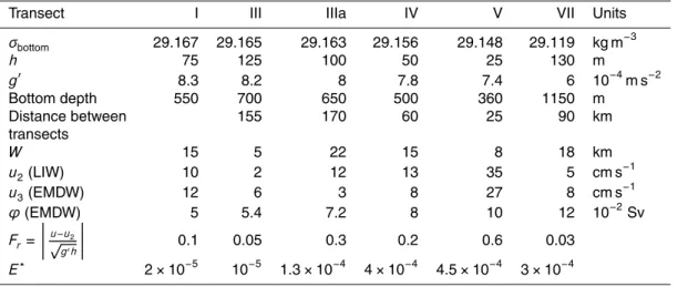
Table 2.Same as Table 1 but for the MATER IV cruise (Figs. 1 and 4).

Transect I III IIIa IV V VII Units

σbottom 29.167 29.165 29.163 29.156 29.148 29.119 kg m− 3

h 75 125 100 50 25 130 m

g′ 8.3 8.2 8 7.8 7.4 6 10−4m s−2

Bottom depth 550 700 650 500 360 1150 m

Distance between 155 170 60 25 90 km

transects

W 15 5 22 15 8 18 km

u2(LIW) 10 2 12 13 35 5 cm s−

1

u3(EMDW) 12 6 3 8 27 8 cm s−

1

ϕ(EMDW) 5 5.4 7.2 8 10 12 10−2Sv

F_r=

u−u2 √

g′_h

0.1 0.05 0.3 0.2 0.6 0.03

(28)

OSD

11, 2495–2532, 2014

a marine strait

Title Page

Tables Figures

◭ ◮

Back Close

Full Screen / Esc

Discussion

P

a

per

|

Discus

sion

P

a

per

|

Discussion

P

a

per

|

Discussion

P

a

per

Table 3.Theoretical estimates ofζ for the MATER II cruise (Figs. 1 and 3). Values are

com-pared with the approximate vorticitiesζ₀_∼U/W (which moreover sets the initial values of our

theoretical estimation) andζ=_hf h

∞−f (see text). The last two rows show theoretical estimates

ofΠandζ_ψ.

Transect I II III IV V VI VII Units

ζ 7 2.0 ₋1.5 ₋60.5 20.0 45.5 50.0 10−6s−1

u/W 7 10 1.2 ₋10 ₋30 5 8.5 10−6s−1

fh−h∞

h_∞ 0 25 16 −16 −58 25 66 10−

6 s−1

Π 8 7.0 7.5 5.0 19.5 9.0 6.0 10−7m−1s−1

(29)

OSD

11, 2495–2532, 2014

a marine strait

Title Page

Tables Figures

◭ ◮

Back Close

Full Screen / Esc

Discussion

P

a

per

|

Discus

sion

P

a

per

|

Discussion

P

a

per

|

Discussion

P

a

per

|

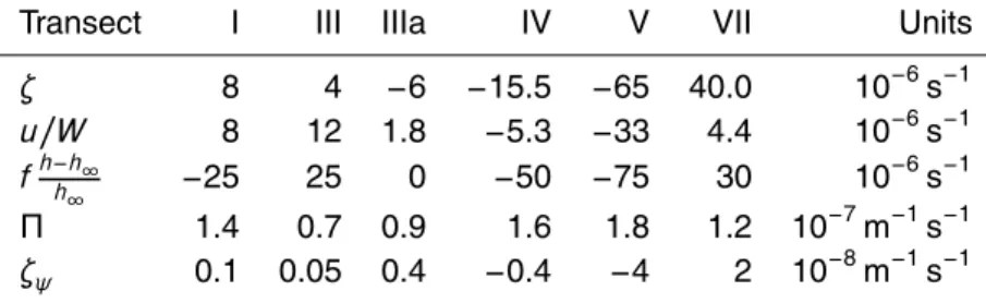
Table 4.Same as Table 3 but for the MATER IV cruise (Figs. 1 and 4).

Transect I III IIIa IV V VII Units

ζ 8 4 −6 −15.5 −65 40.0 10−6s−1

u/W 8 12 1.8 ₋5.3 ₋33 4.4 10−6s−1

fh−h∞

h_∞ −25 25 0 −50 −75 30 10

−6 s−1

Π 1.4 0.7 0.9 1.6 1.8 1.2 10−7m−1s−1

(30)

OSD

11, 2495–2532, 2014

a marine strait

Title Page

Tables Figures

◭ ◮

Back Close

Full Screen / Esc

Discussion

P

a

per

|

Discus

sion

P

a

per

|

Discussion

P

a

per

|

Discussion

P

a

per

Figure 1a.General map of the Sicily Channel: the channel length is_∼500 km, with two sills at

its eastern and western entrances (_∼550 and_∼350 m deep, respectively). Dots indicate the