A QoS Solution for NDN in the Presence of Congestion Control Mechanism

A QoS Solution for NDN in the Presence of

Congestion Control Mechanism

Abdullah

Alshahrani

Izzat

Alsmadi

Abstract—Both congestion control and Quality of Service (QoS) are important quality attributes in computer networks. Specifically, for the future Internet architecture known as Named Data Networking (NDN), solutions using hop-by-hop interest shaping have shown to cope with the traffic congestion issue. Ad-hoc techniques for implementing QoS in NDN have been proposed. In this paper, we propose a new QoS mechanism that can work on top of an existing congestion control based on interest shaping. Our solution provides four priority levels, which are assigned to packets and lead to different QoS. Simulations show that high priority applications are consistently served first, while at the same time low priority applications never starve. Results in ndnSIM simulator also demonstrate that we avoid congestion while operating at optimal throughputs.

Keywords—Named Data Networking; Quality of Service; Con-gestion Control

I. INTRODUCTION

Throughout the years, observation of todays Internet archi-tecture has shown that its usage has shifted from its original route sough in early design. In order to have a more adequate design for future Internet, the U.S. National Science Founda-tion [21] is funding the NDN project [19], which focuses on developing a Content-Centric architecture. In contrast to the host-centric architecture of IP networks, NDN allows users to request data without the need of referencing the server IP address. Therefore, the routers are responsible to find the data provider, relieving the user of complex configurations and making the data-hosting more flexible and network indepen-dent.

In NDN architecture, requests are called interests while data itself is named content. End-points that send interests are calledconsumersand end-points that provide contents are called producers. In this paradigm, an interest packet, which contains the name of the resource it requires, is replied by a single content packet, which also contains the resource name. Content packets always traverse the inverse path of the interests that triggered them. This characteristic can be translated as Property 1.

Property1:In NDN the sum of all interest packets that traverse a link in one direction is equal to the sum of all content packets that traverse the same link on the reverse direction. This property implies that hop-by-hop techniques are particularly interesting for NDN, because the flow of content packets is predictable (as shown in Fig. 1)

The technique proposed in [11] proposes a hop-by-hop congestion control mechanism for NDN that also relies on

Fig. 1: Content packets always travel the inverse path of interest packets in NDN

Property 1. This solution is based on the idea that controlling the interest packet rate in one direction can regulate the traffic of contents in the reverse direction. By shaping the outgoing interest rate to an optimal value, the incoming content rate is indirectly shaped to maximize the use of available bandwidth while minimizing the loss of content packets.

Besides congestion control concerns, NDN should offer the possibility of discerning among different service priorities. For instance, video streaming and gaming applications must be treated with more priority by routers than a regular download. Thus when co-existing, high-priority applications should be served faster than low-priority ones. In existing networks, this service is among one of the many features provided by Quality of Service (QoS) mechanisms. In other words, QoS techniques should offer to higher priority services higher throughput, shorter transmission delays, more availability and less jitter.

In this paper, we propose a practical hop-by-hop solution for QoS in NDN that can be integrated with the existing congestion control solution proposed in [11]. Our mechanism offers four priority levels, each one designed for a particular class of applications. Real-time traffic (higher priority apps) is always served first, guaranteeing high QoS; while low-priority services have a minimum QoS with no starvation. Results at ns-3 ndnSIM [13] simulator show that the proposed mechanism reaches optimal bandwidth usage with a negligible congestion. In addition, the solution offers a flexible QoS configuration, making it possible to change at will the way that routers treat different priorities.

The rest of the paper is organized as the following: Section II introduced relevant related papers. Next section introduced interest shaping congestion control. Main paper contribution is in next sections experiments and analysis. Paper is then concluded in section VI.

II. RELATEDWORK

Named Data Networking (NDN) [22] extended original project:(Content-Centric Networking (CCN),[23] as an alter-native architecture to classical IP-based Internet networking architecture. Unlike the former IP-based networking, NDN aims at uniquely identifying Internet content rather than users or hosts. This information-centric architecture is proposed to allow the Internet to accommodate usage scenarios that it is believed that IP-based architecture was not natively built to handle or accommodate such scenarios. For example, a popular page in the Internet can be redundantly saved and stored in different locations. The large volume of users’ traffic with such popular pages can be significantly reduced if the Internet architecture handles all those instances of similar content synonymously. Consumers or data requesters express their interests and routers exchange this traffic based on content name. Receivers or owners of this content send back requested content in the same-but reversed paths. The focus or scope of our paper; a user- or content-driven resources’-allocation network is an example of those usage scenarios. If the un-derlying architecture is a host-driven, it will be hard for such architecture to accommodate dynamically different bandwidth and resources for different applications coming from the same users or hosts. Their are two key elements in NDN, related to our paper scope. Those are stateful forwarding which enables transmitted packets to traverse the same, reversed, path of packet requests and second adaptive forwarding which enables routers ti change their future routing decisions based on current traffic and also consumers’ requests.

In the context of NDN and user-driven congestion controls [24] proposed a receiver-driven congestion algorithm to predict the location of desired content. For each packet, timeout is defined in their algorithm based on originating nodes. For each packet, the originating nodes are expected to list next data packets. As a result, each router can judge if they have those next packets or their destinations where ultimately the receiver can have a map for future packets and hence better manage or control traffic congestion. The idea of the involve-ment of receivers or consumers in smart or adaptive routing decisions is discussed also in similar other contributions (e.g. [28]). In this paper, authors proposed an Explicit Congestion Notification (ECN) based routing algorithm in which con-sumers can utilize network-wide range information to make smart routing decisions. [25] proposed an architecture for an adaptive routers’ multi-path forwarding algorithm based on NDN to accommodate in addition to traffic congestion, security problems and traffic failures. In order to minimize congestion, routers should try efficient routing algorithms to avoid the last resort of sending interests to all interfaces. Their algorithm is based on ranking router interfaces and sending interests to interfaces with highest ranks. Routing information and forwarding performance are the two main factors to consider in this ranking scheme. Their algorithm extended original algorithm in NDN prototype software implementation:CCNx

[26]. Upon a link failure, next-ranked interface will take the rank precedence.

In the same scope of NDN content adaptive forwarding, [27] proposed nCDN to enhance Content Delivery Network (CDN) based on NDN and allow NDN over UDP/TCP to utilize best features of NDN such as: Caching, multi-casting and stateful forwarding to reduce network congestion. Identical interests can be aggregated to optimize resources’ utilization.

Other QoS solutions have been proposed for NDN. In [14], the authors propose to include a data lifetime information on the NDN packet header. The lifetime tag at the packets are translated into the storage lifetime at Content Stores. This is implied into improvement of service availability for applications that emit larger lifetime packets.

In [6], IP differentiated services are used as a guideline to implement QoS in NDN. The authors propose the use of traffic classification and packet tagging at edge routers. The core routers offer a special treatment to packets with certain tags.

None of the previous solutions considered the traffic con-gestion issue. Therefore, we believe that this is the first mechanism that make use of the control congestion structure to provide QoS. Regarding the traffic congestion issue, there are several proposals of solutions. In [15], [16], the authors proposed a credit-based interest shaping scheme to control data traffic volume. Each flow is giving certain credits at a rate that is equal to the available downlink capacity divided by the number of bottlenecked flows. If the outgoing Interest rate for a flow exceeds the credit, the flows Interests will be dropped or delayed. Note that a content flow is defined as the packets bearing the same content name or prefix identified on the fly by parsing the packet headers. In [17], the authors proposed a rate-based hop-by-hop congestion control mechanism to shape the Interest rate that follows the same principles as the rate control mechanism for Available Bit Rate (ABR) in ATM networks [18] and the interest sending rate is computed as a function of the target flow queue occupancy.

In [11], a per-interface based Interest limit mechanism is used in which a router limits the rate in forwarding interest packets for each interface to prevent congestion and an in-terface becomes unavailable when it reaches its interest limit. The interest rate limit is based on link capacity and estimated requested packet size. This work is elaborated in Section III, since it is used as a basis for our QoS solution.

In [19], a fair share interest shaping (FISP) is proposed. In this solution, a content router decides whether to forward an interest immediately or delay it temporarily based upon the data queue sizes and the flow demands. Then it realizes fair bandwidth sharing among flows by having per-flow interest queues at an interface. Next, it uses a modified round robin scheduling mechanism for these per-flow interest queues (the deficit counter of the queue is decreased by the size of corresponding data after sending an interest).

These existing Interest shaping mechanisms assume that the link capacity is equally divided among the bottlenecked flows during congestion. They do not consider different pri-orities of various flows. An unloaded network can meet the

Fig. 2: Control congestion solution presented in [3]

needs of all applications and subscribers. However, the impor-tance of quality of service (QoS) increases during periods of congestion. In an overloaded network, it is vital to ensure the QoS of the important, delay-sensitive traffic (e.g., continuous uninterrupted multicast TV flows viewed by thousands), while less important and delay-tolerant traffic can be buffered or discarded.

The rest of our paper is structured as follows: Section II contains a description of related work. In Section III, we briefly explain the control congestion technique presented in [11], since we reused the same principles. Section IV describes our QoS solution for NDN. In Section V we present our results and make a qualitative analysis of the ideal configurations. Finally, we conclude our paper in Section VI.

III. INTERESTSHAPINGCONGESTIONCONTROL

In [11], the authors proposed a hop-by-hop interest shaping mechanism to cope with network congestion. As shown in Fig. 2, each router has an uplink and downlink bandwidth related to that hop, named b1 and b2 respectively. The interfaces at each side of the link receive interests that need to be sent out through that link (at ratesi1 for router 1 andi2 for router 2). In addition, returning contents arrive at rates c1 and c2. At router 1, interests are placed at the shaping queue at i1 rate. Then the shaper decides whether to limit or not the outgoing interest rate (named hereafter shaping rate or s1for router 1). The same occurs at router 2. In the NDN architecture, each interest packet sent through a hop must be replied with exactly one content packet (cf. Property 1). Therefore, any device interface will send the same number of interests o contents it receives (except if there is packet loss). So if we measures1 andc2in number of packets per second, s1 should be equal to c2, meaning that controlling only the interest rate (s1) implies in indirectly controlling the content rate (c2). In that way, wisely choosing the shaping rate leads to an optimal use of the bandwidth with minimal congestion. For instance, suppose that at router 1 we measure thes2rate, and it occupies10%of the b2 bandwidth. Thens1 can be chosen so that c2 occupies the 80% left ofb2, reaching a full usage with no congestion. That same logic applies to router 2. The adaptation ofs1 and

Fig. 3: Implementing priorities

s2occurs instantly. Actually,s1ands2 may assume less than optimal values to have some slack for burstiness. In [11], the shaping rate is chosen according to a theoretical analysis of the congestion problem at a single hop. First, the authors define a range for shaping rates, with maximum and minimum shaping rates. This range depends on the instant values of b1,b2, i1, i2, and the ratios between interests and content sizes. In real-world scenarios, all these data can be measured at any instant. Then, actual shaping rate s1 is chosen inside this range by confronting the observed instant shaping rate s2 (called here obs s2) with the minimum expected shaping rate s2 (called here expmins2). Eq. 1 gives the actual shaping rates1.

s1= mins1+ (maxs1−mins1)(1− obs s2 expmin s2)

2 (1)

where obs s2 expmin s2 ≤1

As shown in Eq. 1, the greater the ratio between obs s2 and expmin s2, more s1 approaches the minimum value (mins1). In other words, highers2 rates occupy more down-link bandwidth (b2 in Fig. 2), so c2 rate should be reduced to avoid congestion. The shaper alone does not guarantee congestion avoidance. Consumers must be noticed when their interest rates are too fast, otherwise there are too much packet losses. Therefore, each dropped packet in the shaper queue generates a negative acknowledgment (NACK) message to the consumer. Thus, it reduces the interest rate to match the instant shaping rate. Results [11] show that this solution achieves high bandwidth use for both downlink and uplink while avoiding congestion conflicts, thus, minimizing packet loss. In Section III, this solution is extended to provide QoS, maintaining the advantages of congestion control while offering the user different QoS options.

IV. IMPLEMENTATION OFQOSINNDN

In the control congestion solution [11], only interest pack-ets are shape-able: content packpack-ets skip the shaper queue. Shaping only interest packets is effective against traffic con-gestion because controlling the shaping rate means an indirect control of the returning content rate. Notice that this is only valid in NDN due to Property 1. Our solution also assumes that Property 1 holds true.

A. Priority Levels

In order to offer QoS, our solution offers 4prioritylevels. Applications can pro-grammatically choose the priority of the packets it sends, as needed:

• Priority 0: This priority is assigned to background services that have no need of shorter transmission delays neither higher data throughput.

• Priority 1: Best effort. Should have a better quality of service than priority 0.

• Priority 2: Excellent effort. Assigned to critical ap-plications that need better quality but that cannot interfere with priority 3 services.

• Priority 3: assigned to real-time services (e.g. stream-ing) or network control services.

Having only 4 priority levels makes the classification meaningful. In other words, that the difference of treatment (difference of QoS) between one priority level and the next one is significant. In Section IV, we show that the difference of treatment given to different priorities is configurable. There-fore, if in practice one observes that priority 2 services should have more throughput than it had in a previous time, it is just a matter of updating the router configurations. The priority levels must be included in the header of interest packets. NDN headers are currently defined as a sequence of Type-Length-Value definitions. Interest packets have special types, such as Nonce, InterestLifeTime and Selectors. We propose to include the priority levels as a new special type (using one of many available type values). Remember that contents are not shapeable, thus only half of the packets need this extra parameter. Additionally, packets without this extra field might be considered as having priority 0, which ultimately reduce the overhead.

B. Implementation

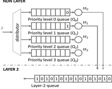
Regarding the implementation of the priority levels, the concept of congestion control with interest shaping is reused. Instead of implementing a single shaper (and a single queue) for each interface, 4 sets of shapers and queues must be present. Each set is assigned to a different priority level, as shown in Fig. 3. This solution concerns only outgoing packets. Incoming packets are not shapeable as in [original]. Also, con-tent packets arriving from other interfaces are directly placed at the layer-2 queue (The below layer, e.g. Ethernet). On the other hand, interest packets are given to a distributor. The distributor places the interest packets on the queue corresponding to the priority level set on the packet header. Queue sizes are set to a maximum value. The queue management policy used in our implementations is drop-tail, meaning that if the queue

size is below the maximum value, it pushes the packet into it, otherwise it drops it. When a drop occurs, a NACK is sent back to the source, in order to reduce the consumer throughput. Interest packets placed on the queue wait to be served according to their sub-shaping rate. Each queue has a different sub-shaper rate, named hereafter ss0, ss1, ss2 and ss3 (ssx is the shaping rate of priority level x). In order to choose the optimal sub-shaper rates, first the main shaping rate s is calculated from Eq. 1, exactly as described in [11]. Once s is defined, the sub-shaping rates are calculated using Eq. 2:

s=ss0+ss1+ss2+ss3 (2)

As it can be seen from Eq. 2, the sum of sub-shaping rates is equal to the main shaping rate. It means that, even with multiple priority queues, the main shaping rate targets optimal value for congestion control.

In order to differentiate the priority levels, giving more throughput to higher levels, ss0 ,ss1 ,ss2 andss3 must be chosen accordingly to Eq. 3:

ss3> ss2> ss1> ss0 (3)

With only Eq. 2 and Eq. 3, the sub-shaping rates cannot be calculated. Thus, we correlate all the sub-shaping rates using Eqs. 4-7:

ss3=w3·s (4)

ss2=w2·s (5)

ss1=w1·s (6)

ss0=w0·s (7)

Wherewxis called weight. From Eqs. 4-7, one can deduce that the sum of weights result in 1, as shown in Eq. 8:

1 =w0+w1+w2+w3 (8)

It means that each weight is the percentage of the main shaping rate allocated for that sub-shaping rate. Therefore, choosing the weights allows the network engineer to define how much throughput will be given to each priority level. It must be noticed thatw0has actually fixed value, once the other weights are chosen (due to Eq. 7).

It is not the purpose of this paper to discuss the better configurations of weights. However, Eq. 3 forces higher prior-ity levels to have higher sub-shaping rates, guarantying higher QoS to these services. In Section IV, results show that our solution works with different choices of weights. Additionally, it is easy to use this methodology to define any number of priorities, if required. In this paper, we only consider 4 priority levels.

C. Dynamic weights

The sum of weights shown in Eq. 8 expects that all sub-shaper queues have packets, i.e. packets tagged with all priorities are being sent through that interface. Therefore, all the weights will have values different than 0 and will thus have a share on the main shaping rate. However, there are cases where not all priority levels are going to be present.

For instance, assume that only services with priority level 0 are using a specific router. Assume also that the network engineer has setw1to2,w2to4andw3to8. In this case,N+1

level services would have twice throughput as N services.

In that case, if we keep the sharing of the main shaping rate as shown in Eqs. 4-7, those priority level 0 services would use only6.66%of the main shaping rate. Since other priority level services are not present, there would be a waste of bandwidth. In order to always make optimal bandwidth usage, Eqs. 4-7 should be slightly changed to Eqs. 9-12:

α0=w0 if Q0 is not empty, otherwise 0 (9)

α1=w1 if Q1 is not empty, otherwise 0 (10)

α2=w2 if Q2 is not empty, otherwise 0 (11)

α3=w3 if Q3 is not empty, otherwise 0 (12)

Which can be applied to Eqs 13-17:

1 =α0+α1+α2+α3 (13)

ss0=α0·s (14)

ss1=α1·s (15)

ss2=α2·ss0 (16)

ss3=α3·ss0 (17)

According to Eqs 9-17, the main shaping rate is now shared only between priority level services that are alive. For instance, if only priority level 0 service is alive, Q1,Q2 and Q3 will be empty, thus a1,a2 anda3 should be equal to 0, while a0 should be equal to 1. Therefore, w0 is equal to 1 (100%), meaning that ss0 is equal tos itself. In other words, priority level 0 services take the whole throughput.

It must be noticed that with four queues, andQ0,Q1,Q2 and Q3 assuming two possible states (empty or not empty), there are 16 possible cases where our solution theoretically makes optimal use of bandwidth. For those our solution theoretically makes optimal use of bandwidth.

Fig. 4: Some scenarios may cause instability

D. Stabilization

As described in the previous subsection, the sub-shaping rates can assume different values dynamically. However with rates changing instantly, the system may reach undesirable states due to instability.

For instance, suppose that the weights are set tow1 to2, w2to4andw3 to8. Suppose also that consumers are sending only packets with priority level 0 and 1. Thus, sub-shaping rate ss0 should be 33% of the main shaping rate and ss1 should be the double: 66% (from Eqs. 9-17).ss2 andss3 would be equal to zero. Now suppose that the interest rates are equal to the shaping rates and that each queue has only one packet, as shown in Fig. 4.

When theQ0is fed at the same rate asss0rate, the queue size oscillates from 0 to 1, never reaching more than 1. In other words, the shaper consumes the same number of interest packets sent by the consumer. The same behavior occurs toQ1. Simulations showed that this scenario may quickly become one of the below scenarios:

1) Q0size equal to1andQ1size equal to1. In this case, the sub-shaping rates assume the expected values. 2) Q0size equal to1andQ1size equal to0. It happens

sincess1is faster thanss0,Q1may be served before Q0. In this case, Q0 will have 100% of the main shaping rate.

3) Q0 size equal to 0 and Q1 size equal to 1. In this case, Q1 will have100%of the main shaping rate.

It is clear that scenarios 2 and 3 lead to incorrect shaping rates, violating Eqs.4-7. Additionally, Scenario 2 violates Eq. 3. If these scenarios occur frequently, in average, the sub-shaping rates ss0 and ss1 will be 50% of main shaping rate each, leading to an undesired QoS.

In order to add stability to this system, we consider that a queue is empty only when it has been empty after a while. It

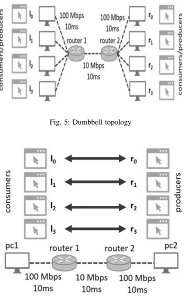
Fig. 5: Dumbbell topology

Fig. 6: Baseline topology

implies that the sub-shaping rates resist changing to transitional states, improving stability. It must be noticed that, this delay does not apply to the inverse logic: empty queues that are filled with packets are instantly served accordingly with its sub-shaping rate. For instance, in the example of Fig. 5, if a service with priority level 3 arrives, the system automatically shares the main rate among ss0,ss1 andss3 (which assume the values of 14.28%,28.57% and57.14%).

E. Software implementation

This solution was implemented using the ndn-extension of ns-3 simulator. It is an event-driven simulator where events such as packet sending can be scheduled programmatically at the desired simulation time. Each event triggers a function that treats it when in occurs.

In order to code a shaper, we reuse the code presented at [20]. Then, each time an outgoing packet arrives at a NDN device interface, the distributor places it on the right queue. If that queue is empty, a send event for that queue is scheduled.

Fig. 7: Interest rate vs time (scenario 1)

Each time a send event triggered, the main shaping rate is calculated as well as all sub-shaping rates. Therefore, update frequency of sandssx is equal to the shaping rates.

For the incoming packets arriving at the interface, the values of obss2 andE(mins2)are updated as well. It means that at simulation all values are updated instantly.

V. SIMULATIONRESULTS

Two main topologies were defined in order to extract the results: a baseline topology (see Fig. 6) and a dumbbell topology (see Fig. 7). The baseline topology consists of two routers (router 1 and router 2) and two computers (pc1 and pc2). The link between routers has a 10 Mbps bandwidth while the other links have 100 Mbps bandwidths. All links have a 10ms delay. Up in the application layer, pc1 has four consumer applications (named p0, p1, p2 and p3) with priority levels 0, 1, 2 and 3. All consumers use the AIMD (Additive-Increase, Multiplicative-Decrease) algorithm, due to its congestion avoidance nature. Each consumer searches for a content prefix defined at a different producer (the prefixes are /p0, /p1, /p2 and /p3).

The second topology also contains two routers, but it contains four computers at each side. Each computer has a consumer application running at a unique priority level. li is the application running on the left side while ri is the application running on the right side, where ialso represents the priority level. li consumes data from ri, andri consumes data from li (i goes from 0 to 3) For all scenarios (except explicitly said otherwise), the weights are set as: w3 is equal to 8, w2 is equal to 4 andw1 is equal to 2. In this case, the sub-shaping rate for packets with priority levelN+ 1is twice as fast as the sub-shaping rate for packets with priority level N. If services from all priority levels are alive, the sub-shaping rates are distributed as show in Eq. 18-21:

ss3=s×0.5333 (18)

ss2=s×0.2666 (19)

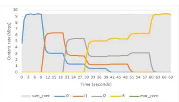
Fig. 8: Content rate vs time (scenario 1)

ss1=s×0.1333 (20)

ss0=s×0.0666 (21)

To extract the results, an ndnSIM tracer is used. It shows periodically the exponentially weighted moving average (EWMA) of all interests and contents flowing through each interface. This module is modified so it also shows QoS information. For all simulations, the main shaping rate was multiplied by 0.98 (named headroom) to make 2% room for unattended bursts. Additionally, all simulations were repeated at least 10 times to obtain deviation information. All shaper queues and layer-2 queue were set to have at most60packets. In the next subsections, we present simulation results for several scenarios. The scenario described in Subsections A, B, C and D use the baseline topology while the others use the dumbbell topology. The communication for scenario 1 is unidirectional, meaning the left side applications are only consumers. All the other scenarios use bidirectional communi-cation, meaning that all apps are both consumer and producers.

A. Scenario 1: Priorities dynamics

The first scenario aims at simulating a baseline topology, exactly as shown at Fig. 6. All producers payloads are set to 1000B. Contents have a 32B header (leading to 1032-sized packets). Consumers send interest packets with an average size of 26B. Applications p0, p1, p2 and p3 start and stop operating at different times, in order to show the shapers dynamics. From time 0s to 10s only application p3 is alive. P3 is later shut down at time 40s. p2 is turned on from time 10s until 70s. P1 is turned on from time 20s until 60s. P0 is alive from time 30s until 50s. Fig. 7 shows the sub-shaping rates for all four applications during a 70-second simulation. The green lines represent the maximum achievable rates for interest and contents. All throughputs are traced at the NDN layer, meaning that the bandwidth at this layer is not the full10Mbps (due to the overhead of link layer). The maximum throughput at NDN layer can be calculated from Eq. 22:

Link layer throughput efficiency×bandwidth×headroom (22)

Where the link layer adds only 2 extra header bytes. Therefore, for content packets (1032 bytes long) the maximum

Fig. 9: Interest rate vs time for left side (scenario 5)

Fig. 10: Content rate vs time for left side (scenario 5)

content rate is9.7810M bps. Since the prefixes increase with time (e.g. from /p0/1, /p0/2, , to /p0/10) the size of the header of both interest and content packets get larger. For 1033-byte long content packets, the content rate is9.7905M bps. In order to generate these content rates, the maximum interest rates are 0.2464 M bps (for 26 B) and 0.2558 M bps (for 27 B), obtained from Eq. 23:

max.content rate×interest packet size

content packet size (23)

The sum of sub-shaping rates is shown as the gray area. As it can be seen from Fig. 7, the sum of rates approaches the maximum interest rates described earlier (green line). Fig. 8 shows the returning content rate. The incoming content rate (blue line) also approaches the maximum content rate (green line), showing that our solution achieves optimal bandwidth usage.

As shown in Fig. 7 and Fig. 8, the saw behavior of rates is due to the AIMD consumers. Each time that a shaper queue drops a packet, a NACK is sent to the consumer, which causes a multiplicative decrease of its window size. Later, the consumer increases additively the window size. This decrease-increase behavior generates saw waves.

The proportions of sub-shaping rates in relation to the sum of interest rates (in Fig, 7) respect the configurations specified

Fig. 11: Interest rate vs time for left side (scenario 6)

at Section IV. For instance, at time 35s (when all applications are alive), p3 obtains 0.1291M bpsout of0.25M bps, which gives 53.25% as expected from Eq.18. P2, P1 and P0 have rates equal to 0.066 M bps, 0.035 M bps and 0.018 M bps, whose percentages are26.66%,13.33%,6.25%, also matching Eqs. 19-21.

It must be noticed that at transition times (i.e. in every seconds), the content rates may have valleys (Fig. 8). It may happen because when one rate decreases and another one increases, the decrease is multiplicative while the increase is additive. Thus, the sum of rates tends to decrease faster than increase until it reaches a stable state.

B. Scenario 2: Randomized packet size

In this scenario, the baseline topology is used. However, the consumers reply with random payloads, instead of using a fixed-size (1000 bytes). The payloads vary randomly from 600 bytes to 1400 bytes. In addition, the four applications are alive during the whole simulation time (20 seconds). In this and for all the subsequent scenarios the transmission is bidirectional. In other words, the computer on the right side has also four consumer applications (r0, r1, r2 and r3) that are sending interests towards the left side (similarly to the dumbbell topology).

Table 1 shows the results for scenario 2, 3 and 4. As shown, the left side applications (l0 to l3) respect the sharing of the main shaping rate (represented by the sum row) specified at Eqs. 18-21. The same occurs for right side applications.

As shown in Table 1, the actual content rate for this scenario (for both left and right sides) matches the maximum rate. Since the maximum content rate depends on the protocol efficiency, which depends on the payload size, this maximum value is slightly different from the scenario 1. It must be calculated from the average payload is 1000B, we calculate those maximum values from Eqs 22-23.

It must be noticed that even when both sides are sending interests the system achieves optimal bandwidth usage respect-ing the priority weights.

Fig. 12: Content rate vs time for left side (scenario 6)

C. Scenario 3: Asymmetric Size Ratio

In this scenario, the payload is also modified: producers on the right side send 500B-payload packets while producers on the left side still send 1000B-payload packets. Table 1 shows the interest and content rates for both sides.

The results show that the proportions of sub-shaping rates in comparison with the main shaping rate (sum) respect Eqs. 18-21. The content rate also reaches optimal use (almost equal to maximum value). The 1000B maximum is the same as the one calculated in Scenario 2, where the average payload has 1000 bytes. However, the maximum rate for the 500-bytes payload size is slightly different, because the protocol overhead charges more on smaller payloads.

In addition to that, the interest rate for left side has increased. This behavior is expected because reducing the payload to 500B (in average, half of the previous scenario) allows the double of packets to flow in that link. It implies thus in almost doubling the shaping rate (as shown in Table 1). Additionally, the maximum values here are the ones that appear in [11].

D. Scenario 4: Asymmetric Link Bandwidth

The purpose of this scenario is to validate the proposed technique on routers with asymmetric bandwidth, meaning that downlink and uplink have different throughputs. In this case, baseline topology with bidirectional communication is used (4 apps on each side). The link from router 1 to router 2 is set to 1Mbps while the reverse link is set to 10Mbps. Table 1 also present the results for this case. As we can see:

The 10Mbps link present similar results to the random packet size scenario. However, the content rate sum is greater than previous cases because the interest rates for that link occupy less bandwidth (only 0.0173 Mbps) since their contents are on the reverse 1Mbps link. In addition, the content rate sum matches with the value presented in [11].

The reverse link is under 1Mbps and its sum corresponds to the value presented at [11]. It is important to notice that even for the smaller bandwidth the priority levels are respected.

TABLE I: Interest and Content rates (in Mbps) for scenarios 2, 3 and 4

Senarios

Random packet size Asymmetric size ratio Asymmetric link bandwidth

Interest rate Content rate Interest rate Content rate Interest rate Content rate

l0 0.0170±0.0002 0.6820±0.0171 0.0331±0.0003 0.6717±0.0087 0.0006±0.001 0.0158±0.023

l1 0.0340±0.0003 1.3341±0.0242 0.0661±0.0007 1.3382±0.016 0.002±0.0011 0.0904±0.0248

l2 0.0679±0.0007 2.6688±0.0348 0.1313±0.0021 2.6429±0.0277 0.0047±0.0003 0.1935±0.0095

l3 0.1213±0.0024 4.7553±0.0696 0.1752±0.0084 3.5001±0.1381 0.0098±0.0001 0.3958±0.0044

Sum 0.2404±0.0031 9.4404±0.0785 0.4058±0.0112 8.153±0.1617 0.0173±0.001 0.6956±0.0295

M ax 0.2479(from Eq.23) 9.52(from Eq. 22) 0.39(from Eq. 23) 8.34(from Eq. 22) 0.017(from eq. 23) 0.7195(from [3])

r0 0.0171±0.0001 0.6673±0.0149 0.0166±0.0002 0.6619±0.0089 0.0174±0.0002 0.6911±0.0059

r1 0.0341±0.0003 1.3465±0.0247 0.0332±0.0002 1.3064±0.0144 0.0347±0.0003 1.3669±0.019

r2 0.0681±0.0006 2.6728±0.0252 0.066±0.0005 2.5949±0.0251 0.0631±0.0021 2.4813±0.084

r3 0.1224±0.0011 4.7852±0.0461 0.1214±0.0009 4.7506±0.0328 0.1329±0.0033 5.1872±0.074

Sum 0.2416±0.0020 9.4718±0.0254 0.2374±0.0015 9.3139±0.0122 0.2483±0.0021 9.7267±0.0034

M ax 0.2479(from Eq.23) 9.52(from Eq. 22) 0.236(from Eq. 23) 9.3736(from [3]) 0.246(from Eq. 23) 9.7744(from [3])

Fig. 13: Average interest rate vs Maximum queue size (sce-nario 6)

E. Scenario 5: Homogeneous RTT

From this scenario on, we use the dumbbell topology. Applications have different lifetimes and we change start and stop times using a 10 seconds step. Fig. 11 and Fig 12 show the interest and content rate for the applications on the right side (left side applications are omitted due to similarity of results).

As shown in Fig. 9,l3starts at 0s and stop at 50s.l2starts at 20s and live through the rest of simulation time.l1lives from 10s to 30s whilel0 lives from 10s to 40s. Since interest rates are smaller than content rates, oscillations are more visible at Fig. 12. As expected, even in the dumbbell topology, the sub-shaping rates have the right proportions.

TABLE II: Interest and content rates for scenario 7

Interest Rate Content Rate

l0 0.0253±0.0003 0.9986±0.0205

l1 0.0506±0.0003 1.9892±0.0127

l2 0.0761±0.0004 2.9915±0.0189

l3 0.0892±0.0008 3.5085±0.0326

Sum 0.2413±0.0003 9.4879±0.0038

M ax 0.2479(from Table 1) 9.5231(from Table 1)

r0 0.0253±0.0003 0.9986±0.0205

r1 0.0506±0.0003 1.9892±0.0127

r2 0.0761±0.0004 2.9915±0.0189

r3 0.0892±0.0008 3.5085±0.0326

Sum 0.2413±0.0003 9.4879±0.0038

M ax 0.2479(from Table 1) 9.5231(from Table 1)

F. Scenario 6: Heterogeneous RTT

This scenario aims at testing our solution in heterogeneous round-trip times (RTT). For that, links connected to computers that hostl1andl3are now set 20ms instead of 10ms. Fig. 13. and Fig. 14 show the interest and content rates for the right side (remember that right side applications are communicating with those in left side).

As shown in both figures, the behavior is similar to the ones in scenario 5, demonstrating that heterogeneous RTT have no impact on this solution. It must be noticed that without the stabilization technique described in Section III, results would show an unstable system.

G. Scenario 7: Custom priority

In scenario 7, we apply other values for w1, w2 and w3 in order to test the flexibility of our solution. In the results presented Table 2, w1 is equal to2,w2 is equal to3 andw3 is equal to 4, reducing the ratios used in previous scenarios.

For both sides, the interest and content rates respect the proportion 1 to2 to3 to4. It must be noticed that even with other weights, the achieved rates correspond to the ones show in Table 1.

H. Scenario 8: Queue sizes

The last scenario aims at evaluating the ideal queue size for all priority levels. Fig. 23 shows the average interest rate vs maximum queue size for priority levels 0, 1 and 2; while Fig. 24 show it for priority level 3. The deviations are the bars at some points in the line. The ideal interest rate for each priority

level is also shown (the ideal rate is the rate predicted from the Table 1, considering any functional scenario, for instance scenario 2).

Shorter queues (below size 20) do not reach the ideal rate. This is especially visible forl2andl3, since they usually have higher rates. This effect happens due to the fact that shorter queues are more prone to send NACKs (they can easily drop packets).

On the other hand, the deviation bars show that for lower priorities (l0 and l1), larger queues (150) tend to have more deviation for the interest rates. It happens mainly when the sub-shaping rates are transitioning (as Fig. 19): longer queues will take more time to send NACKs and therefore the AIMD consumer will synchronize later.

Higher priority services always get faster shaping rates, which produce NACKs more easily. Thus, the higher devia-tions appear for p3.

VI. CONCLUSION

In this paper, we presented a mechanism that offers QoS on top of a congestion control solution. The hop-by-hop interest shaper is improved to use 4 sub-shapers in order to provide differentiated QoS to 4 priority levels. Results showed that higher priority applications have higher throughputs, while lower priority applications never starve. Our solution reacts instantly and dynamically to any configuration of requests, always using optimal bandwidth (even in cases where all not all priorities exist). Several simulations with complex scenarios have emphasized the validity of the proposed method.

REFERENCES

[1] Abdel-Hadi, A., and Clancy, C. (2014, February). A utility proportional fairness approach for resource allocation in 4G-LTE. In Computing, Networking and Communications (ICNC), 2014 International Conference on (pp. 1034-1040). IEEE.

[2] Abdel-Hadi, A., and Clancy, C. (2013, September). A robust optimal rate allocation algorithm and pricing policy for hybrid traffic in 4G-LTE. In Personal Indoor and Mobile Radio Communications (PIMRC), 2013 IEEE 24th International Symposium on (pp. 2185-2190). IEEE. [3] author = Ingo Ltkebohle Itu, R. (2008). ITU-R M. 2135: Guidelines for

evaluation of radio interface technologies for IMT-Advanced.

[4] Oh, J., and Han, Y. (2012, September). Cell selection for range expansion with almost blank subframe in heterogeneous networks. In Personal Indoor and Mobile Radio Communications (PIMRC), 2012 IEEE 23rd International Symposium on (pp. 653-657). IEEE.

[5] Richter, F., Fehske, A. J., and Fettweis, G. P. (2009, September). Energy efficiency aspects of base station deployment strategies for cellular networks. In Vehicular Technology Conference Fall (VTC 2009-Fall), 2009 IEEE 70th (pp. 1-5). IEEE.

[6] Wireless Systems Research Lab, Hitachi America Ltd, Cellular Network Topology Toolbox Implementation Documentation,

http://www.ltehetnet.com/sites/default/files/NetworkToolBox Documentation.pdf,2014. [7] Chinipardaz, M., Rasti, M., and Nourhosseini, M. (2014, September). An

overview of cell association in heterogeneous network: Load balancing and interference management perspective. In Telecommunications (IST), 2014 7th International Symposium on (pp. 1250-1256). IEEE. [8] Ghosh, A., Mangalvedhe, N., Ratasuk, R., Mondal, B., Cudak, M.,

Visotsky, E., and Dhillon, H. S. (2012). Heterogeneous cellular networks: From theory to practice. Communications Magazine, IEEE, 50(6), 54-64. [9] Fehske, A., Fettweis, G., Malmodin, J., and Biczok, G. (2011). The global footprint of mobile communications: The ecological and economic perspective. Communications Magazine, IEEE, 49(8), 55-62.

[10] Blume, O., Eckhardt, H., Klein, S., Kuehn, E., and Wajda, W. M. (2010). Energy savings in mobile networks based on adaptation to traffic statistics. Bell Labs Technical Journal, 15(2), 77-94.

[11] Wang, Y., Rozhnova, N., Narayanan, A., Oran, D., and Rhee, I. (2013, August). An improved hop-by-hop interest shaper for congestion control in named data networking. In ACM SIGCOMM Computer Communica-tion Review (Vol. 43, No. 4, pp. 55-60). ACM.

[12] Zhang, L., Afanasyev, A., Burke, J., Jacobson, V., Crowley, P., Pa-padopoulos, C., and Zhang, B. (2014). Named data networking. ACM SIGCOMM Computer Communication Review, 44(3), 66-73. Chicago [13] Mastorakis, S., Afanasyev, A., Moiseenko, I., and Zhang, L. (2015).

ndnSIM 2.0: A new version of the NDN simulator for NS-3. Technical Report NDN-0028, NDN. Chicago

[14] Wu, T. Y., Lee, W. T., Duan, C. Y., and Wu, Y. W. (2014). Data Lifetime Enhancement for Improving QoS in NDN. Procedia Computer Science, 32, 69-76.

[15] Oueslati, S., Roberts, J., and Sbihi, N. (2012, March). Flow-aware traffic control for a content-centric network. In INFOCOM, 2012 Proceedings IEEE (pp. 2417-2425). IEEE.

[16] Carofiglio, G., Gallo, M., and Muscariello, L. (2012, August). Joint hop-by-hop and receiver-driven interest control protocol for content-centric networks. In Proceedings of the second edition of the ICN workshop on Information-centric networking (pp. 37-42). ACM. Chicago

[17] Floyd, S. (1994). TCP and explicit congestion notification. ACM SIGCOMM Computer Communication Review, 24(5), 8-23.

[18] Moret, Y., and Fdida, S. (1997, November). ERAQLES an efficient explicit rate algorithm for ABR. In Global Telecommunications Con-ference, 1997. GLOBECOM’97., IEEE (Vol. 2, pp. 801-805). IEEE. Chicago

[19] Zhang, F., Zhang, Y., Reznik, A., Liu, H., Qian, C., and Xu, C. (2014, August). A transport protocol for content-centric networking with explicit congestion control. In Computer Communication and Networks (ICCCN), 2014 23rd International Conference on (pp. 1-8). IEEE. Chicago

[20] https://github.com/wygivan/ndnSIM [21] https://github.com/wygivan/ndnSIM

[22] Zhang, L., Estrin, D., Burke, J., Jacobson, V., Thornton, J. D., Smetters, D. K., and Abdelzaher, T. (2010). Named data networking (ndn) project. Relatrio Tcnico NDN-0001, Xerox Palo Alto Research Center-PARC. Chicago

[23] Jacobson, V., Smetters, D. K., Thornton, J. D., Plass, M. F., Briggs, N. H., and Braynard, R. L. (2009, December). Networking named content. In Proceedings of the 5th international conference on Emerging networking experiments and technologies (pp. 1-12). ACM. Chicago

[24] Saino, L., Cocora, C., and Pavlou, G. (2013, June). Cctcp: A scalable receiver-driven congestion control protocol for content centric network-ing. In Communications (ICC), 2013 IEEE International Conference on (pp. 3775-3780). IEEE.

[25] Yi, C., Afanasyev, A., Wang, L., Zhang, B., and Zhang, L. (2012). Adaptive forwarding in named data networking. ACM SIGCOMM computer communication review, 42(3), 62-67.

[26] http://blogs.parc.com/ccnx/

[27] Jiang, X., and Bi, J. (2014, April). nCDN: CDN enhanced with NDN. In Computer Communications Workshops (INFOCOM WKSHPS), 2014 IEEE Conference on (pp. 440-445). IEEE. Chicago

[28] Zhou, J., Wu, Q., Li, Z., Kaafar, M. A., and Xie, G. (2015, June). A proactive transport mechanism with Explicit Congestion Notification for NDN. In Communications (ICC), 2015 IEEE International Conference on (pp. 5242-5247). IEEE.