QUADRATIC BI-LEVEL PROGRAMMING PROBLEM BASED ON FUZZY GOAL PROGRAMMING APPROACH

(1)

International Journal of Software Engineering & Applications (IJSEA), Vol.2, No.4, October 2011

DOI : 10.5121/ijsea.2011.2405 41

Surapati Pramanik

1

and Partha Pratim Dey

2

1

Department of Mathematics, Nandalal Ghosh B.T. College, Panpur, P.O.-Narayanpur, District - North 24 Parganas, Pin Code-743126, West Bengal, India

sura_pati@yahoo.co.in 2

Patipukur Pallisree Vidyapith, 1, Pallisree Colony, Patipukur, Kolkata-700048, West Bengal, India

parsur.fuzz@gmail.com

A

BSTRACT

This paper presents fuzzy goal programming approach to quadratic bi-level programming problem. In the model formulation of the problem, we construct the quadratic membership functions by determining individual best solutions of the quadratic objective functions subject to the system constraints. The quadratic membership functions are then transformed into equivalent linear membership functions by first order Taylor series approximation at the individual best solution point. Since the objectives of upper and lower level decision makers are potentially conflicting in nature, a possible relaxation of each level decisions are considered by providing preference bounds on the decision variables for avoiding decision deadlock. Then fuzzy goal programming approach is used for achieving highest degree of each of the membership goals by minimizing deviational variables. Numerical examples are provided in order to demonstrate the efficiency of the proposed approach.

K

EYWORDS

Bi-level programming, Fuzzy programming, Fuzzy goal programming, Multi-objective Quadratic programming, Quadratic bi-level programming

1. I

NTRODUCTION

In this paper, we consider quadratic bi-level programming problem (QBLPP). QBLPP consists of a single decision maker namely upper level (first level) decision maker (ULDM) with single objective at the upper level and a single decision maker namely lower level (second level) decision maker (LLDM) with single objective at the lower level. The objective function of each level decision maker (DM) is quadratic in nature and the constraints are linear functions. The execution of decision is sequential from upper level to lower level. Each level DM independently controls only a set of decision variables. The decision of ULDM is affected by the reaction of the LLDM due to dissatisfaction with the decision of the ULDM. Therefore, decision deadlock arises frequently in the hierarchical organization in the decision-making situation.

(2)

42 MLPP by using tolerance membership functions. Shih et al. [5], Shih and Lee [6] extended Lai’s concept by introducing non-compensatory max-min aggregation operator and compensatory fuzzy operator respectively for MLPP. Sakawa et al. [7] developed interactive fuzzy programming for MLPP. Sinha [8, 9] presented alternative multi-level programming based on fuzzy mathematical programming. Arora and Gupta [10] presented interactive fuzzy goal programming approach for linear BLPP with the characteristics of dynamic programming. Satisfactory solution is derived by updating the satisfactory degree of the decision makers with the consideration of overall satisfactory balance between both the levels. A bibliography of references on bi-level programming as well as multi-level programming in both linear and nonlinear cases, which is updated biannually, can be found in the work of Vicente and Calamai [11].

Non-linear BLPP has been addressed in [12-13]. Edmund and Bard [13] discussed nonlinear bi-level mathematical problems in 1991. In contrast to BLPPs, nonlinear BLPPs [14, 15] have not been discussed extensively. Malhotra and Arora [16] developed an algorithm for solving linear fractional bi-level programming problem (LFBLPP) based on preemptive goal programming. Sakawa & Nishizaki [17-18] used interactive fuzzy programming for solving LFBLPP both in crisp and fuzzy environment. Calvete and Galé [19] studied optimality conditions for LFBLPP. Ahlatcioglu and Tiryaki [20] developed two interactive fuzzy programming algorithms for decentralized two-level linear fractional programming problem by using the technique of multi-objective linear fractional programming problem due to Chakraborty and Gupta [21], and Charnes and Cooper [22]. Mishra [23] discussed weighting method for LFBLPP by using analytical hierarchy process [24]. However, the solution obtained by Mishra’s approach [23] is the solution of the individual best solution of the ULDM or the LLDM.

It is worth mentioning that quadratic problems arise directly in applications related to least-square regression with bounds or linear constraints, central economic planning, robust data fitting, input-allocation problem, transportation, facility locations, traffic assignment problem, portfolio optimization, etc. QBLPP has been studied in [25- 30] Vicente et al. [27] introduced two descent methods for QBLPP in which the lower level function is strictly convex quadratic, the upper level function is quadratic, and they proved that “checking local optimality for bi-level programming is a NP-hard problem”. Wang et al. [28] presented optimality conditions and algorithm solving linear quadratic programming problem. Thirwani and Arora [29] developed an algorithm for solving QBLPP for integer variables. They solved the problem by linearization technique and obtained integer solution of the QBLPP by using Gomory cut and dual simplex method. Calvete and Galé [30] studied optimality conditions for the linear fractional/ quadratic bi-level programming problem based on Karush – Kuhn – Tucker conditions and duality theory.

Narang and Arora [31] presented an algorithm for solving an indefinite integer QBLPP with bounded variables. They solved the problem by solving the relaxed problem and developed a mixed integer cut solution technique for finding the integer solution. Etoa [32] presented a smoothing sequential quadratic programming to determine a solution of a convex QBLPP. Li and Wang [33] discussed linear-QBLPP in which the objectives of lower level are convex quadratic functions and the objectives of upper level are linear functions. They transformed the original problem into equivalent non-linear problem based on Karush – Kuhn – Tucker conditions and solved the equivalent problem using genetic algorithm.

(3)

43 fuzzy objective goals based on their priorities in the decision context. However, each level DM has only one objective function, therefore the concept of priority is not appropriate.

Recently, Pramanik and Dey [36] studied priority based FGP approach to multi-objective quadratic programming problem. In this study, we extend the concept of Pramanik and Dey [36] for solving QBLPP. We first construct quadratic membership function by determining individual best solution of the objective function of the level DMs. The quadratic membership functions are then transformed into linear membership functions by first order Taylor series approximation. Since the objectives of the level DMs are generally conflicting in nature, possible relaxations of decision of upper and lower level DMs are simultaneously considered for avoiding decision deadlock in the decision-making situation by providing preference bounds on the decision variables under their control. Then FGP models are formulated for achieving highest degree of each of the membership goals by minimizing negative deviational variables. To demonstrate the efficiency of the proposed FGP approach, three numerical examples are solved and distance function is used to select compromise optimal solution.

Our main results are as follows: (i) Two FGP models for solving QBLPP are presented. (ii) Maximization-type and minimization-type QBLPPs are solved to demonstrate the applicability of the proposed FGP models. (iii) Logical explanations are provided for considering preference bounds on the decision variables. (iv) We transform the quadratic membership functions into equivalent linear membership functions at the individual best solution point by first order Taylor series before using FGP.

Rest of the paper is organized in the following way: section 2 presents related works. Section 3 provides the formulation of QBLPP for maximization-type objective function. In section 4, we describe fuzzy programming formulation of QBLPP. Subsection 4.1 explains the linearization of membership functions by first order Taylor polynomial series. Subsection 4.2, explains why DMs offer preference bounds on decision variables. Subsection 4.3 presents formulation of FGP models to QBLPP. Section 5 is devoted to provide formulation of QBLPP for minimization-type objective function. Section 6 presents distance functions to select compromise optimal solution for the level DMs. Section7 provides FGP algorithm to QBLPP. In section 8, we solve three numerical examples in order to show the efficiency of the proposed FGP approach. Finally, section 9 concludes the paper with final conclusion and future work.

2.

RELATED WORKS

FGP approach studied by Mohamed [37] is an important technique in dealing with conflicting objectives of decision makers for satisfying decision for overall benefit of the organization. Moitra and Pal [38] extended the concept of Mohamed for solving linear BLPP. Pramanik and Roy [39] discussed FGP approach to MLPP and they extended the FGP approach for a BLDPP. They perform sensitivity analysis with the variation of tolerance values on decision variables to show how the solution is sensitive to the change of tolerance values. Baky [40] extended the concept of Moitra & Pal [38] and Pramanik & Roy [39] for solving multi-objective multi-level programming problem.

(4)

44 system constraints in the final formulation by stating that they do not come as a part of the decision search system. However, in actual practice it is observed that system constraints play vital role for decision search systems. Therefore, due to neglecting system constraints their FGP creates the problem of offering infeasible solution or undesirable solutions. Again, their procedure includes several stages and transformation variables as well as negative and positive deviation variables that indicate extra burden for solving QBLPP.

Osman et al.[43] extended the fuzzy approach of Abo-Sinna [15] for solving non-linear bi-level and tri-level multi-objective decision making under fuzziness. Their method based on the concept that the lower level decision maker maximizes membership goals taking a goal or preference of the ULDM into consideration. The level DMs elicit non-linear membership functions of fuzzy goals for their non-linear objective functions and especially the ULDM specifies linear fuzzy goals for the decision variables. LLDM solves a fuzzy programming with a constraint on a satisfactory degree of ULDM. However, there is a possibility that their fuzzy approach offers undesirable solution because of inconsistency among the fuzzy goals of the non-linear objective functions and linear fuzzy goals of the decision variables [44].

The research presented in this paper aims to present easy and simple FGP algorithms for solving QBLPP by reducing complexity of transformation variables and membership goals of decision variables.

3. F

ORMULATION OF

QBLPP

We consider QBLPP of maximization - type of objective function at each level. Let ULDM

controls the decision vector x (x , x ,...,x )

1

N 1 12 11

1= and LLDM controls the decision vector

). x ..., , x , x ( x

2

2N 22 21 2=

Mathematically, the problem can be formulated as:

[ULDM]:

1

x

max Z1 ( x ) = ( x D x

2 1 x

C 1

T

1 + ) (1)

[LLDM]:

2

max

x

Z2 (x ) = ( x D x

2 1 x

C 2

T

2 + ) (2)

subject to

∈

x S = {(x1,x2)|A1x1+A2x2≤B,x1≥0,x2≥0} (3)

The symbol ‘T’ denotes transposition. x =x1∪x2is the set of decision vector, N1 + N2 = N total

number of decision variables and M is the total number of constraints in the system.C ,1 C and B are constant vectors.2 A , 1 A are constant matrices. 2 D , 1 D are constant 2

symmetric matrices. We assume that the objective functions are concave. Here, we also assume that the polyhedron S to be non-empty and bounded.

4. F

UZZY PROGRAMMING FORMULATION OF

QBLPP

To formulate the fuzzy programming model of a QBLPP, we transform the objective functions

) x (

Z₁ andZ₂(x) into fuzzy goals by means of assigning aspiration level to each of them. The

optimal solution of each objective function Z_i(x)(i = 1, 2), when calculated in isolation, would be considered as the best solution and associated objective value can be considered as the aspiration level of the corresponding fuzzy goal for i-th level DM.

Let, xBi =

(

x_iB₁,x_iB₂,...,x_iNB ,x_iNB ₁,...,x_iNB

)

i

i + (i = 1, 2) be the individual best solution of the

(5)

45 Also let, ZB_i = Z_i

( )

xiB = maxZ_i

( )

x

S x∈

(i = 1, 2).

Then the fuzzy goals appear in the form: Z1 ( x )

~

≥ B

1

Z , Z2 ( x ) ~ ≥ B 2 Z Here “ ~

≥” indicates the fuzziness of the aspiration level.

Using the individual best solutions, we formulate the payoff matrix as given below:

) x ( Z ) x ( Z x ) x ( Z ) x ( Z x ) x ( Z ) x ( Z B 2 2 B 2 1 B 2 B 1 2 B 1 1 B 1 2 1 (4)

The maximum value of each column of payoff matrix provides upper tolerance limit or aspired

level of achievement for the objective function i.e. Z_iB = Z_i xiB = maxZ_i

( )

x

S

x∈ (i = 1, 2) and the

minimum value of each column provides lower tolerance limit or lowest acceptable level of achievement for i-th objective function i.e.

W i

Z = minimum of {Zi ( B 1

x ), Zi ( B 2

x )} (i = 1, 2).

The membership function of the ULDM can be written as:

µ1 ( x ) =

≤ ≤ ≤ − − ≥ W 1 1 B 1 1 W 1 W 1 B 1 W 1 1 B 1 1 Z ) x ( Z if , 0 Z ) x ( Z Z if , Z Z Z ) x ( Z Z ) x ( Z if , 1 (5)

Here, Z₁Band Z₁W are respectively the upper and lower tolerance limits of the fuzzy objective goal for the ULDM.

Similarly, the membership function of the LLDM can be written as:

µ2 ( x ) =

≤ ≤ ≤ − − ≥ W 2 2 B 2 2 W 2 W 2 B 2 W 2 2 B 2 2 Z ) x ( Z if , 0 Z ) x ( Z Z if , Z Z Z ) x ( Z Z ) x ( Z if , 1 (6)

Here, ZB₂ and ZW₂ are respectively the upper and lower tolerance limits of the fuzzy objective goal for the LLDM.

Now, the QBLPP reduces to the following problem:

maxµ1(x) (7)

maxµ₂(x) (8) subject to

∈

x S = {(x1,x2)|A1x1+A2x2≤B,x1≥0,x2≥0}.

4.1. Linearization of membership functions by Taylor series approximation

Let, xi (x_i₁,x_i₂,...,x_iN,x_iN ₁,...,x_iN)

i i ∗ ∗ + ∗ ∗ ∗ ∗

(6)

International Journal of Software Engineering & Applications (IJSEA), Vol.2, No.4, October 2011 46 ) x ,..., x , x ,..., x , x (

xi _i₁ _i₂ _iN _iN ₁ _iN

i i ∗ ∗ + ∗ ∗ ∗ ∗

= by using first order Taylor series approximation as follows:

( )

x 1

µ ≅µ₁ x1∗ + µ

∗ ∗ 1 1 1 11 1 x x ∂ ∂ ) x -x

( +

(

x

2

-

x

12

)

∗

µ₁ 1∗ 2

x x

∂

∂ _+…+₍_x _-_x ₎

1 1 1N

N

∗ _µ ∗

1 1 N x x ∂ ∂ 1 + ) x -x

( _N ₁ _1N ₁

1 1 ∗ + + µ ∗ + 1 1 1 N x x ∂ ∂ 1

+...+(x_N-x_1N∗ ) µ₁ 1∗ =

N

x x

∂

_{( )}

_x_,

1

ξ (9)

( )

x 2

µ ≅µ₂ x∗2 +

(

x

₁

-

x

∗₂₁

)

µ

∗ 2 2 1 x x ∂ ∂

+

(

x

₂

-

x

∗₂₂

)

µ₂ ∗2 2

x x

∂ ∂

+…+(x -x )

2 2 2N

N

∗

+ µ₂ ∗2 N x x ∂ ∂ 2 ) x -x

( _N ₁ _2N ₁

2 2 ∗ + + µ ∗ + 2 2 1 N x x ∂ ∂ 2

+…+(x_N-x∗_2N) µ₂ ∗2 =

N

x x

∂

_{( )}

_x

2

ξ (10)

4.2. Characterization of preference bounds on the decision variables for both level DMs

Since the individual best solution of each level DM is different, the question of direct

compromise optimal solution does not arise. Therefore, cooperation between the level DMs is necessary to reach a compromise optimal solution. In this context, each level DM tries to obtain maximum benefit by considering the benefit of other DM also. Therefore, we consider the relaxation on decision of both the level DMs simultaneously to reach a compromise optimal solution. In the proposed FGP approach, DMs provide their preference upper and lower bounds on the decision variables under their control. Let

(

x1∗j−a1−j

)

and

(

)

+ ∗ ₊ j 1 j 1 a

x (j = 1, 2, …, N1) be

the lower and upper bounds of decision variable x₁_j(j = 1, 2, …, N1) provided by the ULDM.

Here,x1 (x₁₁,x₁₂,...,x₁_N,x₁_N ₁,...,x₁_N)

1 1 ∗ ∗ + ∗ ∗ ∗ ∗

= is the individual best solution of the membership

function ₁(x)of UDLM when calculated in isolation subject to the given constraints. Similarly,

(

∗ ₋ −

)

j 2 j

2 a

x and

(

x∗2j+a+2j

)

(j = 1, 2, …, N2) be the lower and upper bounds of decision variable

j 2

x (j = 1, 2, …, N2) provided by the LLDM.

∗ + ∗ ∗ ∗ ∗

= ₂₁ ₂₂ ₂_N ₂_N ₁

2

2 2,x

x ,..., x , x (

x ,...,x∗₂_N)is the

individual best solution of the membership function ₂(x)of LLDM when calculated in isolation subject to the given constraints.Therefore, we have

(

∗ −

)

− 1j j

1 a

x ≤ x₁_j ≤

(

x1∗j+a1+j

)

(j = 1, 2, …, N1) (11)

(

∗ ₋ −

)

j 2 j

2 a

x ≤x₂_j ≤

(

x∗2j+a2+j

)

(j = 1, 2, …, N2) (12)

Here, a₁−_j and a₁+_j(j = 1, 2, …, N1) are the negative and positive tolerance values, which are not

necessarily same. Generally, x1j lies between

(

)

− ∗ ₋ j 1 j 1 a

x and

(

x₁∗_j+a₁+_j

)

(j = 1, 2,…, N1).

Similarly, preference bounds of the decision variables under the control of LLDM can be determined.

4.3. Formulation of FGP model of QBLPP

The QBLPP reduces to the following problem:

maxξ1(x) (13)

(7)

International Journal of Software Engineering & Applications (IJSEA), Vol.2, No.4, October 2011 47 , B x A x A | ) x , x {( S

x∈ = 1 2 1 1+ 2 2 ≤ x1≥0,x2≥0},

(

∗ ₋ −

)

j 1 j

1 a

x ≤x₁_j ≤

(

x1∗j+a1+j

)

, (j = 1, 2, …, N1)

(

∗ ₋ −

)

j 2 j

2 a

x ≤x₂_j≤

(

x∗2j+a+2j

)

(j = 1, 2, …, N2).

The maximum value of a membership function is unity, so for the defined membership functions in (13) and (14), the flexible membership goals with aspiration level unity can be stated as: 1 d d ) x

( ₁ ₁

1 + − =

ξ − +

(15) 1 d d ) x

( ₂ ₂

2 + − =

ξ − +

(16)

Here

d

1

,

− −

2

d

_{represent the negative deviational variables and}

d

1

,

+ +

2

d

represent the positive deviational variables. In this paper, we have considered two FGP models for solving QBLPP.

FGP model (i): minα=

= +

2

1 i d +i =

−

2

1

i d (17) i

subject to

µ₁ x∗1 + µ

∗ ∗ 1 1 1 11 1 x x ∂ ∂ ) x -x

( +

(

x

2

-

x

12

)

∗

µ₁ 1∗ 2

x x

∂ ∂

+…+(x -x )

1 1 1N

N

∗

µ₁ 1∗ N x x ∂ ∂ 1 + ) x -x

( _N ₁ _1N ₁

1 1 ∗ + + µ ∗ + 1 1 1 N x x ∂ ∂ 1

+...+(x_N-x_1N∗ ) µ₁ ∗1 N x x ∂ ∂ ₊ − 1

d -d = 1, 1+

µ₂ x∗2 +

(

x

₁

-

x

∗₂₁

)

µ

∗ 2 2 1 x x ∂ ∂

+

(

x

2

-

x

22

)

∗

µ₂ ∗2 2

x x

∂ ∂

+…+(x -x )

2 2 2N

N

∗ _µ ∗ ₊

2 2 N x x ∂ ∂ 2 ) x -x

( _N ₁ _2N ₁

2 2 ∗ + + µ ∗ + 2 2 1 N x x ∂ ∂ 2

+…+(x_N -x_2N∗ ) µ₂ ∗2 N

x x

∂ ∂

+d -−₂ d = 1, +₂

, B x A x A | ) x , x {( S

x∈ = 1 2 1 1+ 2 2 ≤ x1≥0,x2≥0},

(

∗ ₋ −

)

j 1 j

1 a

x ≤x₁_j≤

(

x₁∗_j+a₁+_j

)

, (j = 1, 2, …, N1)

(

∗ ₋ −

)

j 2 j

2 a

x ≤x₂_j≤

(

x∗₂_j+a₂+_j

)

, (j = 1, 2, …, N2)

, 0 di ≥

−

, 0 di ≥

+ −

i

d ×d+i= 0, (i = 1, 2).

FGP model (ii): minγ (18)

subject to

µ₁ x∗1 + µ

∗ ∗ 1 1 1 11 1 x x ∂ ∂ ) x -x

( +

(

x

₂

-

x

₁₂∗

)

µ₁ 1∗ 2

x x

∂ ∂

+…+(x -x )

1 1 1N

N

∗

µ1 1∗ N x x ∂ ∂ 1 + ) x -x

( _N ₁ _1N ₁

1 1 ∗ + + µ ∗ + 1 1 1 N x x ∂ ∂ 1

+...+(x_N-x_1N∗ ) µ₁ ∗1 N x x ∂ ∂ ₊ − 1

d -d = 1, ₁+

µ₂ x∗2 +

(

x

₁

-

x

∗₂₁

)

µ

∗ 2 2 1 x x ∂ ∂

+

(

x

₂

-

x

₂₂∗

)

µ₂ ∗2 2

x x

∂ ∂

+…+(x -x )

2 2 2N

N

∗

+ µ2 ∗2 N x x ∂ ∂ 2 ) x -x

( _N ₁ _2N ₁

2 2 ∗ + + µ ∗ + 2 2 1 N x x ∂ ∂ 2

+…+(x_N -x_2N∗ ) µ₂ ∗2 N x x ∂ ∂ ₊ − 2

d -d = 1, +2

, B x A x A | ) x , x {( S

x∈ = 1 2 1 1+ 2 2 ≤ x1≥0,x2≥0},

(

∗ −

)

− 1j j

1 a

(8)

International Journal of Software Engineering & Applications (IJSEA), Vol.2, No.4, October 2011 48

(

∗ ₋ −

)

j 2 j 2 a

x ≤x₂_j≤

(

x∗2j+a2+j

)

, (j = 1, 2, …, N2)

γ d−_i ,γ d_i+, (i = 1, 2)

, 0 di ≥

−

, 0 di ≥

+ −

i

d ×d+i= 0, (i = 1, 2).

Since the maximum possible value of membership goal is unity, positive deviation is not possible. Observing this fact, Pramanik and Dey used only negative deviational variable in the achievement function [45, 46] e.g. (15) can be written ξ₁(x)+d₁−=1

(19) However, they do not impose any restriction on negative deviational variable. If we see (19), we observe that maximum value of d will be unity. Therefore, we have ₁− 0≤d₁− ≤1₍₂₀₎

Then according to Pramanik and Dey [45, 46], and using the restriction (20), the proposed FGP models for solving QBLPP can be presented as:

FGP model (I): minα=

= −

2

1

i di (21)

subject to

µ₁ x∗1 + µ

∗ ∗ 1 1 1 11 1 x x ∂ ∂ ) x -x

( +

(

x

2

-

x

12

)

∗

µ₁ 1∗ 2

x x

∂ ∂

+…+(x -x )

1 1 1N

N

∗ _µ ∗

1 1 N x x ∂ ∂ 1 + ) x -x

( _N ₁ _1N ₁

1 1 ∗ + + µ ∗ + 1 1 1 N x x ∂ ∂ 1

+...+(x_N-x_1N∗ ) µ₁ ∗1 N

x x

∂ ∂

+d = 1, 1−

µ₂ x∗2 +

(

x

₁

-

x

∗₂₁

)

µ

∗ 2 2 1 x x ∂ ∂

+

(

x

2

-

x

22

)

∗

µ₂ ∗2 2

x x

∂ ∂

+…+(x -x )

2 2 2N

N

∗ _µ ∗ ₊

2 2 N x x ∂ ∂ 2 ) x -x

( _N ₁ _2N ₁

2 2 ∗ + + µ ∗ + 2 2 1 N x x ∂ ∂ 2

+…+(x_N -x_2N∗ ) µ₂ ∗2 N

x x

∂ ∂

+d = 1, −₂

, B x A x A | ) x , x {( S

x∈ = 1 2 1 1+ 2 2 ≤ x1≥0,x2≥0},

(

∗ ₋ −

)

j 1 j

1 a

x ≤x₁_j≤

(

x1∗j+a1+j

)

, (j = 1, 2, …, N1)

(

∗ ₋ −

)

j 2 j

2 a

x ≤x₂_j≤

(

x∗₂_j+a₂+_j

)

, (j = 1, 2, …, N2) 1

d 0≤ _i− ≤

(i = 1, 2).

FGP model (II): minγ (22) subject to

µ₁ x∗1 + µ

∗ ∗ 1 1 1 11 1 x x ∂ ∂ ) x -x

( +

(

x

2

-

x

12

)

∗

µ₁ 1∗ 2

x x

∂

∂ _+…+₍_x _-_x ₎

1 1 1N

N

∗ _µ ∗

1 1 N x x ∂ ∂ 1 + ) x -x

( _N ₁ _1N ₁

1 1 ∗ + + µ ∗ + 1 1 1 N x x ∂ ∂ 1

+...+(x_N-x_1N∗ ) µ₁ ∗1 N

x x

∂ ∂

+d = 1, ₁−

µ₂ x∗2 +

(

x

₁

-

x

∗₂₁

)

µ

∗ 2 2 1 x x ∂

∂ ₊

₍

_x

_-

_x

₎

22 2

∗

µ₂ ∗2 2

x x

∂

∂ _+…+₍_x _-_x ₎

2 2 2N

N

∗ _µ ∗ ₊

2 2 N x x ∂ ∂ 2 ) x -x

( _N ₁ _2N ₁

2 2 ∗ + + µ ∗ + 2 2 1 N x x ∂ ∂ 2

+…+(x_N -x_2N∗ ) µ₂ ∗2 N x x ∂ ∂ ₊ − 2

d = 1,

, B x A x A | ) x , x {( S

x∈ = 1 2 1 1+ 2 2 ≤ x1≥0,x2≥0},

(

∗ ₋ −

)

j 1 j

1 a

x ≤x₁_j≤

(

x₁∗_j+a₁+_j

)

, (j = 1, 2, …, N1),

(

∗ ₋ −

)

j 2 j

2 a

x ≤x₂_j≤

(

x∗₂_j+a₂+_j

)

, (j = 1, 2, …, N2),

(9)

49

1 d 0≤ _i− ≤

(i = 1, 2).

5. F

ORMULATION OF QBLPP FOR MINIMIZATION

-

TYPE OBJECTIVE FUNCTION

Here, we consider QBLPP for minimization - type of objective function at each level. Mathematically, QBLPP can be presented as follows:

[ULDM]:

1

x

min Z1 ( x ) = ( x D x

2 1 x

C 1

T

1 + ) (23)

[LLDM]:

2

x

minZ2 (x ) = ( x D x

2 1 x

C 2

T

2 + ) (24)

subject to

∈

x S = {(x1,x2) |A1x1+A2x2≤B,x1≥0,x2≥0} (25)

Here, we assume that the objective functions are convex and the polyhedron S is non-empty and

bounded. Let, xiB (x_iB₁,x_iB₂,...,x_iNB ,xB_iN ₁,...,x_iNB)

i

i +

= (i = 1, 2) be the individual best solution of i-th

level DM subject to the given constraints such thatZ = _iB

S x

min

∈ Zi(x)(i = 1, 2). Then the fuzzy

goals assume the form as Zi(x)

~

≤ B

i

Z (i = 1, 2).

Using the individual best (minimum) solutions, we construct a payoff matrix as:

) x ( Z ) x ( Z x

) x ( Z ) x ( Z

B 2 2 B 2 1 B 2

B 1 2 B 1 1 B 1

2 1

(26)

The minimum value of each column of Z_i(x)(i = 1, 2) gives lower tolerance limit for the

objective function i.e. ZB_i = Z_i xBi = minZ_i

( )

x S

x∈ (i = 1, 2) and the maximum value of each

column provides upper tolerance limit for i-th objective function i.e.

W i

Z = maximum of {Zi ( B 1

x ), Zi ( B 2

x )} (i = 1, 2).

The quadratic membership function for minimization – type objective function Zi(x)(i =1, 2) is formulated as:

i

ν ( x ) =

≤ ≤ ≤ −

−

≥

B i i

W i i B i B i W i

i W i

W i i

Z ) x ( Z if ,

1

, Z ) x ( Z Z if , Z Z

) x ( Z Z

Z ) x ( Z if ,

0

(i =1, 2) (27)

Here, Z and _iB Z (i = 1, 2) are the lower and upper tolerance limits of the fuzzy objective goal W_i for i-th level DM.

The theoretical concept of minimization -type QBLPP remains the same as discussed for the maximization - type QBLPP.

The proposed FGP models for solving QBLPP can be presented as:

= −

2

1

(10)

50

ν₁ x∗1 + ν

∗ ∗ 1 1 1 11 1 x x ∂ ∂ ) x -x

( +

(

x

2

-

x

12

)

∗

ν₁ 1∗ 2

x x

∂

∂ _+…+₍_x _-_x ₎

1 1 1N

N

∗ _ν ∗

1 1 N x x ∂ ∂ 1 + ) x -x

( _N ₁ _1N ₁

1 1 ∗ + + ν ∗ + 1 1 1 N x x ∂ ∂ 1

+...+(x_N-x_1N∗ ) ν₁ ∗1 N

x x

∂ ∂

+d = 1, 1−

ν₂ x∗2 +

(

x

₁

-

x

₂₁∗

)

ν

∗ 2 2 1 x x ∂ ∂

+

(

x

₂

-

x

₂₂∗

)

ν₂ ∗2 2

x x

∂ ∂

+…+(x -x )

2 2 2N

N

∗

+ ν₂ ∗2 N x x ∂ ∂ 2 ) x -x

( _N ₁ _2N ₁

2 2 ∗ + + ν ∗ + 2 2 1 N x x ∂ ∂ 2

+…+(x_N -x_2N∗ ) ν₂ ∗2 N x x ∂ ∂ ₊ − 2

d = 1,

∈

x S = {(x1,x2) |A1x1+A2x2≤B,x1≥0,x2≥0},

(

∗ ₋ −

)

j 1 j

1 a

x ≤x₁_j≤

(

x₁∗_j+a₁+_j

)

, (j = 1, 2, …, N1)

(

∗ ₋ −

)

j 2 j

2 a

x ≤x₂_j≤

(

x∗₂_j+a₂+_j

)

, (j = 1, 2, …, N2) 1

d 0≤ _i− ≤

(i = 1, 2).

FGP model (II): minγ (29) subject to

ν₁ x∗1 + ν

∗ ∗ 1 1 1 11 1 x x ∂ ∂ ) x -x

( +

(

x

2

-

x

12

)

∗

ν₁ 1∗ 2

x x

∂ ∂

+…+(x -x )

1 1 1N

N

∗ _ν ∗

1 1 N x x ∂ ∂ 1 + ) x -x

( _N ₁ _1N ₁

1 1 ∗ + + ν ∗ + 1 1 1 N x x ∂ ∂ 1

+...+(x_N-x_1N∗ ) ν₁ ∗1 N

x x

∂ ∂

+d = 1, 1−

ν₂ x∗2 +

(

x

₁

-

x

₂₁∗

)

ν

∗ 2 2 1 x x ∂ ∂

+

(

x

₂

-

x

₂₂∗

)

ν₂ ∗2 2

x x

∂ ∂

+…+(x -x )

2 2 2N

N

∗

+ ν₂ ∗2 N x x ∂ ∂ 2 ) x -x

( _N ₁ _2N ₁

2 2 ∗ + + ν ∗ + 2 2 1 N x x ∂ ∂ 2

+…+(x_N -x_2N∗ ) ν₂ ∗2 N x x ∂ ∂ ₊ − 2

d = 1,

∈

x S = {(x1,x2) |A1x1+A2x2≤B,x1≥0,x2≥0},

(

∗ ₋ −

)

j 1 j

1 a

x ≤x₁_j≤

(

x₁∗_j+a₁+_j

)

, (j = 1, 2, …, N1)

(

∗ ₋ −

)

j 2 j

2 a

x ≤x₂_j≤

(

x∗₂_j+a₂+_j

)

, (j = 1, 2, …, N2)

γ d−_i , (i = 1, 2) 1 d 0≤ _i− ≤

(i = 1, 2).

6. U

SE OF DISTANCE FUNCTIONS TO OBTAIN COMPROMISE OPTIMAL

SOLUTION

(11)

51 Lp = ( p

2

1

i=(1−di) )

1/p

(30)

Here, di (i = 1, 2) denotes the degree of closeness of the preferred compromise solution to the

optimal solution vector with respect to i-th objective function and the symbol ‘p’ denotes the distance parameter.

For p = 2, L2 = ( 2 2

1

i=(1−di) )

1/2

. (31)

Now for minimization problem, di is defined as: di = (individual best solution/ preferred

compromise solution) and for maximization problem, di is defined as: di = (preferred

compromise solution/ individual best solution). The solution for which L2 = ( 2 2

1

i=(1−di) )

1/2

is

minimum would be the compromise optimal solution for the DMs.

7

.

T

HE FGP ALGORITHM FOR QBLPP

By the following steps, we now present the proposed FGP algorithm for solving QBLPP:

Step 1: Calculate the individual best solution xiB=

(

x_iB₁,x_iB₂,...,x_iNB ,x_iNB ₁,...,x_iNB

)

i

i + (i = 1, 2) of

each objective function Zi ( x ) (i = 1, 2) for both the DMs subject to the given constraints.

Step 2: Construct the payoff matrix. Then determine upper tolerance limit and lower tolerance limit of each objective function Zi ( x ) (i = 1, 2) for i-th level DM.

Step 3: Construct the quadratic membership function _i(x)orν_i(x) (i = 1, 2) of the fuzzy objective goal for each level DM.

Step 4: Determine the individual best solution xi (x_i₁,x_i₂,...,x_iN ,x_iN ₁,...,x_iN)

i i

∗ ∗

+ ∗ ∗ ∗ ∗

= of the

quadratic membership function _i(x)orν_i(x) (i = 1, 2) of i-th level DM (i = 1, 2) subject to the constraints.

Step 5: Transform the quadratic membership function _i(x)(i = 1, 2) into equivalent linear membership functionξ_i

( )

x (i = 1, 2) at the individual best solution

pointxi (x_i₁,x_i₂,...,x_iN,x_iN ₁,...,x_iN)

i i

∗ ∗

+ ∗ ∗ ∗ ∗

= by using first order Taylor series approximation as given by (9) and (10).

Step 6: Both level DMs provide their preference upper and lower bounds on the decision variables.

Step 7: Formulate the FGP models (FGP model (I) and FGP model (II)). Step 8: Solve the models.

Step 9: Distance function L2is used to identify the compromise optimal solution for both level

DMs.

Step 10: End.

8. N

UMERICAL EXAMPLES

Example1. To illustrate the proposed FGP approach, we consider the following problem with maximization – type of objective function at each level:

[ULDM]:

1

x

maxZ1 ( x ) = 6x1 + 3x2 -x -12 2 2

x

[LLDM]:

2

x

maxZ2 ( x ) = x1 + 5x2 - x 22

subject to x1 + x2 5,

(12)

52 2x1 + x2 6,

x1 0, x2 0.

We find the individual best solutionZ = 10.558 at (2.308, 1.038) and₁B Z = 7.694 at (1.556, B₂ 2.167) subject to the constraints for ULDM and LLDM respectively. Then the fuzzy goals appear in the form:

Z1 ( x ) ~

≥10.558 and Z2 ( x ) ~

≥7.694.

Payoff matrix = 10₈._.558₇₁₉ 7₇._.137₆₉₄

Here, Z = 8.719 and ₁W Z = 7.137. W₂

The quadratic membership functions of both level DMs are constructed as:

µ1 ( x ) =

719 . 8 -558 . 10

719 . 8 -) x (

Z1 ₌

839 . 1

719 . 8 -) x -x -x 3 x 6

( 22

2 1 2

1+ _,

µ2 ( x ) =

137 . 7 -694 . 7

137 . 7 -) x ( Z₂

=

557 . 0

137 . 7 -) x -x 5 x

( ₁+ ₂ 2₂

.

The membership function ₁(x) for ULDM is maximal at the point (2.308, 1.038) and the

membership function ₂(x)

for LLDM is maximal at the point (1.556, 2.167). Then the quadratic membership functions are transformed into equivalent linear membership functions at the individual best (maximal) solution point by first order Taylor polynomial series as follows:

) x (

1

ξ = µ1 (2.308, 1.038) + (x1 - 2.308) (2.308,1.038)

x₁µ1

∂ ∂

+ (x2 - 1.038) (2.308,1.038)

x₂µ1

∂ ∂

,

) x (

2

ξ = µ2 (1.556, 2.167) + (x1 - 1.556) (1.556,2.167)

x₁µ2

∂ ∂

+ (x2 - 2.167) (1.556,2.167).

x₂µ2

∂ ∂

Let 1.5 x1 3 and .25 x2 3 be the preference bounds provided by the respective level DMs.

Then the proposed FGP models can be written as:

= −

2

1 i d i

subject to

1 + (x1 - 2.308) × (0.731) + (x2 - 1.038) × (0.488) +d = 1, 1−

1 + (x1 - 1.556) × (1.795) + (x2 - 2.167) × (1.196) +d = 1, −2

x1 + x2 5,

3x1 + 2x2 9,

2x1 + x2 6,

1.5 x1 3,

0.25 x2 3, 1 d

0≤ _i− ≤ (i = 1, 2), x1 0, x2 0.

Then, following the procedure, the proposed FGP model (I) gives the solution Z = 9.916, *₁ Z = *₂

4.474 at x = 2.752, 1* * 2

x = 0.372. The membership values areξ1*= 0.999, * 2

ξ = 1. FGP model (II): minγ

subject to

1 + (x1 - 2.308) × (0.731) + (x2 - 1.038) × (0.488) +d = 1, 1−

1 + (x1 - 1.556) × (1.795) + (x2 - 2.167) × (1.196) +d = 1, −2

(13)

53 3x1 + 2x2 9,

2x1 + x2 6,

1.5 x1 3,

0.25 x2 3,

γ −

i

d , (i = 1, 2),

1 d

0≤ _i− ≤ (i = 1, 2). x1 0, x2 0.

The proposed FGP model (II) provides the solution Z = 10.397, *₁ Z = 5.558 at *₂ x = 2.53, ₁* x = *₂

0.705. The corresponding membership values areξ*₁= 0.999,ξ*₂= 0.999.

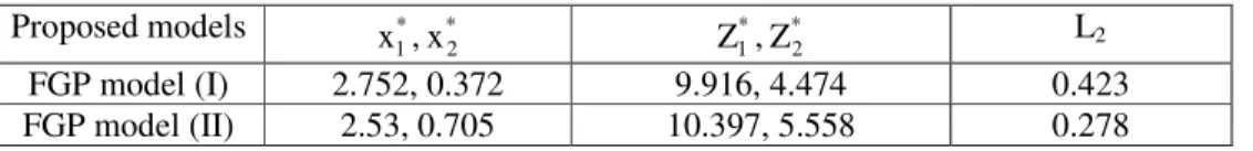
Table 1. Comparison of distances for the optimal solutions of the numerical Example 1 based on proposed two FGP models.

Proposed models * 1

x ,x *₂ Z ,₁* Z *₂ L2

FGP model (I) 2.752, 0.372 9.916, 4.474 0.423 FGP model (II) 2.53, 0.705 10.397, 5.558 0.278

Note 1: From table 1, we observe that the proposed FGP model (II) offers better optimal solution than the proposed FGP model (I) based on distance function L2 by considering same

preference bounds.

Example2. We consider the following QBLPP studied by Pal and Moitra [35]:

[ULDM]:

1

x

maxZ1 ( x ) = x1+2x - (x12 2-2)2

[LLDM]:

2

x

maxZ2 ( x ) = (x1 -2)2 +x 22

subject to x1 + x2 ≤ 6,

x1 +x2 ≥2,

-x1 +x2 ≤2,

-x1 +x2 ≥2,

x1, x2 ≥0.

We find the individual best solutionZ = 36 at (4, 2) and₁B Z = 16 at (2, 4) subject to the B₂ constraints for ULDM and LLDM respectively. Then the fuzzy goals appear in the form: Z1 ( x )

~

≥36 and Z2 ( x ) ~

≥16.

Payoff matrix = ₆ ₁₆ 8 36

Here, W 1

Z = 6 and Z = 8. 2W

The quadratic membership functions of both level DMs are constructed as:

µ1 ( x ) =

6 -36

6 -) x ( Z₁

=

30 ) 2 x ( x 2

x₁+ ₁2− ₂− 2

,

µ2 ( x ) =

8 -16

8 -) x (

Z2 ₌

8 8 x ) 2 x

( 22

2

1− + − _.

The membership function ₁(x) for ULDM is maximal at the point (4, 2) and the membership

(14)

54 functions are transformed into equivalent linear membership functions at the individual best (maximal) solution point by first order Taylor polynomial series as follows:

) x (

1

ξ = µ1 (4, 2) + (x1 - 4) (4,2)

x₁ 1

∂ ∂

+ (x2 - 2) (4,2)

x₂ 1

∂ ∂

,

) x (

2

ξ = µ2 (2, 4) + (x1 - 2) (2,,4)

x₁ 2

∂ ∂

+ (x2 - 4) (4,2).

x₂ 2

∂ ∂

Let 3 x1 5 and 2 x2 6 be the preference bounds provided by the respective level DMs.

Then the proposed FGP models can be written as:

= −

2

1 i di

subject to

1 + (x1 - 4) ×17/30 +d = 1, 1−

1 + (x2 - 4) ×1 +d = 1, −2

x1 + x2 ≤ 6,

x1 +x2 ≥2,

-x1 +x2 ≤2,

-x1 +x2 ≥2,

3 x1 5,

2 x2 6, 1 d 0≤ _i− ≤

(i = 1, 2), x1 0, x2 0.

Then, following the procedure, the proposed FGP model (I) gives the solution Z = 30, ₁* Z = 10 *₂

at x = 3, *₁ x = 3. The membership values are *₂ *₁= .467, *₂= .25

FGP model (II): minγ

subject to

1 + (x1 - 4) ×17/30 +d = 1, 1−

1 + (x2 - 4) ×1 +d = 1, −2

x1 + x2 ≤ 6,

x1 +x2 ≥2,

-x1 +x2 ≤2,

-x1 +x2 ≥2,

3 x1 5,

2 x2 6,

γ d , (i = 1, 2), −i

1 d

0≤ _i− ≤ (i = 1, 2). x1 0, x2 0.

The proposed FGP model (II) provides the same solution set Z = 30, 1* * 2

Z = 10 at x = 3, 1* * 2

x = 3.

The membership values are ₁*= .467, *₂= .25.

Pal and Moitra [35] obtained the same solution set. Using the same tolerance 1 for x1 and 2 for

x2, as considered in the proposed FGP models, Osman et al. [43] obtained leader’s individual

best solution (4, 2) which cannot be acceptable for the lower level decision maker.

(15)

55 [ULDM]:

1

x

min Z1 ( x ) = 3x + 412 2 2

x - 2x1- 2x2

[LLDM]:

2

x

min Z2 ( x ) = 5x +212 2 2

x - x1 - 2x2

subject to 2x1 + x2 2,

x1 + 3x2 7,

x1 0, x2 0.

The individual best (minimum) solution for ULDM and LLDM areZ = 0.158 at (0.789, 0.421) ₁B

andZ = 0.75 at (0.5, 1) respectively subject to the constraints. B₂ The fuzzy goals are as follows:

Z1 ( x ) ~

≤0.158 and Z2 ( x ) ~

≤0.75.

The payoff matrix is of the form

75 . 0 75 . 1

836 . 1 158 .

0 _{. Here,} W

1

Z = 1.75 and Z = 1.836. W₂

The quadratic membership functions for ULDM and LLDM are of the form:

1

ν ( x ) =

158 . 0 75 . 1

) x ( Z 75 .

1 1

− −

=

592 . 1

) x 2 x 2 x 4 (3x 75 .

1 1 2

2 2 2

1+ − −

−

and

2

ν ( x ) =

75 . 0 836 . 1

) x ( Z 836 .

1 ₂

− −

=

086 . 1

) x 2 x x 2 (5x 836 .

1 − ₁2+ 2₂− ₁− ₂

The quadratic membership function for ULDM is maximal at (0.789, 0.421) subject to the constraints and the quadratic membership function for LLDM is maximal at (0.5, 1) subject to the constraints. The quadratic membership functions ν₁( x ) and ν₂( x ) are transformed into equivalent linear membership functions at the individual maximal point as follows:

) x (

1

ξ = ν₁(0.789, 0.421) + (x1 – 0.789) (0.789,0.421)

x₁ν1

∂ ∂

+ (x2 -0.421) (0.789,0.421)

x₂ν1

∂ ∂

,

) x (

2

ξ = ν₂(0.5, 1) + (x1 -0.5) 1

x

∂ ∂

2

ν (0.5, 1) + (x2 -1) 2

x

∂ ∂

2

ν (0.5, 1)

Let 0.55 x1 1.5 and 0.5 x2 1.2 be the preference bounds provided by ULDM and LLDM

respectively.

The proposed FGP models for solving QBLPP can be formulated as:

= −

2

1 i di

subject to

1 + (x1 – 0.789) × (-1.717) + (x2 – 0.421) × (-0.859) +d = 1, 1−

1 + (x1 – 0.5) × (-3.683) + (x2 – 1) × (-1.842) +d = 1, −2

2x1 + x2 2,

x1 + 3x2 7,

0.55 x1 1.5,

0.5 x1 1.2, 1 d 0≤ _i− ≤

(i = 1, 2), x1 0, x2 0.

Solving the above FGP model (I), the solution set is obtained as Z = 0.188, *₁ Z = 1.562 at *₂ x = ₁*

0.75, x = 0.5. The resulting membership values are*₂ ξ*₁= 0.999,ξ*₂= 1.

(16)

56 subject to

1 + (x1 – 0.789) × (-1.717) + (x2 – 0.421) × (-0.859) +d = 1, 1−

1 + (x1 – 0.5) × (-3.683) + (x2 – 1) × (-1.842) +d = 1, −2

2x1 + x2 2,

x1 + 3x2 7,

0.55 x1 1.5,

0.5 x1 1.2,

γ d , (i = 1, 2), −_i

1 d 0≤ _i− ≤

(i = 1, 2). x1 0, x2 0.

By solving the FGP model (II) we get the same solution set Z = 0.188, *₁ Z = 1.562 at *₂ x = 0.75, ₁*

* 2

x = 0.5. The obtained membership values are ξ₁*= 0.999,ξ*₂= 1.

Note 2: From Example 3, we see that the proposed FGP model (I) and FGP model (II) offer the same solution set subject to the same preference bounds.

Note 3: We observe that the proposed two FGP models offer the same solution set or different solution set depending on the problem considered. Therefore, it is better to solve the problems by both the FGP models and use distance function L2 to identify the compromise optimal

solution.

Note 4:All solutions of the problem are obtained by Lingo software version 6.0.

9. C

ONCLUSIONS

In this paper, an alternative FGP approach has been studied for solving QBLPP. The proposed approach is easy to implement. Firstly, we transform QBLPP into a linear bi-level programming problem by using first order Taylor series approximation. Preference bounds provided by the upper and lower level DMs are considered for relaxation on decision. Then two FGP models are formulated in order to solve the problem by minimizing negative deviational variables. Here, we do not require positive deviational variables. We can apply the proposed concept to multi-level quadratic and multi-level quadratic fractional programming problem. The proposed concept can also be extended to solve QBLPP with fuzzy parameters.

The main drawback of the proposed approach is that it solves hypothetical problem. Here, for decision-making, degrees of membership functions of the objective goals are considered. However, But, degree of rejection should be simultaneously considered. In this sense, intuitionistic fuzzy sets due to Atanassov [48] and intuitionistic fuzzy goal programming technique due to Pramanik and Roy [49-51] could be applied to modeling QBLPP after using linearization technique.

We hope that the proposed FGP approach can contribute to future study in the field of practical hierarchical decision-making problems involving quadratic objectives especially in industrial, marketing, supply-chain management problems, etc.

Our future work will include the use of the concept presented in this paper to develop an algorithm for solving linear fractional / quadratic bi-level programming problem.

(17)

57

A

CKNOWLEDGEMENTS

The authors are very grateful to the anonymous referee for her helpful comments and constructive suggestions for improving the quality and presentation of the paper to its current standard. The authors are very grateful to Dr. B. C. Giri for his constant encouragements and constant support during the present study.

R

EFERENCES

[1] Candler, W. & Townsley, R., (1982) “A linear bilevel programming problem”, Computers & Operations Research, Vol. 9, No. 1, pp. 59-76.

[2] Fortuni-Amat, J. & McCarl, B., (1981) “A representation and economic interpretation of a two-level programming problem”, Journal of Operational Research Society, Vol. 32, No. 9, pp. 783-792. [3] Anandalingam, G., (1988) “A mathematical programming model of decentralized multi-level

systems”, Journal of the Operational Research Society, Vol. 39, No. 11, pp. 1021-1033.

[4] Lai, Y. J., (1996) “Hierarchical Optimization: A satisfactory solution”, Fuzzy Sets and Systems, Vol. 77, No. 13, pp. 321-335.

[5] Shih, H. S., Lai, Y. J. & Lee, E. S., (1996) “Fuzzy approach for multi-level programming problems”, Computers & Operations Research, Vol. 23, No.1, pp. 73-91.

[6] Shih, H. S. & Lee, E. S., (2000) “Compensatory fuzzy multiple level decision making” Fuzzy Sets and Systems, Vol. 114, No. 1, pp. 71-87.

[7] Sakawa, M., Nishizaki, I. & Uemura, Y., (1998) “Interactive fuzzy programming for multi-level linear problems”, Computers and Mathematics with Applications, Vol. 36, No. 2, pp. 71-86.

[8] Sinha, S., (2003) “Fuzzy programming approach to multi-level programming problems”, Fuzzy Sets and Systems, Vol. 136, No. 2, pp. 189-202.

[9] Sinha, S., (2003) “Fuzzy mathematical programming applied to multi-level programming problems”, Computers Operations Research, Vol. 30, No. 9, pp. 1259-1268.

[10] Arora, S. R., & Gupta, R., (2009) “Interactive fuzzy goal programming approach for bilevel programming problem”, European Journal of Operational Research, Vol. 194, No.2, pp. 368-376. [11] Vicente, L. N, & Calamai, P. H., (1994) “Bilevel and multilevel programming: a bibliography

review” Journal of Global Optimization, Vol. 5, No. 3, 291-306.

[12] Chen, Y., Florian, M., (1995) “The non-linear bilevel programming problem: formulations, regularity and optimality conditions” Optimization, Vol. 32, No. 3, 193-209.

[13] Edmunds, T. & Bard, J., (1991) “Algorithms for nonlinear bilevel mathematical problems”, IEEE Transactions Systems, Man, and Cybernetics, Vol. 21, No. 1, pp. 83-89.

[14] Savard, G. & Gauvin, J., (1994) “The steepest descent direction for the nonlinear bilevel programming problem”, Operations Research Letters, Vol. 15, No. 5, pp. 265-272.

[15] Abo-Sinna, M. A., (2001) “A bi-level non-linear multi-objective decision making under fuzziness” Journal of the Operational Research Society of India (OPSEARCH), Vol. 38, No. 5, pp. 484-495. [16] Malhotra, N. & Arora, S. R., (2000) “An algorithm to solve linear fractional bilevel programming

problem via goal programming”, Journal of Operational Society of India (OPSEARCH), Vol. 37, No.1, pp. 01-13.

[17] Sakawa, M. & Nishizaki, I., (2001) “Interactive fuzzy programming for two-level linear fractional programming problem”, Fuzzy Sets and Systems, Vol. 119, No. 1, pp. 31-40.

[18] Sakawa, M., Nishizaki, I., & Uemura, Y., (2000) “Interactive fuzzy programming for two-level linear fractional programming problems with fuzzy parameters” Fuzzy Sets and Systems, Vol. 115, No. 1, 93-103.

[19] Calvete, H. I. & Galé, C., (2004) “Solving linear fractional bilevel programs”, Operations Research Letters, Vol. 32, No. 2, pp. 143-151.

[20] Ahlatcioglu, M. & Tiryaki, F., (2007) “Interactive fuzzy programming for decentralized two-level linear fractional programming (DTLLFP) problems”, Omega, Vol.35, No. 4, pp. 432-450.

[21] Chakraborty, M., & Gupta, S., (2002) “Fuzzy mathematical programming for multi objective linear fractional programming problem” Fuzzy Sets and Systems, Vol. 125, No. 3, pp. 335-342.

[22] Charnes, A., & Cooper, W. W., (1962) “Programming with linear fractional functions” Naval Research Logistics Quarterly, Vol. 9, No.1, 181-186.

(18)

58 [24] Satty, T. L., (1980) The analytical hierarchy process, Plenum Press, New York.

[25] Júdice, J., & Faustino, A. M., (1994) “The linear-quadratic bilevel programming problem”, INFOR, Vol. 32, No. 2, pp. 87-98.

[26] Calvete, H. I. & Galé, C., (1998) “On the quasiconcave bilevel programming problem”, Journal of Optimization Theory and Applications, Vol. 98, No. 3, pp. 613-622.

[27] Vicente, L., Savard, G. & Júdice, J., (1994) “Descent approaches for quadratic bilevel programming”, Journal of Optimization Theory and Applications, Vol. 81, No. 2, pp. 379-399. [28] Wang, S., Wang, Q. & Romano-Rodriguez, S., (1994) “Optimality conditions and an algorithm for

linear-quadratic bilevel programs”, Optimization, Vol. 31, No.2, pp. 127-139.

[29] Thirwani, D. & Arora, S. R., (1998) “An algorithm for quadratic bilevel programming problem”, International Journal of Management and System, Vol. 14, No. 2, pp. 89-98.

[30] Calvete, H. I. & Galé, C., (2004) “Optimality conditions for the linear fractional/ Quadratic bilevel problem”, Monografias del Seminario Garcia de Geldeano, Vol. 31, pp. 285-294.

[31] Narang, R. & Arora, S. R., (2009) “Indefinite quadratic integer bilevel programming problem with bounded variable”, Journal of operational research society of India (OPSEARCH), Vol.46, No. 4, pp. 428-448.

[32] Etoa, J. B. E., (2011) “Solving quadratic convex bilevel programming problems using a smooth method”, Applied Mathematics and Computation, Vol. 217, No. 15, pp. 6680-6690.

[33] Li, H. C. & Wang, Y. P., (2011) “A genetic algorithm for solving linear-quadratic programming problems”, Advances Materials Research, Vol. 186, pp. 626-630.

[34] Mishra, S. & Ghosh, A., (2006) “Interactive fuzzy programming approach to bi-level quadratic fractional programming problems”, Annals of Operational Research, Vol. 143, No. 1, pp. 249-261. [35] Pal, B. B. & Moitra, B. N., (2003) “A fuzzy goal programming procedure for solving quadratic

bilevel programming problems”, International Journal of Intelligence Systems, Vol. 18, No. 5, pp. 529-540.

[36] Pramanik, S. & Dey, P. P., (2011) “Multi-objective quadratic programming problem: a priority based fuzzy goal programming”, International Journal of Computer Applications, Vol. 26, No. 10, pp. 30-35.

[37] Mohamed, R. H., (1997) “The relationship between goal programming and fuzzy programming problems” Fuzzy Sets and Systems, Vol. 89, No.2, pp. 215 −222.

[38] Moitra, B. N. & Pal, B. B., (2002) A fuzzy goal programming approach for solving bilevel programming problems, in: Pal, N. R. & Sugeno, M. (Eds.), AFSS 2002, INAI 2275, Springer-Verlag, Berlin, Heidelberg, 2002, pp.91-98.

[39] Pramanik, S. & Roy, T. K., (2007) “Fuzzy goal programming approach to multi-level programming problem” European Journal of Operational Research, Vol. 176, No.2, pp. 1151-1166.

[40] Baky, I. A., (2010) “Solving multi-level multi-objective linear programming problems through fuzzy goal programming approach”, Applied Mathematical Modelling, Vol. 34, No. 9, pp. 2377-2387. [41] Zeleny, M., (1982) Multiple criteria decision making, McGraw-Hill, New York.

[42] Ignizio, J. P., (1976) Goal programming and extensions, Lexington, MA: Lexington DC.

[43] Osman, M. S., Abo-Sinna, M. A.,, Amer, A. H., (2004) “A multi-level non-linear multi-objective decision-making under fuzziness” Applied Mathematics and Computation, Vol.153, No. 1, pp. 239-252.

[44] Sakawa, M., (2002) Multiple criteria optimization: state of art annotated bibliographic surveys, in:Ehrgott, M. & Gandibleux X. (Eds.), Kluwer Academic Publishers, Boston, Dordrecht, London, pp.171-226.

[45] Pramanik, S. & Dey, P. P., (2011) “Bi-level multi-objective programming problem with fuzzy parameters”, International Journal of Computer Applications, Vol. 30, No. 10, pp. 13-20.

[46] Pramanik, S. & Dey, P. P., (2011) “A priority based fuzzy goal programming to multi-objective linear fractional programming problem”, International Journal of Computer Applications, Vol. 30, No. 10, pp. 01-06.

[47] Yu, P. L., (1973) “A class of solution for group decision problems”, Management Science, Vol. 19, No. 8, pp.936-946.

[48] Atanassov, K., (1986) “Intuitionistic fuzzy sets”, Fuzzy Sets and Systems”, Vol. 20, No. 1, pp. 87 −

96.

(19)

59 [50] Pramanik, S. & Roy, T. K., (2007) “Intuitionistic fuzzy goal programming and its application in solving multi-objective transportation problem”, Tamsui Oxford Journal of Management Sciences, Vol. 22, No. 1, pp. 01-16.

[51] Pramanik, S. & Roy, T. K., (2007) “An intuitionistic fuzzy goal programming approach for a quality control problem: a case study”, Tamsui Oxford Journal of Management Sciences, Vol. 23, No. 3, pp. 01-18.

Authors

DR. SURAPATI PRAMANIK

He obtained Ph. D. in Mathematics from Bengal Engineering and Science University, Shibpur. He is the Assistant Professor of Mathematics in Nandalal Ghosh B.T. College. He is a senior life member of Operation Research Society of India, ISI (Kolkata) and Calcutta Mathematical Society. He received Golakpati Roy Memorial Award in 1988. His interest of research includes Fuzzy optimization, Grey system theory, Intuitionistic fuzzy decision making, Neutrosophic sets, and Math education. His paper together Partha Pratim Dey was awarded best paper in West Bengal State Science and Technology Congress (WBSSTC)-2011 in mathematics. His paper together with Manjira Saha was awarded best paper in WBSSTC-2010 in Social Sciences. His paper together with Sourendranath Chakrabarti and T. K. Roywas awarded best paper in WBSSTC-2008 in mathematics. He published research papers in International Journal of Computer Applications, European Journal of Operational Research, Journal of Transportation Systems Engineering and Information Technology, Tamsui Oxford Journal of Management Sciences, Notes on Intuitionistic Fuzzy Sets.

MR. PARTHA PRATIM DEY

Date of Birth: November 23, 1982. He passed B. Sc Honours and M. Sc in Mathematics in 2003 and 2005 respectively in the University of Kalyani. Currently, he is the assistant teacher of mathematics at Patipukur Pallisree Vidyapith, Patipukur, West Bengal. His fields of research interest include Fuzzy optimization, Decentralized bi-level decision making, Grey system theory, IFS sets, and Neutrosophic sets. His paper together with S. Pramanik was awarded best paper in West Bengal Science and technology Congress -2011 in Mathematics.