Public Debt Management, Monetary Policy and FinanciaI Institutions
Márcio G. P. Garcia
PUC-Rio
ThirdDraft
OS/28/2002
Abstract
1. Introduction ...•..•...•... 3
2. Decomposing the Public Debt Growth ...•. 3
3. Risk Measures for the Public Debt ...•... 5
3.1. Value-at-Risk (V@R) ... 7
3.2. Cash-Flow at Risk (CF@R) ... 11
3.3. V@R and CF@R Together ... 14
Rollover Risk ... 15
4.
4.1. 4.1.1. 4.1.2. 4.2. Mean-Variance with Rollover Risk ... 16An example with two assets ... 16
Rollover Risk and the Minimum Degree of Indexation ...•... 17
The Problem with Multiple Bonds ... 19
5. Monetary Policy and Public Debt Management ... 22
5.1. Monetary Policy Regimes and the Demand for Debt ... 22
5.2. Reserve Requirements ... 23
5.3. The FinanciaI Transactions Tax (CPMF) ... 24
5.4. Open Market Operations and the Provision of Liquidity to Banks ... 25
6. Conclusion and Policy Discussion ... 26
APPENDIX 1: Value-at-Risk Methodology ... 45
1.1- Nominal and Dollar Linked Bonds ... 45
1.1.1- Volatility Estimation ... 45
1.1.2 - Mapping: ... 45
1.1.3- Value-at-Risk: ... 46
1.2 - Inflation Linked Bonds ...•... 47
APPENDIX 2: Cash Flow at Risk Methodology ... 51
2.1 - Vector Autoregression estimation ...•...•... 51
1- Introduction
This paper analyzes several aspects pertaining to the management of the domestic public debt. The causes for the extremely large and fast growth of the domestic public debt during the seven-year period that President Cardoso are discussed in Section 2. Section 3 computes Value at Risk and Cash Flow at Risk measures for the domestic public debt. The rollover risk is introduced in a mean-variance framework in Section 4. Section 5 discusses a few issues pertaining to the overlap between debt management and monetary policy. Finally, Section 6 wraps up with policy discussion and policy recommendations.
2- Decomposing the Publíc Debt Growth
During the period 1995-2001, the Brazilian domestic public bonded debt more than quadrupled in real (percentage of GDP) terms. This Section decomposes the domes ti c federal bonded debt growth, searching for the macroeconomic causes of the very large growth that took place during the last seven-year period. We attempt to quantify the contraction and expansion sources of the federal bonded debt. The methodology used was developed in Bevilaqua and Garcia [2002], where it is thoroughly explained.
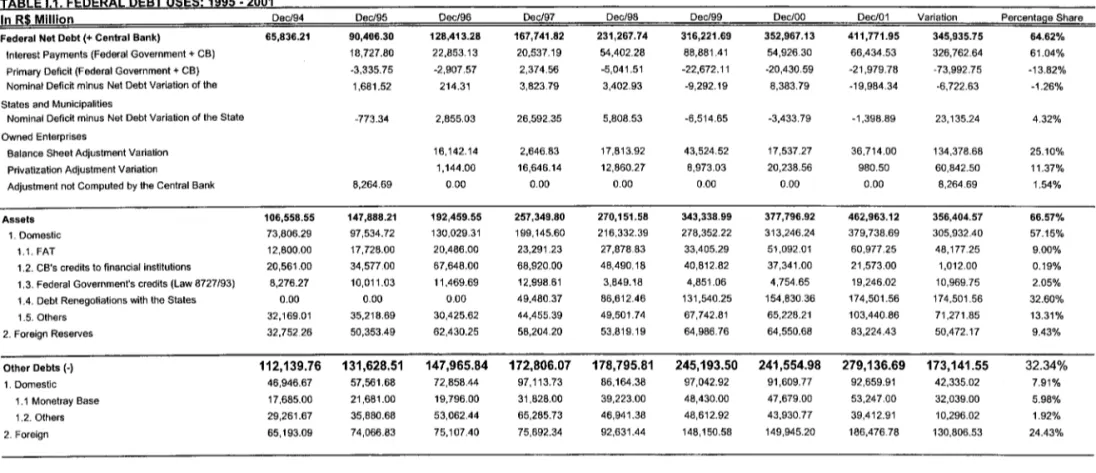
Table 1.1 displays the factors of expansion and contraction of the federal pub1ic debt (in nominal terrns). One must keep in mind that, since we are working with nominal values over a seven-year-period, the values presented on this table can be misleading.! The most important individual factor for debt growth was interest payments (61.04% of the total variation of R$535.343.38 ), followed by the accumulation of the state's debt (32.60%). This is a debt that several Brazilian state govemments owe to the federal govemment, the actual repayment of which will remain an open question in the next years. These two items alone add up to 93.64% ofthe total variation in the domestic federal bonded debt.
Table 1.2 displays the factors of expansion and contraction of the federal public debt (in real terrns, i.e., as percentage of GDP). The analysis in real terrns is the most relevant to the current economic situation The interest rate share increased even more in real terrns: interest payments (32.43% ofGDP) alone exceeded the full variation ofthe federal net debt (20.19% of GDP) and was almost equal to the total variation of the domestic federal bonded debt (36.13 % of GDP). If we compute the implicit real interest rate on the net debt, by dividing the nominal interest payments by the preceding net debt stock, we get the following figures:
Table 1.3
1995 1996 1997 1998 1999 2000 2001
l(t)/D(t-1 ) 28.45% 25.28% 15.99% 32.43% 38.43% 17.37% 18.82%
Y(t)/Y(t-1 ) 1.3401 1.1982 1.1091 1.0292 1.1311 1.0923 1.0841
(1 +1(t)/D(t-1 ))/(Y(t)/Y(t-1)) -4.22% 4.55% 4.58% 28.68% 22.38% 7.45% 9.60%
I We preferred to present first the nominal values so that the total value to be explained was equal to that
The line l(t)lD(t-l) contains the implicit net debt nominal interest rate, obtained through the division of the nominal interest payments in year t by the debt stock at the end of the previous year. Subtracting from this nominal interest rate the GDP growth rate
(Y(t)lY(t-1)), we obtain a measure of the excess of the nominal rate in relation to nominal GDP growth, which is the relevant variable to access how important the interest payments are in the growth of the debt to GDP ratio.2 Note that these implicit interest rates measure a lagged average of the current market rates. The lag length depends on the debt average remaining life, and its composition. For nominal debt, an interest rate increase would only show up in the figures above when the existing bonds at the time of the interest rate increase started to mature, and new ones were issued with a higher interest rate. However, if the debt is indexed to the interest rate or to other indices positively correlated with it, then the effect of the interest rate increase is either immediate or occurs sooner.
With this in mind, we may interpret the figures. The implicit excess interest rates were negative or low until 1997, and jumped upwards afier the start of the crises period in that year with the Asian crisis. 1998 and 1999 were years of extremely high interest rates, both because of the very high interest rates, and because of the devaluation, which impacted the US$-linked debt. In 2000, the implicit interest rate feU, and in 2001 it increased somewhat. Given that 2001 was also a crisis year, with successive interest rate increases in Brazil (the basic interest rate was raised from 15.25% in January to 19% in July), we may conc1ude that in the floating exchange rate regime, intemational crises no longer have such a heavy impact on the debt growth. Nevertheless, the figures for 2000 and 2001 are still cause for concem, since they are not as dose to zero as one would like.
The recognition of existing debts (skeletons) added up to 12.87% of GDP, with the bulk of it occurring during the 1999-2001 period. One would hope that most ofthe skeletons would already be out of the doset. However, bad surprises occur still quite ofien, and it would be an exceUent measure if the govemment could do an exhaustive job of opening every and each c10set to convey to the market what the bad shocks in the future will be. More important, it should make sure that the new skeletons are not currently being manufactured. The fiscal responsibility law is a major deterrent against the creation ofunfunded liabilities. However, the inventiveness of some public officials in bypassing the spirit of the law is always amazing, as it can be seen by the mushrooming of state and municipal pension plans. lt is quite likely that as these insufficiently funded pension plans start to have more retirees, a new skeleton will come out of the doset.
Privatizations revenues accounted only to less than half of the recognition of existing debts (6.09% of GDP). As far as privatizations are concemed, the performance of the period
2 The following equation represents the simplest debt dynamics, where D is the total debt, i is the interest rate
and X is public deficit: Dt = Dt_I(1+i,)+Xt
Dividing by the GDP (Y), we obtain:
セ@
=
D'_l . Y'-l (1 + i,) +セ@
=> d,=
d'_l' (1 + it) + x,, where Y, Y'-l Y, Y, (1 + g, )(1 + 7t,)d and x are the total debt and the public deficit over GDP, g is the growth rate ofreal GDP and 7t is the rate of inflation.
1999-2001 in comparison to the previous four-year period is not so good, reflecting the general slow-down in economic reforms that marked the second term of president Cardoso. The asset accumulation (16.24% of GDP) was almost completely accounted for by the increase in domestic assets (16.02%), many of which contain large credit risk. The state debts that were renegotiated constituted the bulk of the domestic assets (14.09% of GDP). Foreign Reserves were kept almost constant as % of GDP, thereby making the whole Asset Accumulation much less attractive as an indicator of solvency. This is why many analysts prefer to look at the gross debt, instead at the net debt as a measure of fiscal solvency. Other debts also remained fairly stable, while the foreign debt increased 2.12% of GDP. This increase reflects basically the change in the real exchange rate after the 1999 devaluation, and not an increase in the foreign debt in US dollars.
Therefore, the picture that emerges from the analysis of the very large increase in the domestic bonded debt is one where the privatization revenues were insufficient to counteract the appearance of lagged fiscal deficíts, in the form of the renegotiation of the state debts and other liabilíties (skeletons), as well as the large interest payments. Those figures highIíght the importance of avoiding the creation of new skeletons which may haunt the debt figures in the future, and of lowering the stíll very high interest rates.
1. Risk Measures for the Public Debt
Figure 1 displays the evolution of the federal domestic bonded debt structure since the start of the Real Plan, in July, 1994. Besides the very large and fast growth after mid-1995, whose determinants were analyzed in Section 2, the change in debt structure is àlso remarkable. Figure 2 displays the same data in a different graph format, so that the changes in composition are more cIearly visible.
The US$-linked bonds have grown during the whole period, both in real terms, as well as in % of the total domestic bonded debt. After an initial growth in the years following the beginning of the Real Plan, the share of pre-fixed (nominal) bonds have decreased dramatically, since the Russian crisis, being of small importance in the recent years, despite the iterated official intentions of issuing a larger share of nominal bonds.3 The place of the nominal bonds was taken by the zero-duration (SeIíc) bonds.4 These bonds constitute
3 See STN [2001], where the Treasury intended to have 22% of the total debt as nominal bonds until
December 2001. The document is available at
http://www.tesouro.fazenda.gov.br/hp/ downloads/plano _financiamento_di vida _8.4 .pdf
4 The bond indexed to the short-run interest rate (Selic) is a security sold at a discount which had its face value corrected daily by the average daily interest rates during its termo It is a floating interest rate, adapted to the high frequency required by the high inflation and daily indexation conditions prevalent when it was created (1985). It would be equivalent to a bond whose nominal value is accrued every day by the daily accrual of the Libor. This is the c10sest one can get to perfect indexation in fixed income markets. It
nowadays the majority of the domestic public bonded debt. Although the price-level-Iinked debt has increased its share in the total domestic bonded debt, its importance is still quite smal1. Other indexes account for some 5% ofthe debt.
As far as average remaining life is concemed, the debt has been lengthened quite substantially, as the nominal (short-term) bonds were replaced by the zero-duration bonds. However, average duration has not increased near1y quite as much. This discrepancy shows that refinancing (rollover) risk was given higher priority than market risk.
This Section aims at providing risk measures for the domestic debt. We do that by adapting the two best known risk measures used by financiaI institutions and non-financial firms, which are the Value at Risk and the Cash Flow at Risk. Refinancing (rollover) risk will be considered in the next Section.
Value at Risk (V@R)5 has become in recent years the standard tool for risk management among financiaI institutions. For corporate treasurers, V@R's offspring, Cash Flow at Risk (CF@R) is increasingly gaining acceptance.
V@R is defined as ... the worst expected loss over a given horizon under normal market conditions at a given conjidence levei (Jorion, 2001, p. xxii). The basic idea is to have one
number that summarizes the risk involved in the overall portfolio of a financiaI institution. There are several different methodologies to generate this number. The easiest one is the delta-normal. It assumes that the retums of the different assets and liabilities of a portfolio are multinormally distributed with zero mean. Since the portfolio's retum is a weighted sum of the multinormally distributed individual retums, it is also normally distributed. Therefore, if we take the difference between the portfolio value today, and the 5th percentile of its distribution tomorrow, we obtain the worst expected loss over a day under normal market conditions at a 95% confidence leveI, i.e., it is expected that only in 5% of the times, the loss will be over the V@R limit.
Non-financial enterprises are not so well characterized by their portfolios. To assess the risk, it is more important to quantify the impact of the risk factor in the profits and losses of the firms. For example, a large depreciation is bound to have a substantial negative effect in the future profits of an import firm, notwithstanding the fact that the immediate impact on its portfolio could be a positive one. The Cash Flow at Risk (CF@R) takes account of the impact on the firm's cash flow (Jorion, 2001, p. 366).
Here we propose to develop a V@R for the public debt and a CF@R the fiscal budget in Brazil. Together, these measures should provide a comprehensive risk assessment for the Brazilian public sector. The importance of these measures for policy purposes is likely to increase in the near future.
For example, the large nominal deficits registered in 1999 and 2001 were in great measure caused by the increase in value ofthe domestic debt due to the indexation c1auses present in
hand, monetary policy has a very limited wealth effect, as far as public is concemed, since rises in interest rates do not affect the value ofthe private financiai wealth in these fixed in come securities.
several bonds, both to the exchange rate and to the short ternl interest rate. Therefore, it is very important that the risk involved in the debt structure be adequately accessed, so that policy makers and the public can evaluate the true risklreward tradeoff involved in public debt management.
But fluctuations in risk factors as exchange and interest rates affect other components of the fiscal accounts besides the public debt. For example, the gains obtained by private agents that purchased exchange rate linked bonds in times of depreciation are partially taxed away through the income taxo This appears as an increase in tax revenues in times of depreciation. A V@R for the public debt would overestimate the negative impact of exchange rate depreciation on the fiscal accounts, because it would miss the increase in income taxo The CF@R would correct this flaw.
These risk measures would provi de a comprehensive risk assessment for the public sector accounts. This task has become even more important afier the second revision of the agreement with the IMF6 on 3/26/2002, when the Brazilian Central Bank was allowed to resume some trading in derivatives markets to rollover the existing exchange rate linked debt. Derivatives are off-balance-sheet items, usually with purchasing prices far below (zero for futures, forwards and swaps) the potentialloss that they may entail. Therefore, the only way one may appraise the potential loss involved in these items is through a risk measure as the V@R.
In Section 3.1 we spell out the methodology to construct the public debt V@R, and show its evolution since the devaluation in 1999. Section 3.2 contains the description of the CF@R methodology, as well as the relevant numbers. Finally, Section 3.3 puts the two methodologies together to construct a single measure for risk assessment.
1.1. Value-at-Risk (V@R)
1.1.1. Nominal Bonds
The methodology to compute the V@R for nominal bonds is quite standard. Jorion [2001] is a good reference, and Appendix 1 details the formulae used and data sources.
Basically what is done is the following. At any given date, we depart from the redemption schedule of the nominal bonds. Therefore, for each day, we have a list of future dates when coupons and/or the principaIs are repaid, with the present value (evaluated with the yield curve ofthat day) ofthose cash flows.
Given the history of interest rate variations, our goal is to compute the worst plausible outcome, defined as the 95th percentile ofthe distribution ofthe possible (stochastic) values of the total nominal debt in the following day. The standard V@R methodology assumes that the retums are multinornlally distributed with zero means and standard deviations and covariances to be estimated from the data. Therefore, the distribution of the overall
portfolio retum, by virtue of being a linear convex combination of the multinormal retums (weighted by the respective present values) is also normal, allowing us to compute the 95th percentile with the help of a standard normal distribution table.
Since the redemption schedule contains payments arbitrarily spread over future dates, we must choose a few dates (time vertices) to concentrate the payments, so that we can compute variances (and covariances) for those yields (interest rates). Having done that, for each day, we must also compute the variance covariance matrix for the time vertices. This is done through the exponentially weighted moving average (EWMA) model. [Jorion (2001), pages 193-196]
Figure 3 shows the evolution of the volatilities (standard-deviations) of the daily interest rates for the following time vertices: 5 days, 20 days, 40 days, 60 days, 80 days, 100 days, 150 days, 200 days, 250 days. To compute those volatilities, we were forced to use data from the derivatives markets at the BM&F-The Brazilian Commodities and Futures Exchange-, since there are no liquid secondary markets for govemment bonds in Brazil. Therefore, our calculations must be interpreted as an approximation that exc1udes liquidity risk. This is because lack of liquidity may cause the actual value loss when trying to sell a govemment security in any given day to be larger than the one implied by the movements in interest rates.
Figure 3 makes c1ear that the longer the period, the higher the volatility, so that the volatility yield curve would always be positively sloped. It also displays a pattem where spikes in all volatilities are followed by a decrease until another spike is reached. This pattem is due to the EWMA model.
For example, look at the beginning of the period, January 13, 1999, when the Real was floated. When that happened, interest rates for all vertices shot up, and that shows up in ·the increased volatility. The same data point of 1/13/99 ais o appears in the computation of the following day volatility, but with a lower weight (we used 0.95 as the decay factor). Therefore, until another shock makes interest rates increase a lot, the volatilities display a long-term mean reversion pattem. In that respect, it is interesting to note that the long-term averages have not yet come down afier the first quarter of last year, when the situation in Argentina worsened substantially.
portfolio, let alone a fixed income one denominated in the domestic currency. Other peaks occurred, as analyzed in the previous paragraphs, but the % V@R never went above half of the initial peak. The main reason for the decrease in the maximum V@R is that, in the floating exchange rate regime, the impact of crises (negative externaI shocks) are jointly shared by the interest and the exchange rate. For example, in March 2001, not only interest rates were increased, but also the exchange rate depreciated.
Notwithstanding the decrease in the interest volatility, it remains quite high, being a fundamental deterrent to the lengthening of the nominal debt. A back-of-the-envelope calculation help c1arify the point. In Brazil, the interest rate volatility remains high enough even the short maturities traded nowadays. Since the sensitivity of bond prices to the interest rate may be well approximated by the duration, which is similar to the maturity, we may conc1ude that if there were markets for longer term nominal bonds (say, five or ten years), the V@R would be much higher than variable income markets, defeating the very purpose of investing in fixed income securities. Therefore, it remains a tough, if not impossible, challenge to lengthen the debt with nominal bonds in the current Brazilian macroeconomic conditions.
1.1.2. Exchange-Rate-Linked Bonds
The computation of the V@R for US dollar-linked bonds is similar to the one for nominal bonds. Appendix 1 contains a detailed description of the calculation processo Here we shall emphasize the intuition. Suppose we were working with returns in US dollars. lf that were the case, the calculation would be the same as for the nominal bonds, explained before. However, we are working with returns in R$. Therefore, we should also consider the volatility of the exchange rate. Since V@R is about computing variances, we have to take account of the covariances between the returns of the exchange rate (the rate of depreciation) and the yields ofthe dollar-linked bonds for the several vertices (maturities). Figure 6 displays the volatility yield curve for the returns of the dollar-linked bonds. Since there are no liquid secondary markets for these bonds in Brazil, the volatilities are inferred from the prices of derivative securities at the BM&F-The Brazilian Commodities and Futures Exchange-, and, as before, must be interpreted as approximations that exc1ude the liquidity risk.
The extremely high volatilities at the beginning ofthe sample were caused by the very wild fluctuations of the US dollar during the first weeks of the depreciation, when it overshot from 1.21 R$ to 2.12 R$. In the derivatives market we used to get the data, the interest rate paid by a hypothetical dollar-linked-bond is determined by subtracting the forward premium (the expected depreciation plus the exchange rate risk) from the domestic interest rate. When the exchange rate is varying a lot (see Figure 7), that causes these implied rates to move a lot. 7 Figure 7 shows the volatílity of the spot US$IR$ daíly exchange rate.
lncidentally, these figures do not seem to corroborate any "fear offloating" in Brazil.
7 In spite of this plausible explanation, we are trying to get hold of an altemative dataset to check the
Figure 8 displays the V@R for the dollar-linked-bonds in % ofthe total dollar-linked debt.
It is substantially higher than the nominal bond V@R. This is a natural corollary ofthe fact that the risk here is measured against the basic interest rate in R$ (the Selic), and not against a retum is US$.
1.1.3. Zero-Duration Bonds
Zero-duration bonds, by definition, bear no market risk. This is because this bond is redeemed by the initial value capitalized by the accumulation of the daily basic interest rate (Selic). Since the present value of any asset is computed by discounting its redemption value by the accumulation of the daily Selic rates, the present value of this asset is the same, no matter what is the path of the Selic rate. Therefore, this bond bears no market risk. The reader familiar with the macroeconomic literature on optimal taxation may find quite strange to attribute zero risk to bonds that immediately start paying higher interest rates when there is an interest shock. After all, a positive interest shock coupled with a debt structure heavily weighted in zero-duration bonds is bound to generate a heavy burden to the fiscal budget, negatively impacting the necessary taxation. This only highlights the fact that the perception of risk to market players is different from the one relevant to the govemment. We can, however, adapt the threshold against which the V@R is measured. Govemment revenues growth would be an ideal but infeasible threshold. The same applies to nominal GDP growth. Inflation would probably be the best candidate, given the availability of price leveI data. However, retums on price-level-Iinked bonds are very hard to come by, as explained next.
1.1.4. Price-Level-Linked Bonds
To compute the risk of price-Ievel-linked bonds is a really difficult task. This is because on top of the inexistence of a liquid market for price-level-Iinked bonds, the derivatives market for the yields on those bonds is not only very illiquid, but is also very new. Therefore, we have very little data to work with. Appendix 1 describes all the hypotheses made to achieve proxies for the V@R ofthe price-level-Iinked bonds.
Figure 9 displays the first approximation (proxy 1) to the price-level-Iinked bonds V@R. It
considers only the inflation volatility, neglecting the possible yield variation. Given the low inflation volatility, proxy 1 leads to very low V@R measures.
Proxies 2, 3 and 4 try to take into account the volatility of the yields, which is much higher than inflation volatility. As a result, the V@R figures grow more than tenfold.
1.1.5. Total
V@R
To compute the total V@R we must basicalIy compute a variance ofthe overalI retum. For that, we would need alI the covariances between alI the risk factor considered previously, e.g., the covariance between the yield of a dolIar-linked bond of 250-day maturity and the yield of a nominal bond of 20-day maturity. The data required for some of those covariances are not available. Furthermore, by assuming extreme assumptions, i.e., correlations equal to + 1 and -1 between alI variables, we may get the lower and upper bounds of the total V@R.
Figure 12 displays the total V@R together with the debt figures (the zero-duration debt is exc1uded because it bears no market risk). Figure 13 displays the V@R as % of the debt. We see that after being very high immediately after the devaluation, the V@R decrease during 2000, and rose again in 2001, hovering below 1 % per day at that year-end.
Figure 14 displays the V@R as a % of GDP. We see the same pattem, with the V@R decreasing after the devaluation from 0.6% to 0.1 % of GDP by the end of 2000. During 2001, the V@R increases again, doubling by the third quarter, when it flattened and felI a little. Figure 15 displays the (daily) V@R as a % of (monthly) treasury revenues. The lines folIow the same pattem, but the magnitudes become more telIing. After reaching almost 30% of the revenues, the V@R is currently at the 10% of monthly revenues leveI. That means that the daily V@R is almost three times the daily treasury revenue, which is probably a very large magnitude.
As commented before, this measure is probably misleading as the relevant measure for the govemment. This is because when the interest rates rise, the interest payments related to the zero-duration bonds also rise, but the present value of these bonds do not, implying a zero market risk. The V@R is a good measure of the risk boni. by the private sector in holding the domestic public debt. Therefore, during 2001, not only the debt size grew substantialIy (see Figure 1), but the V@R as % ofthe total debt ais o doubled, thereby increasing a lot the risk bom the private sector in holding it. This is compatible with the increase in the implicit excess interest rates computed in Section 2.
1.2.
Cash-Flow at Risk (CF@R)The risk factors analyzed in the last subsections impact also the govemment's cash flows. Therefore, we borrow the concept of Cash Flow At Risk from the corporate literature to address this issue. The CF@R methodology (see Jorion, 2001, p. 366) requires the folIowing steps:
1) Compute the exposures of the cash flows to the risk factors; 2) Model the behavior of the risk factors; and
3) Simulate the risk factors and get the distribution of the resulting cash flows. The CF@R will be the difference between the 50th and the 5th percentile of that
In order to get item (1) above, we ran a V AR (Vector Auto-Regression) in proxies of the following five variables: real exchange rate, real interest rate, inflation, GDP growth, and primary surplus to GDP ratio. Non-stationary behavior was identified in a few ofthe series. This is probably due to the significant changes that fiscal and exchange rate policies underwent within the period. After the floating of the exchange rate in January, 1999, inflation shot up and has decreased afterwards, in line with a falling schedule of inflation targets. To account for the negative trend while inflation was converging to the new lower
leveI, we constructed a variable-the inflation gap-that measures the deviation of actual
inflation from the target, which is computed by interpolating the two targets for adjacent years. A similar thing was done with the fiscal surplus to GDP ratio. Since the last quarter of 1998, Brazil has an agreement with the IMF that promises to fulfill certain targets for the primary surplus, among other requirements. During 1999, the primary fiscal surplus to GDP ratio increased from zero to around the 3.5% leveI where it has been kept until today.
Also, to account for the trend, we constructed a variable-the fiscal gap-that measures
the deviation of actual surplus from the target, which is computed by interpolating the two targets for adjacent years. From the definitions used, the larger the inflation gap, the higher the inflation; and the larger the fiscal gap, the lower the primary surplus. In other words, positive values for the inflation and fiscal gaps mean that the targets are not being fulfilled. The resuIts are in Table 3.1. Appendix 2 contains the time-series variables charts.
The risk factors in this case are the contemporaneous shocks to the variables. We assume
they are muItinormally distributed with variances and covariances equal to those estimated through the V AR.
Finally, we use Monte Carlo simulation to get item (3) and compute the CF@R. The resuIts
are drawn in Figures 16 and 17.
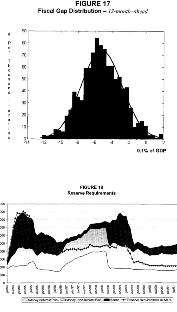
Figure 16 displays the histogram of the variable used to proxy for the primary surplus-the fiscal gap. As explained before, when the fiscal gap is negative, the primary surplus target (currentlyat 3.5% of GDP) is surpassed. We simulated 1,000 one-month-ahead scenarios.
The little dots represent the 5th and the 95th percentiles. We are interested in the latter, since
higher resuIts mean lower primary surpluses. We see that the primary surplus target is not at all in jeopardy when one considers the shocks to the exchange rate, the interest rate, the GDP growth, and inflation. On the contrary, those shocks tend to increase the primary surplus (the starting value was zero).
If we keep shockíng the system for 12 months, we get a slightly different result. Figure 17
shows this case. The distribution of the fiscal gap is more spread, as expected, but the 95th
Table 3.1
Vector Auto-Regression Estimation
Sample: 1999:052002:01 Included observations: 33
Standard errors & t-statistics in l2arentheses
liRER Real Inflation Output Fiscal Gap Interest Gap Growth
Rate
liRER(-1) 0.433689 0.152833 0.028182 -0.262320 -0.039040
(0.17612) (0.14628) (0.02919) (0.09512) (0.00962) (2.46246) (1.04479) (0.96540) (-2.75767) (-4.05936)
Reallnterest Rate (-1) -0.109766 0.710234 0.008366 -0.062864 -0.010766
(0.17517) (0.14549) (0.02903) (0.09461) (0.00957) (-0.62663) (4.88164) (0.28815) (-0.66445) (-1.12557)
Inflation Gap(-1) -0.399522 0.528311 0.959459 -0.582926 -0.085243
(0.66246) (0.55022) (0.10980) (0.35780) (0.03617) (-0.60309) (0.96017) (8.73800) (-1.62919) (-2.35644)
Output Growth( -1) -0.140137 0.027067 -0.014530 -0.559655 -0.020766
(0.28852) (0.23964) (0.04782) (0.15583) (0.01575) (-0.48571 ) (0.11295) (-0.30384) (-3.59140) (-1.31804)
Fiscal Gap( -1) 3.699937 3.047467 -0.619063 -2.087710 0.287218
(2.56685) (2.13196) (0.42545) (1.38638) (0.14017) (1.44143) (1.42942) (-1.45506) (-1.50588) (2.04914)
C 0.030247 0.030481 -0.001198 0.011345 -0.000124
(0.02199) (0.01827) (0.00365) (0.01188) (0.00120) p.37525} p.66861 } {-0.32867} {0.95505} {-0.10354}
R-squared 0.322041 0.568699 0.877845 0.404351 0.637631
Adj. R-squared 0.196493 0.488829 0.855224 0.294045 0.570525
Sum sq. resids 0.024557 0.016941 0.000675 0.007164 7.32E-05
S.E. equation 0.030158 0.025049 0.004999 0.016289 0.001647
F-statistic 2.565080 7.120266 38.80624 3.665736 9.501918
Log likelihood 72.02900 78.15509 131.3391 92.35659 167.9802
AkaikeAIC -4.001758 -4.373035 -7.596311 -5.233732 -9.816979
Schwarz SC -3.729665 -4.100943 -7.324218 -4.961640 -9.544887
Mean dependent 0.007124 0.100634 0.008873 0.003310 -0.002881
S.D. del2endent 0.033644 0.035035 0.013137 0.019386 0.002513
Determinant Residual Covariance 1.79E-21
Log Likelihood 554.1592
Akaike Information Criteria -31.76722
1.3. V@R and CF@R Together
We may now consider the two measures together, the V@R and the CF@R. As explained in Section 2.2, considering the impact of the shocks to the exchange rate, the interest rate, the GDP growth, and inflation tends to improve the primary surplus. Therefore, it would tend to lower the budgetary impact of negative shocks that increase the debt. In other words, the primary surplus tend to act as a shock absorber (albeit a weak one) to the increase in the debt stemming from shocks to the exchange rate, the interest rate, the GDP growth, and inflation. This may be explained, for example, by of the extra income tax that the recipients of the higher interest rates that are paid on govemment debt when the exchange rate depreciates or the basic interest rate (Selic) is raised must pay. However, to determine exactly where this increase in the primary surplus comes from it would be required a study of the fiscal accounts, which is beyond the scope of this paper.
2. Rollover Risk
The policymaker's decision of what kind of debt to fioat (denomination, indexation, and maturity) may be described as follows. Given the govemment's objective function, the debt manager has to decide which bonds and in what quantities to fioat. The debt manager maximizes the govemment's objective function based on the history ofthe rates ofretum of the several bonds and their statistical properties (expected retum, variance, etc.).8
This maximization probIem may be interpreted as the symmetric of the portfolio allocation decision, in which the investor decides his portfolio composition by maximizing his utility function defined over wealth or consumption. Several models of portfolio allocation are availabIe, the most famous being the Mean-Variance anaIysis ofMarkowitz [1952].
OnIy very strict hypotheses may justify that expected utiIity be defined exclusiveIy over expected retums and variances for arbitrary distributions of retums and utiIity functions.9 NevertheIess, Mean-Variance (MV) anaIysis, since its deveIopment by Markowitz fifty years ago, has become by far the most wideIy known principIe of portfolio allocation. Here we adapt the MV anaIysis for the pubIic debt manager probIem. Two features of this adaptation are worth of noting. First, the expected retum for the bond holder is converted in expected cost for the debt manager. Therefore, the debt manager disIikes higher expected returno Second, the safest asset for the bondholder (let's say, the asset perfect1y indexed to consumption) is the riskiest for the govemment. What happens here is that the risk is shifted from one side to the other.
Another important risk source that is considered by the debt manager is the rollover risk. Several studies emphasize the importance of not allowing Iarge portions of the pubIic debt to mature at the same time, since that may expose the govemment to pay abnormally high rates of retum to roll the debt over, or even be forced to monetize the domestic debt or default on the foreign debt. Therefore, Iengthening the debt maturity is also an objective of the debt manager in order to avoid the rollover risk. We posit a very simpIe way to model this rollover risk that is compatible with MV anaIysis, so that we can still reIy on its well-known mathematics to deveIop the policy impIications.
8 Missale [1999] deseribes several approaehes to the debt management problem.
9 As shown by Huang and Litzenberger [1988], pp. 60-62, there are basieally two ways to justify the
2. 1.
Mean- Variance with Rol/over Risk
The goal is to adapt the widely used MV analysis of Markowitz [1952] to the debt management problem, also incorporating the rollover risk. In order to do that, we will resort to an example with two assets, and then will generalize the problem to three or more kinds ofbonds.
2. 1. 1. An exam pie with two assets
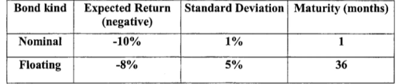
Suppose there are only two bonds. The nominal bond is a regular zero-coupon bond. Its retum in domestic currency, R$, is known in advance. The other kind of bond is the floating bond, whose retum varies with the interest rate. For the sake of this example, we assume the following parameter values:
TABLE 4.1: PARAMETERS VALUES
Bond kind Expected Return Standard Deviation Maturity (months) (negative)
Nominal -10% 1% 1
Floating -8% 5%
36
We also assume that the rates of retum on both assets have zero correlation. Note that the govemments dislikes expected return, therefore, ceteris paribus, the debt manager would
like to maximize the negative of the expected return, which corresponds to cost minimization. This, of course, is the symmetric of the standard investor attitude, which seeks to maximize the expected returno
Note also that the floating bond vo1atility (standard deviation) is higher that the nominal bond's, which may sound counterintuitive despite the difference in maturities. The explanation, besides the longer maturity of the floating bond, is that for the govemment what counts is the volatility ofthe deflated future value at the maturity, not the volatility of the marked-to-market price (the volatility of the present discounted value of the bond). For example, take a floating bond perfectly indexed to the interest rate, as the zero-duration bond. When the interest rate rises, the bond's present discounted value does not change. However, the amount in R$ to be disbursed at maturity increases substantially, and, if inflation remains stable, so does the real value of the disbursement. This is assumed to be the volatility (market risk) that matters for the government. 10
10 We could altematively, adapt the model to other risk factors by measuring the volatility ofthe ratio ofthe
Again, as in the case of expected retum, the govemment objective function is the opposite of the investor. However, since variance is independent of the deviation from the mean sign, it is nonsense to change the sign, as we did with the expected retum. The adaptation that makes sense is to realize that an indexed bond, i.e., a bond whose present discounted value varies very little, thereby being a safe investment for the holder, is very risky for the issuer, i.e., the govemment. That is what is accomplished by measuring the standard deviation in the way sketched above.
Therefore, one could approximate the standard deviation of the nominal bond by the standard deviation of monthly inflation, and the standard deviation of the floating bond by the standard deviation of the three-year real interest rate. The numbers in the example are merely for illustrative purposes.
With these adaptations, the MV diagram for the govemment is displayed in Chart 1. The govemments' indifference curves should be positively sloped and convex, with the govemment's objective function increasing as the curves move toward the northwest. Therefore, the efficient set is formed by alI combinations (portfolios) of bonds that are above the minimum-variance portfo1io, as it is the case in standard MV analysis.
2.1.2.
Rollover Risk and the Minimum Degree of Indexation
So far the adaptations made in MV analysis are fairly mild. Now, we introduce a new source of risk, the refinancing (rolIover) risk. It is the risk that the debt manager may be placed in a comer when she needs to rolIover a large portion of the debt, thereby having to offer extremely high yields (low bond prices). IdealIy, such risk should show up in the rate of retum distributions, i.e., the probability distribution of bond retums should incorporate these "comer" events. Here, we take a short-cut, that may correspond to a distribution which incorporates these comer events.
The rolIover risk depends positively on how welI spread through time the bonds' maturities are. The more spread apart they are, the lower the risk that the debt manager be placed in a comer. A proxy for how well spread the bonds' maturities are is the average maturity ofthe bond. The issuance of very short-maturity bonds tends to concentrate the bonds' redemption, e.g., if only one-month bills were issued, the whole public debt would eventually mature within the following month.
Therefore, one possibility for modeling the rates of retum distribution of public bonds is that its variance varies according to the average maturity of the debt stock. The higher the debt average maturity, the lower the rollover risk, and the lower the variance ofthe bonds' retums at the placement auctions. We could calI this model HCDM, for Heteroskedasticity Conditional on Debt Maturity.
- Expected Cost = -
[aE(RJ+
(1-
a )E(RF)]
(1)Modified Variance=
{(a
2o-
2{RJ+{I-aY
0-2(RF)
+
2pa{RJo-{RF )a{l-a)]
where,
RN
=
nominal bond return RF = floating bond return+
17[(MI
RN
+
{1-a)MRF -MRJ2]}
(2)a
=
portfolio weight on the nominal bond (l-a) = portfolio weight on the floating bond MRN = nominal bond maturityMRF
=
floating bond maturity 11=
roIlover risk weight E(.)=
return's expected value <1>(.)=
retum's standard deviationセ@
=
returns' correlation coefficientThe parameter 11 is the weight that incorporates to the variance the effect of the roIlover risk. Chart 2 shows how the incorporation of rollover risk affects the MV ana1ysis. The curve labeled 11=0 is the one of Chart 1. As 11 increases, the risk, as measured by the modified standard deviation, also increases for all portfolios but the one with 100% allocated in the longest maturity bond. For 11=0.000002, the risk of the 100% short-term portfolio equals the risk of 100% long-term portfolio. For 11>0.000002, the risk ofthe 100% short-term portfolio exceeds the risk of 100% long-term portfolio. As 11 keeps increasing, the rollover risk becomes completely dominant, as shown in Chart 3.
Chart 4 displays the same data in the space Maturity vs. Standard Deviation. Since the portfolio maturity is also a linear convex combination of the two bonds' maturities, as it is the case ofthe expected retums, Chart 4 has the same shape as Chart 2.
exchange rate overshooting that followed-, the risk tumed into reality, and the debt increased much more than it would have increased were it composed in its majority by nominal (nominal) bonds.
TABLE 4.2: MINIMUM INDEXATION AND MINIMUM MATURITY
11 Minimum Portfolio Weight On Minimum Maturity
Floating Bonds (months)
0.000000000 4% 2.4
0.000001000 35% 13.3
0.000002000 50% 18.5
0.000005000 72% 26.2
0.000009000 82% 29.7
0.000010000 83% 30.1
0.000100000 98% 35.3
0.000406041 100% 36
What happened in Brazil may be modeled by an increase in the parameter 11. The debt structures that leave the efficient set as 11 increases are the ones with more nominal and less floating bonds. As the rollover risk becomes more important, the "optimal" debt structure tends to display a longer maturity, precisely to diffuse the rollover risk. Table 2 shows this characteristic of the model. With 11 sufficiently high (equal to 0.000406041 and above), only 100% floating bonds portfolios are acceptable.
2.2.
The Problem with Multiple Bonds
In the two-bond case, we saw that the "modified" variance was:
_ {[a
2O'
2(R
N )
+ (1- af
0'2(R
F )+ 2pO'(R
N)cr(R
F)a(l- a)]+}_
- +YJ[(a
2(MRN- MRFf)]
Tj[wjM j +W2M2 +(l-wj -w2)M 3 -M3]2 =
=Tj[wjM j +W2 M2 -(Wj +w2)M3
J2
==Tj[wj(M j -M 3)+W2(M2 -M3
W
=[ l[
(Mj - M3)2=Tj Wj W2
(M j -M3)(M 2 -MJ (4)
Therefore, it is easy to see that, in order to compute the "modified" variance, all one needs to do is:
1 - reorder the n bond kinds, so that the last one is the longest;
2 - take the original variance-covariance matrix, O (n x n), and consider the
principal minor «n-J) x (n-1» formed by elimination ofthe last row and column;
3 - to each cell (Oij) of the principal minor add [T](Mi - Mn) (Mj - Mn)], i < n ,j > n ;
4 - put back the nth row and nth column that had been previously eliminated to get
the modified variance-covariance matrix, OMOD ;
5 - the modified variance is simply
Modified Variance = I' OMOD 1 where,
1 = vector (n x 1) ofportfolio weights;
OMOD
=
modified variance-covariance matrix.Now, all we need to do is to prove that the modified variance-covariance matrix is positive definite. This is easily accomplished by noting that the modified variance is obtained by adding to the original variance (itself a quadratic form with a positive definite matrix) a quadratic term that is greater than zero whenever all bonds are not of the same (i.e., the longest) maturity. Therefore, the modified variance-covariance matrix must also be positive definite.
3. Monetary Policy and Public Debt Management
In this Section we analyze a few issues pertaining to the overlapping of monetary policy and public debt management. In every country both policies are related. However, this is more so in Brazil, because of the domestic currency substitution process that characterized the megainflation ofthe 80s and the first half ofthe 90s.
Regular currency substitution was avoided through the provision of regular bank deposits that were protected from inflation. Those deposits, which were considered as money and had daily liquidity, were backed by govemment debt. Monetary policy became completely passive because it could not jeopardize the domestic currency substitution mechanism by raising interest rates. Although this state of affairs has changed substantially after the Real Plan, a few characteristics oftoday's monetary operation mechanism are inherited from that period.
3.1. Monetary Policy Regimes and the Demand for Debt
As analyzed elsewhere, II Brazil was able to retain a fairly stable demand for its national currency during the megainflation years through the provision of (domes ti c) currency substitutes protected from inflation erosion. In those years, the Central Bank monetary policy was restricted to provide a positive and not very volatile real interest rate. FinanciaI intermediaries would carry govemment bonds in their balance sheets and provide money market accounts that were widely perceived as being protected from inflation, unlike the regular currency. Were the Central Bank to raise interest rate to deter the inflation, it would impinge large losses to the financiaI intermediaries, thereby jeopardizing their ability to provide inflation protected domestic currency substitutes. Not surprisingly, the monetary policy was completely accomodative as inflation drifted upwards until it was successfully stoped by the Real Plan ofJuly, 1994.
Since monetary policy was de facto precluded from exerting its main goal, i.e., to fight
inflation through the interest rate management, debt managers engineered the zero-duration bonds (see Section 3) to save the volatility premium that appeared in the bonds' auctions. In other words, financiaI institutions would purchase short-term nominal debt with a sizeable discount because of the interest rate risk. Note that the interest rate risk during megainflation is essentially driven by the jumps in inflation expectations, which are much higher than the changes in the real interest rate. With zero-duration bonds the interest rate risk was eliminated, and the govemment could sell bonds at a higher price.
However, with the zero-duration bonds, monetary policy becomes completely devoided of any wealth effect. Interest rates may rise or fall, and the present value of the zero-duration debt will remain constant. Of course, this (tautological) statement has to taken with a grain of salt. After all, if the domestic interest rate were to fall too much, violating the bounds
imposed by interest parity conditions, a capital outflow would result, since the domestic interest rate would no longer serve as tmsted benchmark.
After the Real Plan, financiaI intermediaries remained addicted to govemment bonds whose prices have very low of zero volatility. Until 1997 (see Figure 1), the lenghtening through nominal debt procedeed, only to be interrupted by the Asian crisis. Increases of more than 2000 basis points in the basic interest rate happened a few times until 1999, alI but killing the prospects of a demand for long nominal bonds. Although in the current floating rate regime the exchange rate also serves as a shock absorber, thereby decreasing the interest rate volatility, the lenghtening of the nominal debt has yet to reach the two-year maturity that was being auctioned just before the Asian crisis.
FinanciaI intermediaries used to look for the zero duration bonds that have no market risk so that they could provi de money market funds whose yields track the basic interest rate benchmark (the Selic rate). Quite recently, however, given the introduction of stricter mIes forcing the fund industry to observe mark-to-market practices, as welI as the uncertainty pertaining to the electoral process (will the next president tamper with the public debt?), even the zero-duration debt has been trading with a sizeable discount (sometimes above 100 basis points). This discount reflects jointly liquidity and credit risks, and has been causing losses for many market funds, forcing them to offer their c1ients negative yields. Negative yields were considered an anathema in the fund industry, and it is still unc1ear what this new state of affairs-where the agents no longer have (at least the feeling of) a complete safe haven from liquidity and credit risks-will entail.
3.2.
Reserve RequirementsReserve requirements were always very large during the megainflation years, and are still quite high. Figure 18 shows the reserve requirements evolution, as welI the ratio of total reserve requirements to M4 (RHS scale). When the Real Plan started, in July 1994, the reserve requirements were raised because of fears that the increase in money demand could be confounded with inflationary money printing, and to deter excess credit expansion that could jeopardize the initial phase of the plano As the plan became more and more successful, the reserve requirements were further raised to prevent excessive growth of the aggregate demando Even a reserve requirement of 15% on bank loans was imposed.12 High reserve requirements serve not only as a deterrence against excessive credit expansion-always a danger in a country with such a low total credit to GDP ratio as Brazil (less than 30%)--, but also to a very convenient and cheap way of rolling over the debt (part of the reserve requirements are to deposited in govemment bonds). Since inflation targeting was adopted as the monetary policy framework in May 1999, the Central Bank has tried to lower the reserve requirements. However, last year, to prec1ude banks from speculating in the exchange rate markets (buying dolIars), the Central Bank decided to raise
reserve requirements on time-deposits. Therefore, this tooI seems to still be used for many different purposes.
Recently, with the introduction ofthe reaI-time-gross-settlement payment system, the Iarge reserve requirements have proven to be very useful. This is because the Central Bank allows banks to use their reserve requirements during the day to settle transactions, thereby providing enough extra Iiquidity to meet the extra Iiquidity needs that arose from the passage of a net-deferrement system to a reaI-time-gross-settlement payment system. In summary, it seems that the Iarge reserve requirements that were inherited from the megainflation years will prove to be very difficult to be reduced to the very Iow leveIs currently in place in most OECD countries, since they have a very high "opportunistic" value as a tooI to obtain severaI different objectives.
3.3. The Financiai Transactions Tax (CPMF)
Since it has been reinstated in 1997, the tax on financiaI transactions (CPMF) has become a major revenue source for the budget, as shown in by the numbers below. Current1y, it aIso serves as a means to find tax evaders, by picking up those with little (reported) income and high payments of financiaI taxo Recently, Congress has exempted stock market operations from the tax, a measure Iong due. Banks are aIso exempted in their activities. The financiaI tax is, thus, much more important for the fiscal policy than for monetary policy or for debt management.
The financiaI tax acts as a deterrent to the increase of Iiquidity of public debt secondary markets. Since only financiaI institutions are exempted from this tax, all other possible players in the secondary debt market have to bear this extra cost. Therefore, short-term operations involving debt (as repos) become very expensive. The current preferred tax vehicle seems to be the "exclusive fund".
Table 5.1
Constant R$ Million (Dec/2001 \
CPMF Revenue Total Treasury Revenue CPMF's share of the Total
1997 8,842.45 139,838.13 6.32%
1998 10,096.10 171,230.49 5.90%
1999 9,299.88 249,866.88 3.72%
2000 16,121.53 261,813.03 6.16%
3.4. Open Market Operations and the Provision of Liquidity to Banks
Open market operations represent the main operating channel linking monetary policy to debt management policy. Given the institutional idiosyncrasy that tax and loans accounts must be in the Central Bank (this is a constitutional c1ause), the Central Bank has a lot of work deriving from the administration of the Treasury's accounts. In days when the civil servants get paid, the Treasury first transfers the funds to the banks, and the Central Bank must conduct contractionary open market operations to mop up the banks' excess liquidity until actual payments are made. Conversely, in days were the banks are due to transfer to the Treasury the taxes they have collected, the Central Bank must conduct expansionary open market operations to replenish the banks with reserves. If it did not act in this way, the basic interest rate would fluctuate wildly. This is a very interesting feature of the Brazilian monetary system: because the interest rate would fluctuate too much if the Central Bank did not intervene often, it ends up intervening so strongly as to shut off completely any intra-day variability in the basic interest rate.
4.
Conclusion and Policy Discussion
The management of the domestic public debt is perhaps the single most important issue currently in the economic policy agenda, as we11 as in the presidential candidate's economic programs. This is due to its large size (above 50% of GDP), as we11 as the extremely high and counter-cyclical interest rates, which inflicts a higher to11 on the budget precisely when the economy is weak. Both factors jointly threaten to put the debt in an unsustainable path. Simulations13 show that under reasonable assumptions, the tough fiscal stance, currently delivering a primary surplus of3.5% ofGDP, must be maintained in the next years in order to keep the debt to GDP ratio from growing further.
Here, we analyze several aspects pertaining to the management of the debt. Section 2 studies the causes for the extremely large and fast growth of the domestic public debt during the seven-year period that President Cardoso has been in power (until the end of 2001). The data show that interest payments were by far the largest culprit for the debt growth. Other components, as the accumulation of assets and hidden liabilities were also important. Furthermore, given that many of the assets, especially the state debt, are of doubtful value, the picture displayed by the net debt figures may underestimate the true situation.
The macroeconomic summary behind the data is the following. In the first years of the Real, the fiscal stance was quite lax. Given the weak fiscal stance, monetary policy was then used to prevent the excessive growth of aggregate demand that would threaten the main achievement of the plan, the low inflation. During most of this period, foreign capital was flowing in, forcing the government to impose controls in capital inflows to prevent the appreciation ofthe real. 14
This state of affairs changed after the Asian crisis. Then, interest rates had to be raised to avoid capital outflows, which would threaten the managed exchange rate, and, therefore, also threaten inflation stability. This situation became prevalent until the beginning of 1999, when the real was floated, and the new monetary policy regime was created according to the new world paradigm of inflation targeting. Since 1998.3, a new, and much tougher, fiscal stance had been put in place, with ambitious targets for primary surpluses, which the Brazilian government has been fulfilling until present. However, the composition of the debt, roughly half indexed to the short term interest rate and a fourth indexed to the exchange rate, maintained the debt growth rate at high leveIs in face of externaI shocks that caused real depreciation and required higher interest rates to ensure that the inflation targets were not abandoned.
Section 3 implements risk measures for the domestic public debt. Value at Risk (V@R) measures are computed for the different debt components, as well as for the aggregate. Given the lack of liquidity, which prevented us from having the necessary bonds' prices, a
13 Several investment banks (JP Morgan, Deutsch Bank, etc) regularly produce debt sustainability simulations. See also Bevilaqua and Garcia [2002].
few heroic assumptions had to be made to allow the computation of the V@R. The results show that the risk bome by the govemment shot upwards during the floating of the currency, when volatility grew a lot. After that, it decreased steadily until the beginning of 2001, when several shocks started hitting the economy (the recession in the US, the contagion from Argentina, the energy crisis and political problems among the govemment allies in Congress). AlI these increased volatility and risk, as measured through theV@R. The V@R measures the worst plausible loss of a portfolio present value. Present values in Brazilian domestic currency are usualIy computed by discounting the future values by the domestic interest rate (Selic). Therefore, the zero-duration bonds, whose stock amounts to more than 50% of the domestic public debt, bear no risk. This causes the V@R to underestimate the budgetary risk that is relevant for govemment decisions. After an, when interest rates are raised, the present value of the zero-duration debt does not change, while the real value of interest payments do increase, be they deflated by the price leveI, or computed as % of GDP. Even with this bias toward underestimation, when computed as a
% of Treasury's revenues, the risk proves to be very high. Each day, the worst plausible loss (increase) in the value of the domestic debt corresponds roughly to three times the daily Treasury' s revenue.
In order to incorporate the impact of the shocks to the budget, the concept of cash flow at risk (CF@R) was adapted to the govemment budget. The impacts of several variables as the interest rate, the exchange rate, the GDP growth rate and inflation on the primary balance were computed through a vector auto-regression (V AR). The results show that shocks to those variables have a positive impact on the primary surplus, although the magnitude is smalI when compared to the increase in the debt value that the same shocks would cause.
Section 4 considers the rollover risk in the context of the widely known mean-variance analysis. It is shown that the decisions regarding the debt composition that were taken in May, 1998 could be interpreted as shocks that tilted the govemment's trade-off between market risk and rolIover risk. Further work is necessary to implement the model with parameters that accurately represent the problem faced by the Brazilian public debt manager.
This habit ofhaving daily liquidity and high real interest rates did not subside with inflation stability. Money market funds are stilI obliged to offer positive real returns with daily liquidity, ar so they feeI. The problems that are currently surfacing in the domestic debt markets, as the presidential elections polIs bring fears that a (partial) default may be favored by the next president, reflect to a great extent this habit that Brazilians grew accustomed to having. As even zero-duration bonds, which are free from interest rate (market) risk, begin to be traded at large discounts reflecting credit and liquidity risks, money market funds are no longer alIowed to pretend that they are able to offer daily liquidity with no risk. This is bound to have an impact on the demand for domestic debt, although it is not currently clear to which extent.
The many different roles of reserve requirements were also reviewed. The general conclusion is that the high reserve requirements very often help the monetary authority to achieve certain ancillary goals that have nothing to do what reserve requirements are for. For example, reserve requirements were used as a means to control credit expansion, speculation in the foreign exchange markets, and to provide intra-day limits for banks to operate in the newly released real-time-gross-settlement payment system. For that option value, it is likely that reserve requirements will be kept for much longer at the current very high leveIs.
The financiaI transaction tax detrimental role in preventing greater liquidity in the public debt secondary market is also mentioned. FinalIy, the management of bank reserves through open market operations is studied. The Brazilian Constitution mandates that alI govemment bank accounts be kept at the Central Bank. This adds a seasonal pattem and a lot of noise to the daily work conducted by the Central Bank desk in setting the interest rate. It would be a good idea to alIow the Treasury to keep its accounts in banks outside the Central Bank, since that would alIow the Central Bank not to intervene so often and so strongly. We also show that the aforementioned problems in the debt markets are showing up in the monetary market as excess liquidity of the banks.
References
Bevilaqua, A. and Garcia, M. 2002. Debt Management in Brazil: Evaluation of the real plan and challenges ahead. International Journal of Finance and Economics, VoI. 7, N° 1.
Garcia, M. 1995. Política monetária, depósitos compulsórios e inflação. Revista de Economia Política, VoI. 15, June.
Garcia, M. 1996. A voiding some costs of inflation and crawling toward hyperinflation: The case of the Brazilian domes ti c currency substitute. Journal of Development Economics, VoI. 51, N° 1.
Garcia, M. and Valpassos, M. 2000. Capital flows, capital controls and currency crisis: The case ofBrazil in the 1990s, in Larrain, F. and Labán, R. (orgs.) Capitalflows, capital controls & currency crises: Latin America in the 1990s, Michigan University Press.
Jorion, P. 2001. Value at Risk, McGraw-Hill, New York. 2nd edition.
Huang, C., and Litzenberger, R. 1988. Foundations for Financiai Economics,
North-Holland, N ew Y ork.
Lo, A., Campbell, l, and MacKinlay, A. 1997. The Econometrics of Financiai Markets,
Princeton University Press, Princeton.
Markowitz, H. 1952. Portfolio Selection. Journal ofFinance 7:77-91.
TABLE 1.1. FEDERAL DEBT USES: 1995·2001
In R$ Million Dec/94 Dec/95 Dec/96 Dec/97 Dec/98 Dec/99 Dec/OO DecIO 1 Variation Percentage Share Federal Net Debt (+ Central Bank) 65,836.21 90,406.30 128,413.28 167,741.82 231,267.74 316,221.69 352,967.13 411,771.95 345,935.75 64.62%
Inlerest Payments (Federal Governmenl + CB) 18.727.80 22.853.13 20,537.19 54,402.28 88.881.41 54,926.30 66,434.53 326,762.64 61.04% Primary Deficit (Federal Governmen! + CB)
Nominal Deficit minus Nel Debl Variation of lhe States and Municipalities
Nominal Deficil minus Net Debt Variation of the State Owned Enterprises
Balance Shee! Adjustment Variation Privatizalion Adjustment Variation
Adjustrnenl not Computed by lhe Central Bank
Assets
I.Domestic 1.1. FAT
1.2. CS's credits to financiai inslitutions 1.3. Federal Government's credils (Law 8727/93)
1.4. Debt Renegotialions with the States 1.5.OIhers
2. Foreign Reserves
Other Deb!s (-) 1. Domeslic
1.1 Monetray Base 1.2.0Ihers 2. Foreign
TOTAL 106,558.55 73,806.29 12,800.00 20,561.00 8,276.27 0.00 32,169.01 32,75226 112,139.76 46,946.67 17,685.00 29,261.67 65,193.09 -3,335.75 1,681.52 -773.34 8,264.69 147,888.21 97,534.72 17,728.00 34,577.00 10,011.03 0.00 35,218.69 50,353.49 131,628.51 57,561.68 21,681.00 35,880.68 74,066.83 -2,907.57 214.31 2,855.03 16,142.14 1,144.00 0.00 192,459.55 130,029.31 20,486.00 67,648.00 11,469.69 0.00 30,425.62 62,430.25 147,965.84 72,858.44 19,796.00 53,062.44 75.107.40
2,374.56 -5,041.51 3,823.79 3,402.93
26,592.35 5,808.53
2,646.83 17,813.92 16,646.14 12,860.27
0.00 0.00
257,349.80 270,151.58 199,145.60 216,332.39 23,291.23 27,878.83 68,920.00 48,490.18 12,998.61 3,849.18 49,480.37 86,612.46 44,455.39 49,501.74 58,204.20 53,819.19
172,806.07 178,795.81
97,113.73 86,164.38 31,828.00 39.223.00 65,285.73 46,941.38 75,692.34 92,631.44
-22,672.11 -20,430.59 -9,292.19 8,383.79
-6,514.65 -3,433.79
43,524.52 17,537.27 8,973.03 20,238.56
0.00 0.00
343,338.99 377,796.92 278,352.22 313,246.24 33,405.29 51,092.01 40,812.82 37,341.00 4,851.06 4,754.65 131,540.25 154,830.36
67,742.81 65,228.21 64,986.76 64,550.68
245,193.50 241,554.98
97,042.92 91,609.77 48,430.00 47,679.00 48,612.92 43.930.77 148,150.58 149,945.20
-21,979.78 -19,984.34 -1,398.89 36,714.00 980.50 0.00 462,963.12 379,738.69 60,977.25 21,573.00 19,246.02 174,501.56 103,440.86 83,224.43 279,136.69 92,659.91 53,247.00 39,412.91 186,476.78 -73,992.75 -6,722.63 23,135.24 134,378.68 60,842.50 8,264.69 356,404.57 305,932.40 48,177.25 1,012.00 10,969.75 174,501.56 71,271.85 50,472.17 173,141.55 42,335.02 32,039.00 10,296.02 130,806.53 -13.82% -1.26% 4.32% 25.10% 11.37% 1.54% 66.57% 57.15% 9.00% 0.19% 2.05% 32.60% 13.31% 9.43% 32.34% 7.91% 5.98% 1.92% 24.43%