1
University of São Paulo
“Luiz de Queiroz” College of Agriculture
Center for Nuclear Energy in Agriculture
The genus
Hylaeamys
(Weksler, Percequillo and Voss, 2006): species
definition and phylogeny of the forest clade of Oryzomyini tribe
Pamella Gusmão de Góes Brennand
Thesis presented to obtain the degree of Doctor in Science. Area: Applied Ecology
Pamella Gusmão de Góes Brennand Bachelor in Biological Sciences
The genus Hylaeamys (Weksler, Percequillo and Voss, 2006): species definition and phylogeny of the forest clade of Oryzomyini tribe
Advisor:
Prof. Dr. ALEXANDRE REIS PERCEQUILLO
Thesis presented to obtain the degree of Doctor in Science. Area: Applied Ecology
Dados Internacionais de Catalogação na Publicação DIVISÃO DE BIBLIOTECA - DIBD/ESALQ/USP
Brennand, Pamella Gusmão de Góes
The genus Hylaeamys (Weksler, Percequillo and Voss, 2006): species definition and phylogeny of the forest clade of Oryzomyini tribe / Pamella Gusmão de Góes Brennand. - - Piracicaba, 2015.
188 p. : il.
Tese (Doutorado) - - Escola Superior de Agricultura “Luiz de Queiroz”. Centro de Energia Nuclear na Agricultura.
1. Diversidade 2. Rodentia 3. Cricetidae 4. Sigmodontinae 5. Morfometria 6. América do Sul I. Título
CDD 599.3233 B838g
ACKNOWLEDGEMENTS
What I really like about acknowledgements in scientific papers or thesis is the fact that it is a little touch of personal feelings, in the universe of scientific rationality. That’s always remembered me that behind all this rational scientific method, there is a human being full of dreams, expectations, feelings, history, and sometimes, great ideas. It makes me happy, because after all these years, and a hard learning process, I can say publicly thank you to people who help me to construct, not only my academic path, but also what I became, as a researcher and as a human being.
Fortunately, a lot of people help me go through the scientific world, and it starts with the first scientists I have the happiness to found in my life: my loved parents, which love and support, since always, make everything possible. Mom, dad, thank you! You are my inspiration.
Through this academic process I have the honor to be close to someone that not only trust in my intellectual capacity, but also push me to find the way to overcome all difficulties that I could found in the scientific road. He not only supported me, but also became an example of integrity and ethics in science. I am grateful to have the chance to learn from him a lot of things about mammals, morphology, diversity, fieldwork methods, and a lot of other biological knowledge. After nine years (since 2006!) of teaching me how to be a scientist I founded not only a scientific advisor but also someone to look up to. My sincere gratitude to Alexandre Percequillo for accepting me as student and spending time teaching me and mainly, to have that capacity to always support his students in academic and personal challenges as well. That capacity to see us as human being makes you a great advisor and friend. I can’t found the right worlds to say, thank you!
A lot of people help me to go through this academic challenge and to complete this thesis. I always will be thankful to:
- Curators, researchers and staffs from all visited mammals collections: Mario de Vivo and Juliana Gualda (MZUSP); João de Oliveira and Luiz Flamarion (MNRJ); Clara Nunes and Ana Cristina de Oliveira (UFPA); Alexandre Christoff (ULBRA); Robert Voss and Eileen Westwing (AMNH); Verity Mathis (FU); Darrin Lunde and Esther Langan (Smithsonian); Victor Pacheco (UNMSM).
6
Patton and Chris Conroy (MVZ); Donna Dittman (LSU); Robert Voss, Eileen Westwing and Neil Duncan (AMNH); Ivan Junqueira; Ana Cristina de Oliveira (UFPA).
- Professor Eduardo Eizirik, Henrique Figueiró, students and stuffs of Laboratório de Biologia Genômica e Molecular of PUCRS to training and help me in my first steps into the molecular world.
- Professor Maria Victoria Ballester and Mara Casarin to all scientific, administrative and bureaucratic support into PPGI-EA.
- Professors Alexandre Percequillo, Jaime Bertoluci and technician Gerson Romão from Laboratório de Zoologia de Vertebrados of ESALQ for providing an amazing environment to develope my research.
- My dear friends from Laboratório de Mamíferos (LaMa), which became my new family along these years and also my academic family, since they helped and supported me in all those hardest years of graduate studies, full of reports, lectures, papers, coffee time, fieldworks, and of course help me to conclude this document: Cláudia, Elisandra, Edson, Gustavo, Inae, Joyce, Jeronymo, Leandro, Lidiani, Mariana, Ricardo, Roth, and Vanessa, thank you. Love you, guys!
- A special thanks to my friend Felipe Grazziotin, who push me to go through a whole new molecular world. And into this new scientific world I could be able to meet and learn from a great research as Professor Scott Steppan from Florida State University, who I will always be grateful. He accepted me into his lab and opens a door to new scientific and personal experiences that change a lot the way I see science and consequently, biology. I could also count with the support of Lisa, Carl, Kate and Patricia. Thank you guys for make me feel part of this amazing lab and improve in many aspects this thesis, future publications and my perception about science.
- To make this new scientific world a better place, I had the joyfully chance to meet, a lot of great people who could understand my English despite my Brazilian accent. Thank you very much to everybody from King 4023 and EERDG! I also had the pleasure to make some new housemates as Dr. McNutt and Moses, witch open their house to me, and teach me a lot about the American culture.
I am also indebted to Emily and Alan Lemmon, Michelle Kortyna, and students from the Center for Anchored Phylogenomics at Florida State University for all molecular procedure from tissues extractions until the database used in this phylogenetic analysis.
Last, but not least I will be eternally grateful to my family and friends. I could not make a list because I am deeply happy that you are numerous, but without your support I certainly could not arrive to the end of this great journey.
“Nothing in life is to be feared, it is only to be understood. Now is the time to understand more, so that we may fear less.”
CONTENTS
RESUMO ... 13
ABSTRACT ... 15
1 INTRODUCTION ... 17
2 OBJECTIVES ... 31
3 METHODS ... 33
3. 1 Sampling ... 33
3.1.1 Specimens ... 33
3.1.2 Measurements ... 34
3.1.3 Sexual dimorphism ... 35
3.1.4 Age criteria ... 36
3.1.5 Anatomy ... 37
3.1.6 Gazetteer ... 37
3.2 Assessment of geographical variation ... 37
3.2.1 Hylaeamys Groups of species ... 37
3.2.2 Karyotype variation ... 38
3.2.3 Statistics Analyses for Cranial Morphometric variation ... 39
3.3 Phylogeny ... 39
3.3.1 Extractions and Hybrid enrichment ... 39
3.3.3 Alignment and Phylogenetic analysis ... 39
3.4 Species Delimitation ... 40
4 RESULTS ... 41
4.1 The “yunganus group” ... 41
4.1.1 Morphometric variation ... 41
4.1.2 Karyotypic variation of “yunganus group” ... 50
4.1.3 Summary of variation in “yunganus group” ... 52
4.2 The “megacephalus group” ... 54
4.2.1 Cranial morphometric variation of “megacephalus group” ... 54
4.2.1.1 Bolivia samples ... 55
4.2.1.2 Amazon Samples ... 68
4.2.1.3 Central Brazil and Paraguay Samples ... 78
12
4.2.2 Karyotype variation in “megacephalus group” ... 87
4.2.3 Sumary of variation in “megcephalus group” ... 90
4.3 Phylogeny of the genus Hylaeamys ... 90
4.4 Species definitions ... 92
4.4.1 Species Account ... 95
4.5 Phylogenetic relationship of Forest clade of Oryzomyini tribe ... 144
5 CONCLUSIONS ... 149
REFERENCES ... 151
RESUMO
O gênero Hylaeamys (Weksler, Percequillo and Voss, 2006): definição de espécies e filogenia do clado florestal da tribo Oryzomyini
Padrões faunísticos atuais de diversidade, distribuição geográfica, relações filogenéticas e biogeográficas constituem uma ferramenta para a compreensão da história evolutiva dos táxons. As delimitações destes táxons e suas respectivas relações filogenéticas nos revelam eventos de especiação e consequentemente nos permitem levantar hipóteses gerais de diversificação de um determinado grupo. O gênero Hylaeamys está inserido na tribo Oryzomyini, a mais diversa da subfamília Sigmodontinae. Possui atualmente sete espécies descritas: H. acritus, H. laticeps, H. megacephalus, H. oniscus, H. perenensis, H. tatei, e H. yunganus. Estas espécies se distribuem pelas florestas tropicais e subtropicais sempre verdes cisandinas, do nível do mar até uma altitude de 1500 metros, desde a Venezuela e as Guianas, passando pela Amazônia e pela Floresta Atlântica, até o norte do Paraguai. A distribuição dos táxons dentro do gênero eram confusas e as relações filogenéticas entre estas espécies, também, foram pouco exploradas, assim como o posicionamento do gênero dentro do clado B da tribo Oryzomyini e consequentemente seu grupo irmão. Portanto, minha proposta foi reavaliar as espécies atualmente descritas abordando de forma integrativa os dados morfométricos e moleculares para melhor explorar a diversidade dentro do gênero, assim como as relações de parentesco dentro do gênero Hylaeamys e do clado onde este se encontra inserido. Como resultado, obtive uma diversidade maior do que a descrita atualmente. Análises morfométricas puderam auxiliar na delimitação dos taxa, porem não traduziu toda a diversidade filogenética encontrada dentro do gênero, podendo o gênero apresentar espécies cripticas. O gênero se mostrou monofilético e uma nova espécie de Hylaeamys, relacionada às populações de H. yunganus do leste da América do Sul foi reconhecida, assim como, ficou evidente a estruturação geográfica presente dentro da espécie H. megacephalus, onde as amostras ao norte do Rio Amazonas se mostraram geneticamente distintas das amostras ao sol do Rio Amazonas. Porém nas análises morfométricas não foi observado esse padrão. As espécies da Floresta Atlântica se mostraram filogeneticamente mais próximas das espécies do oeste Amazônico. Hylaeamys se mostrou groupo irmão de um clado contendo gêneros Cis e Trans- Andinos, sendo eles, Oecomys, Euryoryzomys e Transandinomys, indicando que a dispersão para áreas trans-andinas se deu após a diversificação do gênero na América do Sul.
Palavras-chave: Diversidade; Rodentia; Cricetidae; Sigmodontinae; Morfometria; América do Sul
ABSTRACT
The genus Hylaeamys (Weksler, Percequillo and Voss, 2006): species definition and phylogeny of the forest clade of Oryzomyini tribe
Current patterns of faunal diversity, geographic distribution, phylogenetic relationships and biogeography constitute a tool for understanding the evolutionary history of taxa. The boundaries of these taxa and their phylogenetic relationships reveal speciation events and therefore allow us to raise general hypotheses about the diversification of a particular group. Into the Oryzomyini, one of the most diverse tribe of Sigmodontinae subfamily, we can found the genus Hylaeamys. Currently seven species were described to that genus: H. acritus, H. seuanezi, H. megacephalus, H. oniscus, H. perenensis, H. tatei and H. yunganus. These species are distributed throughout the tropical and subtropical evergreen cis-andinean forests, from sea level to an altitude of 1500 meters, from Venezuela and Guyana, through the Amazon and the Atlantic Forest, to the north of Paraguay. The distribution of taxa within the genus were confusing and phylogenetic relationships among these species have been little explored, as well as the positioning of the genus within the clade B of Oryzomyini tribe and consequently his sister group. So my proposal was to reassess the species currently described through morphometric and molecular data to better explore the diversity within the genus, and the relations within the genus Hylaeamys and clade where it is inserted. My results showed a greater diversity than the currently described. Morphometric analysis could be helpful in the delimitation of taxa, however did not translate all the phylogenetic diversity found within the genus, witch may present cryptic species. The genus is monophiletic and a new species of Hylaeamys related to H. yunganus populations, from eastern South America was recognized. The results, also highlighted a geographical structure present within H. megacephalus, so, samples from north of the Rio Amazonas showed to be genetically distinct to those samples in southern of Rio Amazon. But this pattern was not observed in morphometric analysis. The species of the Atlantic Forest were closer to the western amazonian species. Hylaeamys showed as a sister group of a clade containing Cis and Trans Andean genera: Oecomys, Euryoryzomys and Transandinomys, indicating that the dispersion for trans-Andean areas occurred after the diversification of the Forest clade in South America.
16
1 INTRODUCTION
The Order Rodentia is the most diverse group of mammals, and one of its subgroups is the subfamily Sigmodontinae, which comprises around 10% of all mammal species and 20% of all rodents (MUSSER; CARLETON, 2005). The members of that subfamily are distributed throughout South and Central America, extending northwards into southern North America (PARDIÑAS et al., 2002; D’ELÍA, 2003).
One of the most controversial questions about the Sigmodontinae lineage is when they arrived at South America and how much lineages arrived into the new continent. Steppan et al. (2004) using nuclear genes, proposed that only one lineage reached the South America continent around 6 Mya., before the formation of the Panama isthmus in agreement with Marshalls (1979) models of lower sea level. In 2013, Schenk and collaborators demonstrated that the Sigmodontinae diversification in South America is due to an ecological opportunity process. Leite et al. (2014) suggest that the diversification of Sigmodontinae involve paleogeographic changes at the continental and global scales, which makes possible a first invasion of northwestern region of Colombia in the middle to late Miocene.
At present, the diversity of the subfamily is distributed in nine tribes: Abrotrichini, Akodontini, Ichthyomyini, Oryzomyini, Phyllotini, Reithrodontini, Sigmodontini, Thomasomyini and Wiedomyini; plus some genera without tribal position defined, named Sigmodontinae incertae sedis (MUSSER; CARLETON, 2005; D’ELIA et al., 2007).
The tribe Oryzomyini is the most specious tribe of the subfamily Sigmodontinae, with 36 genera and 130 species (MUSSER; CARLETON, 2005; WEKSLER; PERCEQUILLO, 2011; PINE et al., 2012). Prado and Percequillo (2013) presented three general patterns of distribution for this tribe: the Trans-Andean group (distributed in low to moderate altitudes in the western Andean Cordillera), the Cis-Andean group (also distributed in low to moderate altitudes, but in the eastern Andean Cordillera) and the Andean Cordillera group (genera distributed in montane and elfin forest and paramo habitats). Prado et al. (2014) detected the northwestern South America as an area with high endemism score for Oryzomyini tribe, followed by the Brazilian Atlantic Forest, the Guyana Shield and Galapagos archipelago.
18
also remarkable through the morphological variation observed among their taxa (BONVICINO; MOREIRA, 2001; WEKSLER, 2006; WEKSLER; PERCEQUILLO, 2011; PERCEQUILLO et al., 2011; PAGLIA et al., 2012), for example, in morphological variation as body mass, (which can vary from 14g (Oligoryzomys) to 400g (Nectomys)); dorsal and ventral fur with (Neacomys and Scolomys) or without grooved spines; number of mammae (8 or 6 pairs) and tail length (tail can be shorter, longer or same size as head and body) (WEKSLER; PERCEQUILLO, 2011).
In the last decades, a significant number of new species and genera belonging to Oryzomyini tribe were described (VOSS; CARLETON, 1993; VOSS et al., 2002; LANGGUTH; BONVICINO, 2002; WEKSLER et al., 2006; PERCEQUILLO et al., 2008, PERCEQUILLO et al., 2011, TAVARES et al., 2011, PINE et al., 2012) using morphologic, cytogenetic, phylogenetic and morphometric data. However, a lot of South American biomes have either been poorly sampled or not yet inventoried (PRADO; PERCEQUILLO, 2013). The description and classification of this diversity shed some light on the evolutionary history of the Oryzomyini tribe and the Sigmodontinae subfamily (STEPPAN, 1995; SMITH; PATTON, 1999; D’ELIA, 2003; D’ELIA et al., 2006; WEKSLER, 2006; WEKSLER et al., 2006, PINE et al., 2012; SCHENK et al., 2013).
In this sense, Weksler et al. (2006) proposed an important change in the diversity of the tribe when they described ten new genera. Even though the description of these ten genera was a taxonomic arrangement for species already described and classified as Oryzomys, these taxonomic changes also have an important implication for biogeography, character evolution and conservation assessments of the Sigmodontinae group (D’ELIA; PARDIÑAS, 2007).
Some phylogenetic hypothesis at the genera level have been made using different methodologies (including morphological data, mitochondrial and nuclear genes, karyotype data) in an attempt to reflect the different levels of variations found within this group, comprehend the phyletic relationships among these genera, and to provide new nomenclatural insights for the tribe. (VOSS; CARLETON, 1993; WEKSLER, 2003, 2006; D’ELIA et al., 2007;).
More recently, phylogenetic hypothesis were proposed for the tribe (PERCEQUILLO et al., 2011; PINE et al., 2012), but although the trees obtained have similar structure to previous phylogenetic results from Weksler (2006).
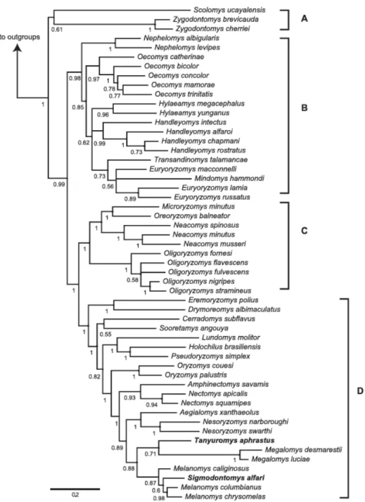
Subsequent hypotheses (PERCEQUILLO et al., 2011; PINE et al., 2012) consistently recovered the same 4 clades which were named A, B, C and D (Figure 1).
The clade A includes the genera Scolomys (2 species) and Zygodontomys (2 species). Clade B includes the most diverse genera of the tribe, Euryoryzomys (6 species), Oecomys (14 species), Handleyomys (2 species), Hylaeamys (7 species), Transandinomys (2 species) and Nephelomys (14 species; sensu MUSSER et al., 2005; PERCEQUILLO, 2015). Clade C includes few genera with numerous species: Microryzomys (2 species), Oreoryzomys (1 species), Neacomys (7 species) and Oligoryzomys (22 species). Clade D exhibits several monotypic genera, being formed by Eremoryzomys (1 species), Drymoreomys (1 species), Cerradomys (7 species), Sooretamys (1 species), Lundomys (1 species), Holochilus (6 species), Pseudoryzomys (1 species), Oryzomys (4 species), Amphinectomys (1 species), Nectomys (4 species), Aegialomys (2 species), Nesoryzomys (5 species), Tanyuromys (1 species), Melanomys (3 species) and Sigmodontomys (1 species).
The genus Mindomys (1 speices) is an insertae sedis and have never been used in molecular analysis, only in morphological ones or combines molecular and morphology dataset phylogenies. The genus is sometimes included in clade B, closely related to the genus Oecomys or Euryoryzomys and sometimes it is placed as the first split in Oryzomyini (WEKSLER, 2006; PERCEQUILLO et al., 2011; PINE et al., 2012). It is important to notice that the relationships between Oryzomyini genera are highly variable in the aforementioned phylogenies.
Recently, Machado et al. (2014) proposed a phylogeny for Oryzomyini clade D. They found that tetralophodont forms of clade D are paraphyletic and the trans-Andean taxa mostly dispersed from the cis-Andean region. The migrations routes were most likely in extreme northern South America and the Andes should operate as a post-dispersal barrier.
20
Figure 1 - Bayesian tree of Oryzomyini tribe obtained with nuclear, mitochondrial and morphological characters by Pine et al. (2012, p. 855, fig. 1)
Even though some new taxa were described or revalidated in the past few years for the Forest clade genera (PATTON et al., 2000; VOSS et al., 2001, EMMONS; PATTON, 2005; WEKSLER et al., 2006; CARLETON et al., 2009; BRENNAND et al., 2013); some clades still needs revision, as the genus Oecomys for example, once its species delimitations remains unclear.
Included into this taxonomic and phylogenetic scenario, the genus Hylaeamys was described by Weksler, Percequillo and Voss (2006) for the species formerly associated with the Oryzomys “capito complex” or to the megacephalus group (genus Oryzomys, sensu MUSSER et al., 1998; WEKSLER et al., 1999; PATTON et al., 2000; WEKSLER, 2006). The species that currently comprise the genus Hylaeamys were synonymized with Oryzomys capito by Hershkovitz (1960) and posteriorly recognized as subspecies of Oryzomys capito by Cabrera (1961), besides other taxa presently allocated into other Oryzomyini genera. Musser et al. (1998) reviewed the Oryzomys “capito complex”, and they recognized two different species groups that would be later recognized as genus Hylaeamys: the “yunganus group” with O. yunganus and O. tatei as belonging species; and “megacephalus group”, including O. megacephalus and O. laticeps. Subsequently, other species were described and assigned to the O. “capito complex” (sensu MUSSER et al., 1998). O. seuanezi was described by Weksler et al. (1999) in the eastern Atlantic Forest in Brazil, Patton et al. (2000) designated the western Amazon populations of O. megacephalus as O. perenensis and O. acritus was described by Emmon and Patton (2005) in eastern Bolivia. Weksler et al. (2006) attributed seven species to the genus Hylaeamys, named: H. acritus (Emmons and Patton, 2005), H. laticeps (Lund, 1841), H. megacephalus (Fischer, 1814), H. oniscus (Thomas, 1904), H. perenensis (Allen, 1901), H. tatei (Musser, Carleton, Brothers and Gardner, 1998) and H. yunganus (Thomas, 1902). More recently, Brennand et al. (2013) provided a new arrangement for the Atlantic Forest species of the genus. They formally recognized H. oniscus and revalidated H. seuanezi (Weksler, Geise and Cerqueira, 1999), for the species from the eastern Brazilian Atlantic Forest, assigning laticeps (Lund, 1841) as a junior synonym of H. megacephalus. However, despite a relatively good understanding of the taxonomy of the genus, Percequillo (2015) pointed out the fact that the delimitation and distribution of the species, as well the geographic variation within the genus remains unclear.
22
from H. megacephalus and H. laticeps, and treated them as two different species group (as mentioned above).
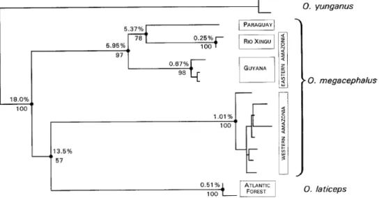
Figure 2 - Maximum Parsimony tree presented by Musser et al. (1998, p.27, Fig. 6) with O. capito complex species showing the average percent sequence divergence in the top of the nodes
24
Figure 4 - Phylogeographical relationship and geographical distribution of Hylaeamys species obtained by Costa (2003, p. 79, Fig. 7)
Figure 5 - Maximum Parsimony tree presented by Emmons and Patton (2005, p. 3, Fig. 1) when they describe H. acritus
26
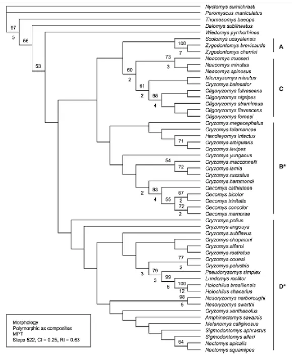
Figure 6 - Maximum Parsimony tree using morphological character presented by Weksler (2006, p. 62, Fig. 34)
Figure 7 - Partial most Parsimonious tree show by Percequilo et al. (2011, p. 337, Fig. 7) using molecular and morphological combined dataset
Figure 8 - Partial Likelihood tree presented by Percequillo et al. (2011, p. 374, Fig. 8) using only molecular dataset
28
be important to establish the monophyly of the genus and its relationship with the other genera into the clade. It would also allow advancing hypotheses on the evolutionary and biogeographic history of this clade. It is likely that more comprehensive datasets would be extremely useful to establish robust phylogenetic hypotheses for Hylaeamys genus and the Forest Clade members.
Along the years, the methods used for taxonomists to recognized species varied a lot. The concept of species has been central in Biology and the species still considered the fundamental unit of biological studies in many different aspects as anatomy, behavior, genetics, molecular biology, physiology, phylogeny, systematics, and paleontology (SOKAL; CROVELO, 1970; WIENS; PANKROT, 2002; SITES; MARSHALL, 2003, 2004; DE QUEIROZ, 2005). The biological species concept was first proposed based on evolutionary theory with the contribution of Theodosius Dobzhanski, Ernest Mayr and George Gaylord Simpson in the 1930’s and 1940’s. In this concept, the species is defined as a group of interbreeding natural populations, reproductively isolated from other groups, thus constituting a reproductive entity (MAYR, 1964; FUTUYMA, 1992). According to Mayr (1963, 1964), all differences between species are subject to geographic variation, and these differences, whether morphological, physiological or ecological, are mechanisms potentially insulators that reinforce the discontinuity between two populations. Geographic variation is then capable of producing the two components of speciation: the development and the establishment of divergence between different forms of discontinuity. Also according to this author, the speciation phenomenon is not abrupt but gradual and continuous, and we can find in nature all levels.
For a long time, biologist recognized species based in morphological methods only. Sokal and Crovelo (1970) argumented that the decisive criterion of the biological species concept proposed by Mayr (1963) is not the fertility of individuals but the reproductive isolation of populations. In that way, the existence of gaps in the pattern of phenetic diversity can be taken as evidence for reproductive isolation, and species could be delimitated based in morphological discontinuities (SOKAL; CROVELO, 1970; SITES; MARSHALL, 2004, ZAPATA; JIMENEZ, 2012). By this mean, geographic variation is then capable of producing the two components of speciation: the development and the establishment of divergence between different forms of the discontinuity.
monophyletic groups, not through reproductive barriers (ALEIXO, 2007). However, it was inevitable that the classification of organisms, according to their morphological similarities, combined with aspects of its ontogenetic development and their geographical distribution, have been, sooner or later associated with the discovery of their different degrees of phylogenetic relationship and thus, the evolutionary theory (HENNING, 1965). Through the process of speciation, a population has one or more evolutionary novelties, which can be fixed from the genetic level to morphological, biochemical and behavioral (CRACRAFT, 1989).
Using the phylogenetic species concept, the species becomes the entity of evolutionary theory and the basis for historical patterns of taxonomic diversity (CRACRAFT, 1989). Several criticisms of the phylogenetic species concept have been suggested based on the uncomfortable adjustment between its theoretical basis and its applicability (COLLAR, 1997; AGAPOW et al., 2004). Based on this discrepancy between theory and their ability to be really tested, Queiroz (1998) draws a distinction between specie concept and specie criterion. The author emphasizes that the conceptual differences that highlighted the distinctions between the different species concepts are related only to the emphasis that each one of them draws from a different phenomenon accompanying the cladogenesis process, and there is a conflict related to the type of entity to which they refer.
30
2 OBJECTIVES
Based on these hypotheses above cited, I proposed to answer the following questions: How many groups can I recognized inside the genus Hylaeamys using skull morphometric data? Can I recuperate theses morphometric groups using phylogenetic methods? Is Hylaeamys a monophyletic group? Who is the sister group of Hylaeamys into the Forest clade? These morphometric and phylogenetic groups corresponded to the current species? For answer these questions I established the following objectives:
Describe the morphometric variation between skull samples, in order to establish the discontinuities among populations of Hylaeamys;
Stablish geographical limits distribution for the morphometric groups;
Test the monophyly of the genus Hylaeamys;
Recover the relationship between the genera of the Forest clade of the tribe Oryzomyini;
Compare groups founded with morphometrical approach to those founded in the phylogenetic approach;
3 METHODS 3. 1 Sampling 3.1.1 Specimens
I analyzed the skins, skulls, of 2.411 and some skeletons and carcasses preserved in fluid of specimens of genus Hylaeamys, deposited in the following collections:
AMNH - American Museum of Natural History (New York, USA) BMNH – The Natural History Museum (London, England)
FM - Florida Museum of Natural History, University of Florida (Gainesville, USA) FMNH – The Field Museum (Chicago, USA)
INPA - Instituto Nacional de Pesquisas da Amazônia (Manaus, Brazil)
MN - Museu Nacional da Universidade Federal do Rio de Janeiro (Rio de Janeiro, Brazil)
MNHN – Musée National d’Histoire Naturelle de Paris (Paris, France)
MPEG - Museu Paraense Emilio Goeldi - Material under the supervision of Professor Claudia Nunes at Universidade Federal do Pará (Campus Bragança, Brazil)
MPEG – Museu Paraense Emílio Goeldi (Belém, Brazil)
MVZ – Museum of Vertebrate Zoology, University of California (Berkeley, USA) MZUSP – Museu de Zoologia da Universidade de São Paulo (São Paulo, Brazil) UFMG - Universidade Federal de Minas Gerais (Belo Horizonte, Brazil)
UFPB – Universidade Federal da Paraíba (João Pessoa, Brazil) UFPE – Universidade Federal de Pernambuco (Recife, Brazil) UnB – Universidade de Brasília (Brasília, Brazil)
UNEMAT - Universidade Estadual do Mato Grosso (Nova Xavantina, Brazil) UNMSM - Universidad Mayor de San Marco (Lima, Peru)
USMN - National Museum of Natural History, Smithsonian Institution (Washington, USA)
UZM – Universitets Zoologisk Museum (Copenhagen, Denmark)
34
3.1.2 Measurements
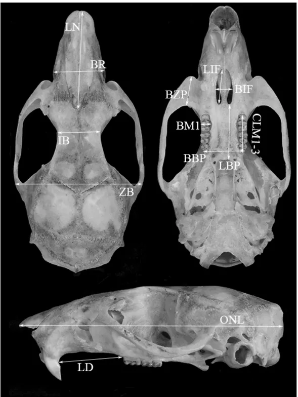
Specimens were measured following cranial and dental dimensions adapted from Voss (1988) and Musser et al. (1998) using a digital caliper to the nearest 0.01 mm. The following measurements were taken:
Occipital Nasal length (ONL): measured from the anteriormost end of the nasal to the occipital bone;
Length of diastema (LD): measured from the crown of the first upper molar to the inner side of the base of the upper incisor, on the same side of the skull;
Crown length of maxillary toothrow (CLM1-3): measured from the anterior surface of the first upper molar to the posterior surface of the third upper molar, at the crown of the molars;
Breadth of first upper molar (BM1): breadth of the first upper molar, measured on the basal portion of the molar crown, at the level of the paracone-protocone pair;
Length of incisive foramina (LIF): the greatest length measured from the anterior to the posterior edge of the incisive foramen;
Breadth of incisive foramina (BIF): the greatest internal breadth, measured on the lateral margins of the incisive foramen;
Breadth of bony palate (BBP): the greatest breadth of bony palate measured across the third upper molar;
Breadth of rostrum (BR): measured across the rostrum at the posterior extremity of the upper edge of the infraorbital foramen;
Length of nasals (LN): measured from the anteriormost end of the nasal to the naso-frontal suture;
Length of bony palate (LBP): measured from the posterior margin of the incisive foramen to the anterior margin of the mesopterygoid fossa;
Interorbital breadth (IB): shortest distance through the frontals in the orbital fossa; Greatest zygomatic breadth (ZB): greatest external distance of the zygomatic arches, close to the squamosal roots, measured across the skull;
Breadth of zygomatic plate (BZP): the shortest distance between the anterior and posterior margins of the inferior zygomatic root or zygomatic plate.
Figure 9 - Dorsal, ventral and lateral views of a skull of a specimen of Hylaeamys (UFPB BC195), from Murici, Alagoas state, Brazil, showing the limits of cranial and dental dimensions measured in the specimens studied (see text for definitions and abbreviations)
3.1.3 Sexual dimorphism
36
(CARLETON; MUSSER, 1989, 1995; MUSSER et al., 1998; CARMADELLA et al., 1998; PRADO; PERCEQUILLO, 2011; ABREU-JUNIOR et al., 2012; BRENNAND et al., 2013). Therefore, females and males are combined in all subsequent morphologic and morphometric analyzes.
3.1.4 Age criteria
I employed five different age classes defined based in eruption and wear of superior molars, following Voss (1991) and Percequillo (1998). The classes are described as follows and only adults were used in the morphometric and morphological comparisons, but all age classes were used to described the valid species:
Age class 1 (AC1): first (M1) and second (M2) superior molars with no apparent wear. Anteroloph, mesoloph and posteroloph are distinct and easily recognizable. The third superior molar (M3) are not erupted or newly erupted with main cusps still closed, labial lophs well developed and isolated, labial and lingal flaxus deep and distinct (Figure 10A).
Age class 2 (AC2): M1 and M2 with a small tooth wear, exhibiting a small part of dentine between cusps. M3 already showing minimal to moderate wear; anteroloph and mesoloph may be connected to paracone, through marginal lophules, posteroloph nearly fused to metacone marginally (Figure 10B).
Age class 3 (AC3): M1 and M2 with moderate wear. M3 with marked wear and a nearly flat surface, anteroloph and mesoloph fused marginaly to paracone forming a long anterofosset end a mesofosset respectively; posteroloph completely fused to metacone forming a distinct mesofosset (Figure 10C).
Age Class 4 (AC4): M1 and M3 with a heavy wear, showing indistinct and massive exposure of dentine. M3 appears quite flat, with major exposition of dentine; anteroloph, mesoloph and posteroloph indistinct and fused to major cusps (Figure 10D).
Figure 10 - Five different age classes (AC1, AC2, AC3, AC4 and AC5 respectively), based on molar eruption and wear; root exposition is also useful to determine age, with classes 4 and 5 with moderate and large exposition of dentine, respectively
3.1.5 Anatomy
Anatomical terminology used in this study follow different authors. I followed Hershkovitz (1977), Voss (1988), Carleton and Musser (1989) for external features, and Hill (1935), McDowell (1958), Wahlert (1974, 1985), Voss (1988), Bugge (1970), Guthrie (1963) and Steppan (1995) for cranial and dental terms.
3.1.6 Gazetteer
Localities and geographical coordinates were taken from the original and museum labels attached to specimens; when geographical coordinates were not available, I used other sources (GEONAMES, 2004; PAYNTER; TRAYLOR, 1991; U.S. BOARD ON GEOGRAPHIC NAMES, 1994). The gazetteer is ordered alphabetically by country, state or province and collection locality. All maps produced in this study using QGIS 1.8 (2012) are numbered according this gazetteer. The gazetteer is presented in Appendix A.
3.2 Assessment of geographical variation 3.2.1 Hylaeamys Groups of species
38
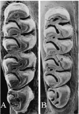
Figure 11 - Occlusal views of right upper molar rows from species of Hylaeamys adapted from Musser et al. (1998, p. 77, Figure 30) showing labial (lf) fossettes and paraflexus (p) in the second molar. A: H. yunganus (AMNH23166) from Peru (CLM1-3 = 5 mm). B: H. perenensis (AMNH 231655) from Peru (CLM1-3 = 5 mm)
These samples were grouped to yield more robust samples by increasing the number of specimens per group. I delimitated some sub-groups based on the geographic proximity criterion, karyotype information, the criterion of similarity between the geomorphological characteristics of the samples (riverbanks, mountain slopes, relief), the similarity between qualitative external characters and cranial characters; morphological and genetic differences reported in the literature (MUSSER, 1968; VANZOLINI, 1970).
I applied multivariate tests among these groups. As the genus is wildly distributed in South America biomes, I started the comparisons between the groups by biomes. For the Amazon Forest, I also used the large rivers as a tool for delimited the internal groups. Moreover I did a specific comparison for groups in sympatric areas, such as Bolivia.
3.2.2 Karyotype variation
3.2.3 Statistics Analyses for Cranial Morphometric variation
The samples are distributed in all Cis-Andean South America biomes and all analyses of geographic variation were conducted in pooled samples within and between those two groups (see 3.2.1 for more details).
Standard descriptive statistics (mean, standard deviation and observed range) have been calculated for all groups with more than five adults. Dice-Leraas univariate diagrams using mean and confidence intervals (95%) for each cranial and dental variable was used to assess geographic variation comparisons between samples.
A Principal Component Analysis (PCA) over the within-group variance-covariance matrix and a Discriminant Functions Analysis (DFA) were computed using the cranial and dental log-transformed variables between groups. The first two or three principal components and discriminant function were plotted in a scatterplot graphic, providing visual observance of the patterns. SPSS (SPSS, 2008) was used to perform all statistics analysis.
3.3 Phylogeny
3.3.1 Extractions and Hybrid enrichment
The DNA was extracted using Invitrogen PureLink Pro 96 kit, following the kit recommended procedures. For DNA from skin samples some changes in the digestion step were done, adding more 20uL of protease, computing a total of 40ul of protease, 5ul of DTT and the time of digestion were overnight or more than 16 hours. The DNA was quantifying using nanodrop, and only samples with a minimum of 10ng/µl could be submitted to Library preparation.
The Hybrid enrichment consists in the development of probes that will be hybridized to a DNA library, isolating the targets from the genome prior to high-throughput sequencing (LEMMON; LEMMON, 2013; McCOMACK et al., 2013). The procedure was made at Center For Anchored Phylogenomics at Florida State University following the methods developed by Lemmon, Emme and Lemmon (2012). It consists in a mix of probes that capture a conserved DNA region flanked by less conserved region across the genome and generating up to 3000 bp per locus. After enrichment, samples were sequencing on Illumina HiSeq2000 at the Florida State University Translational laboratory.
3.3.3 Alignment and Phylogenetic analysis
40
using MUSCLE (EDGAR, 2004), implemented in Geneious 5.1 (DRUMMOND et al., 2012). Alignments were manually inspected and all ambiguous regions or missing sites were denoted as charcter sets using MacClade 4.08 (MADDISON; MADDISSON; 2005) and excluded from phylogenetic analysis.
For phylogenetics analysis, only one of the alleles alignments was used. The alignment has 7.24% of proportion of gaps. The Maximum Likelihood tree was obtained using RaxML-HPC 8.0 (STAMATAKIS, 2014) implemented in CIPRES science geteway. A GTR GAMMA model of rate heterogeneity was estimated using 322 data partitions with join branch length optimization and 1000 bootstrat were performed.
Samples from clade D of Oryzomyini tribe were used as outgroup and a sample of Abrawayomys ruschii was used to root the tree. The trees were edited using FigTree 1.4 (STAMATAKIS, 2014).
3.4 Species Delimitation
To recognize and define diagnosable groups and test their reciprocal monophyly, and formalize hypothesis about the species of the genus Hylaeamys, I combined the results of geographical variation among samples and karyotype information available in the literature, altogether with the phylogenetic trees. All this information was the core evidence to support my taxonomic decisions and delimitations of the taxa. In this sense, I employed the integrative approach to establish these species, that although is not a formal species concept, it considers the use of different methods to recovery a lineage, applying the criteria of diagnostic characters and reciprocal monophyly to recognize species. (DE QUEIROZ, 1998, 2007; COLLAR, 1997; CRACRAFT, 1989; PADIAL et al., 2009)
3.4.1 Species Account
4 RESULTS
4.1 The “yunganus group”
The samples of this group included specimens with two fosettes (a labial and a medial fossette) and a short paraflexus in the second upper molar (Figure 11). Presently, two species are recognized into this group: H. tatei (Musser, Carleton, Brothers and Gardner 1998) and H. yunganus (Thomas 1902). These two species are sympatric with others forms of group “megacephalus” of genus Hylaeamys: H. yunganus presents a wide distribution in the northern portion of South America in both banks of Rio Amazonas, and part of central Brazil and Bolivia, while H. tatei exhibits a restricted distribution in few localities of central Ecuador, on the eastern slope of Eastern Andean Cordillera (Figure 13; see detailed maps with localities numbers in the topic Species Account, associated to each recognized species).
Figure 12 - Distribution of all samples of “yunganus group” analyzed. Open circles are samples presently named as H. yunganus, dark circles are samples presently named as H. tatei
4.1.1 Morphometric variation
42
both approaches, I also considered the karyotype information (topic 4.1.2) and previous molecular results published elsewhere (MUSSER et al., 1998; PATTON et al., 2000; JORGE-RODRIGUES, 2011) to delimit the pooled samples.
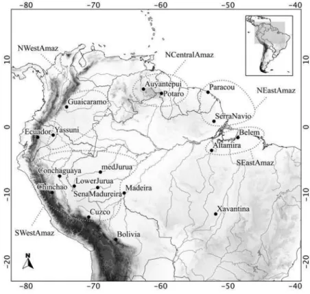
At first, I pooled the samples through the geographic proximity criteria and assembled 17 groups with at least 4 individuals per group: these groups were listed in the Table 1, in the column labelled group 1 (they are also represented in Figure 14). Secondly, these 17 previous groups were polled according to the following criteria: the margin of the Rio Amazonas, the geographic distance between them and the morphology of specimens (Figure 14). These nine new groups of samples, labelled group 2 (on Table 1) were named as: NEastAmaz, NCentralAmaz, NWestAmaz and Ecuador for samples in the north of Rio Amazonas; SEastAmaz, Xavantina, Bolivia, Madeira, SWestAmaz for samples in the south of Rio Amazonas (Figure 13). Specimens from Xavantina were placed in a separated group because represents a transitional area between Amazon Forest and Cerrado biome.
To be able to better analyze the geographic variation within “yunganus group”, I performed the statistic analysis using only the group 2 of samples once this groups had a larger number of individuals and consequently showed more robust statistics results.
The Bolivia sample will be used in a subsequent analysis with others samples from that geographic region (topic 4.2.1.1) with the objective to better identify and delimit the discontinuities among Hylaeamys samples from this area. The samples from localities 251 (Mera, Pastaza, Ecuador) and 260 (Palmera, Tungurahua, Ecuador) were joined and labeled as Ecuador because this population presents specific cranial and dental characteristics that distinguished them to the others samples, and were formally recognized as O. tatei (MUSSER et al., 1998).
Table 1 - Pooled localities (Groups 1 and 2) and their respective localities number and total number of specimens of “yunganus goup” used in morphological and morphometric analysis. The localities numbers are those from the Gazetteer presented in Appendix I
Group 1 Group 2 Localities specimens in Number of
group 1
SerraNavio NEastAmaz 67, 68 16
Paracou NEastAmaz 265 7
Auyantepui NCentralAmaz 386, 391 7
Guaicaramo NWestAmaz 234, 236, 237, 238 6
Yasuni NWestAmaz 233, 243, 244, 247, 252, 255 16
Conchaguaya SWestAmaz 326, 327, 360 4
Chinchao SWestAmaz 314, 348, 352, 354 12
Potaro NCentralAmaz 269, 279 6
BaixoJurua SWestAmaz 53, 54, 55, 56, 59 24
MedJurua SWestAmaz 73, 76, 78, 82, 85, 86, 91 20
SenaMadu SWestAmaz 52, 57, 362 14
Cuzco SWestAmaz 306, 310, 311, 312 6
Bolivia Bolivia 1, 11, 35, 37, 49, 221 8
Madeira Madeira 37, 49, 221 5
Xavantina Xavantina 140 15
Altamira SEastAmaz 185, 190, 194 197 7
Ecuador Ecuador 251, 260 7
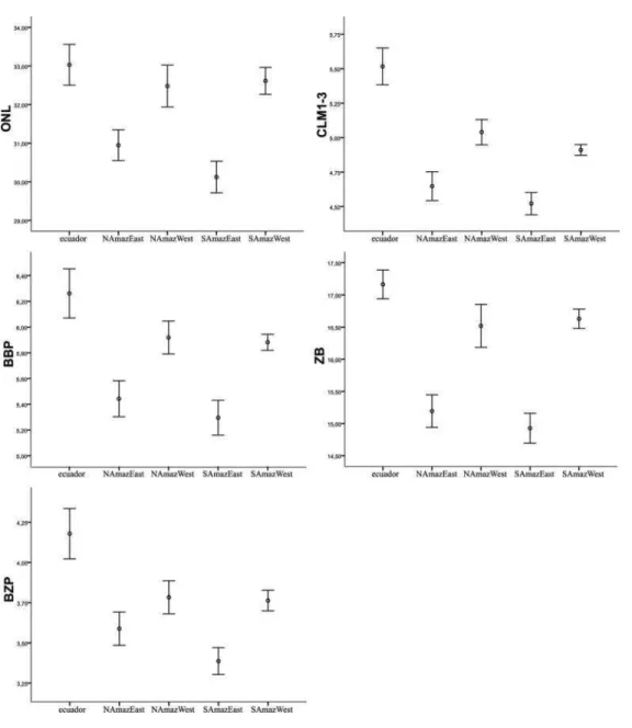
To explore data, I performed error bar diagrams, to compare the means between all samples simultaneosly. I did not include the samples Bolivia and Madeira in the graphics because they had a small number of specimens, who influenced the confidence interval, but these groups were used in the multivariate tests. For the variables ONL, CLM1-3, BBP, ZB and BZP we could observe tree distinct groups: Ecuador, Eastern Amazon Forest and Western Amazon Forest (Figure 14). In the other hand, for the variable BM1 (Figure 14) the sample from Ecuador have the largest mean value, but the differences between the means from Eastern and Western samples are not quite distinct.
44
Figure 14 - Comparison of variables ONL, CLM1-3, BBP, ZB and BZP between samples of “yunganus group”. Open circles are the mean and error bar diagrams showing 95% of confidence interval for each group
Figure 15 - Comparison of variable LD between samples of “yunganus group”. Open circles are the mean and error bar diagrams showing 95% of confidence interval for each group
Figure 16 - Comparison of variables LN, BIF and LIF between samples of “yunganus group”. Open circles are the mean and error bar diagrams showing 95% of confidence interval for each group
46
Figure 17 - Comparison of variables IB, LBP and BR between samples of “yunganus group”. Open circles are the mean and error bar diagrams showing 95% of confidence interval for each group
In the most of the variables, we could observe that the samples from both sides of Amazon River had the same mean and the differences were more conspicuous between Eastern and Western populations, instead of Northern and Southern populations of Amazon Forest.
Table 2 - Values of first (PC1), second (PC2) and third (PC3) components resulted from a Principal Component Analysis of log transformed cranial and dental variables of Hylaeamys “yunganus group”. Variables with highest scores are in bold
Variables PC1 PC2 PC3
ONL 0.882 0.067 0.351
LD 0.711 0.065 0.510
CLM1-3 0.803 0.057 -0.318
BM1 0.643 0.038 -0.699
LIF 0.506 -0.716 0.031
BIF 0.493 -0.653 0.158
BBP 0.763 -0.079 -0.306
BR 0.540 -0.004 0.496
LN 0.639 0.075 0.384
LBP 0.639 0.075 0.384
IB 0.595 0.285 0.137
ZB 0.892 0.001 0.116
BZP 0.705 0.338 -0.189
Eigenvalue 0.005 0.002 0.001
% Variance 45 14.99 12.6
48
Figure 18 - Samples score, based on log-transformed mean value of 13 cranial and dental measurement projected onto the first and second principal components (PC1 and PC2) extracted from analysis of samples of “yunganus group” listed in Table 1 and labeled as group 2
Table 3 - Values of first (DS1), second (DS2) Discriminants Scores resulted from a Canonical Discriminant Analysis of cranial and dental log transformed variables of Hylaeamys “yunganus group”. Variables with highest discriminant score are in bold
Variables DS1 DS2
ONL 0.474 -0.593
LD 0.273 -0.641
CLM1-3 0.449 0.096
BM1 0.611 0.793
LIF 0.242 -0.103
BIF 0.208 -0.127
BBP 0.333 0.124
BR 0.356 -0.426
LN 0.300 -0.370
LBP 0.146 -0.349
IB 0.183 -0.250
ZB 0.736 -0.677
BZP 0.396 -0.036
Wilk’s Lambda 0.000 0.000
Eigenvalue 4.525 0.558
50
Figure 20 - Scatterplot of first and second Canonical Score of log-transformed value of 13 cranial and dental measurements extracted from a discriminant function analysis with covariance matrix of samples of “yunganus group” listed in Table 3 and labeled as group 2 of Table 1
4.1.2 Karyotypic variation of “yunganus group”
Gardner & Patton (1976) described three different karyotypes for Hylaeamys populations from Peru. One was assigned to Oryzomys capito (see Karyotype of “megacephalus group” (topic 4.2.1 for more details) and two were assigned to Oryzomys yunganus. The authors named these specimens according to skull characteristics and comparisons with the holotype of O. yunganus deposited at The Natural History Museum (Britsh Museum).
The first karyotype is 2n = 60 and FN = 66, comprising four pairs of metacentric, 25 pairs of acrocentrics, and two sex chromosomes: a large acrocentric X and a medium or small acrocentric Y. This karyotype was found in populations of Ayacucho department, (locality San José, Rio Santa Rosa). The second karyotype is 2n = 58 and FN = 62 and is identical in form to the previous one except for the absence of one pair of small metacentric chromosomes. This karyotype was found in populations of Loreto department (at the locality of Balta, Rio Curanja).
could not really identify at specific level but they attribute that polymorphism to a macconnelli-capito complex. However, what intrigued the researchers was the fact that each individual has a unique karyotype and concludes that the Trafelberg sample represented the greatest amount of chromosomal polymorphism thus far identified in a single naturally occurring mammalian population.
Kerridge and Baker (1990) documented that the sample from Tafelberg consisted of two different species: Oryzomys capito and Oryzomys yunganus. The O. capito samples had FN = 58 - 59 and the FN for O. yunganus ranged from 64 to 67. But the authors also emphasized that the removal of two specimens of O. capito in that sample reduces the variation in FN but all the fusions identified by G-bands remain assigned to one species, O. yunganus, and the polymorphism is still greater than that described of any other occurring population of mammals. The observation of the absence of O. capito alleles in the samples of chromosomally polymorphic O. yunganus is not compatible with the hypothesis that chromosomal polymorphism resulted from recent hybridization between the O. capito and an unidentified species.
In their manuscript about the “Oryzomyscapito complex”, Musser et al (1998) presents the karyotype 2n = 58 and FN = 62, obtained in the Brazil (in Juruá River, a tributary of Amazon River in northwestern Brazil) for the O. yunganus populations. This karyotype was more detailed by Patton et al. (2000) in their manuscript about small mammals of the Juruá River. The karyotype of this population from the western part of Amazon Forest agree with those previously described by Gardner and Patton (1976) for the populations from Peru. Patton et al. (2000) describe this karyotype as 25 pairs of large to small acrocentric, 3 pairs of small metacentric and two sex chromosomes: a medium large acrocentric X and a small acrocentric Y.
In 2000, Volobouev and Aniskin presented a karyotype of a female O. yunganus from Loreto department in Peru as a tree pairs of small metacentrics, 25 pairs of acrocentrics decreasing in size and a couple of medium size acrocentric X, resulting in 2n = 58 and FN = 62. This karyotype agrees with those previously described by Gardner and Patton (1976) from Ayacucho department, also in Peru and those described by Patton et al. (2000) from northwestern Brazil.
52
So, the karyotype diversity registered for this group is compounded by the following different karyotypes (Figure 21): 2n=60, FN=66 from Peru; 2n=58, FN=62 from Peru and northwestern Brazil; 2n=60, FN=62 from central Brazil and 2n=52-59; FN=64-67 from Suriname.
Figure 21 - Distribution of the karyotypes described for populations of Hylaeamys “yunganus group”
Unfortunately, the karyotypes for most part of the samples that I analyzed were not available in the literature. In addition, I did not have access to the specimens from Niquelândia with karyotype 2n = 60, FN = 62, so, these specimens were not included into the morphometric analysis, and have not their identity checked.
4.1.3 Summary of variation in “yunganus group”
The morphometric analyses of variation showed sharp differences in the skull size, revealing gaps between eastern (NEastAmaz, SEastAmaz, Xavantina and part of the specimens of the sample Madeira) and western (NCentralAmaz, NWestAmaz, SWestAmaz, Bolivia and part the specimens from Madeira) populations from both sides of Amazon River, and finally and most noticeably, regarding the Ecuador pooled sample. For a better definition and classification of samples from Madeira, this sample will be included as an independent group in subsequent morphometric comparisons (Bolivia samples, and Amazon Forest groups).
Musser et al. (1998) were the first to highlight the morphometric geographic variation observed into this “yunganus group”. These authors also described the species H. tatei, based in some specimens collected in Ecuador, more exactly, in two localities: Mera (locality number 251 in the Gazetteer in Appendix I) and Palmera (locality number 260 in the Gazetteer in Appendix I). Despite the restricted distribution of the taxa in only central and northern Ecuador, these authors presented morphological and morphometric differences between H. tatei and H. yunganus. They also highlighted the occurrence of geographic variation among populations of H. yunganus.
In my results I was able to analyze more material than Musser et al. (1998), and, consequently, increase the number of specimens and localities employed in the analysis. With larger sampes, the discontinuities between eastern and western populations appeared more conspicuous, as well as the differences between those and the sample that I labelled as Ecuador.
These specimens from Ecuador showed morphometric difference in the total size (length and breadth) of the skull, as well as in the breadth of M1 and length of maxillary tooth row (Figure 14). These characteristics were also visible in qualitative aspects, along with other traits, as more robust skulls; posterior part of zygomatic plate positioned more perpendicular to the anterior - posterior axis of the skull; supraorbital margins sharp and moderately beaded. However, no information was founded in the literature about karyotype for that sample.
54
However, for the others samples of “yunganus group” the morphometric analyzes highlighted an important geographic variation. Populations from eastern Amazon Forest presented difference from the populations on the western part of the Biome. The eastern populations represented by populations from NAmazEast, SAmazEast and Xavantina showed a delicate skull and the smallest means for the variables related to length and breadth of the skull, as well as the breadth of M1 and length of maxillary tooth row (Figure 14). Samples from Madeira had a smaller and more gracile skull, more similar to eastern poulation samples. Jorge-Rodrigues (2013), in a previous analysis of Hylaeamys yunganus, also showed morphological and morphometric difference between population from Guiana and populations from Rio Juruá and western Amazon Forest. The author considered those differences as geographical variation of this species, as well as Musser et al (1998). I think that the variation between those samples from east and west of Amazon Forest are really expressive, and depending upon the results of the phylogenetic analysis, can be translated to the recognition of a new biological entity in the group.
4.2 The “megacephalus group”
The samples of this group included specimens with one fossette and a long paraflexus in the second upper molar (Figure 11). At the present, five species are recognized into this group: H. acritus (Emmons and Patton 2005), H. laticeps (Lund 1841), H. megacephalus (Fischer 1814), H. oniscus (Thomas 1904), H. perenensis (Allen 1901). They are distributed into the north part of Cis-Andean South America, going eastern until the Brazilian coast through the entire central Brazil and going south until Paraguay (Figure 21).
4.2.1 Cranial morphometric variation of “megacephalus group”
Figure 21 - Distribution of the known collection localities of all samples of “megacephalus group”
4.2.1.1 Bolivia samples
56
Therefore, it is not quite clear how many species occur in Bolivia, nor their geographic distribution.
I made some morphometric analysis with all samples from Bolivia, including specimens of “yunganus group” from Bolivia to analyze the variation into the skull size of that populations. I also used samples from close localities from Central Brazil and Paraguay, and samples from Madeira River and Peru (Table 4) to better understood the variations of the Bolivian samples (Figure 22) and to propose a better delimitation of the taxa in that region.
Table 4 - Grouped localities and their respective localities number (numbers correspond to gazetteer in Appendix I) and total number of specimens of Hylaeamys used in morphometric analysis of Bolivia samples
Groups Localities Number of specimens
in each group
Bodoquena 164, 165, 166 14
Baures 10 6
Centenela 8, 12, 14 9
CostaMarq 15 15
Elrefugio 17, 18 7
EBBeni 13, 19, 26 7
Madeira 221 8
OppCostaMarq 3, 9, 24 17
Paraguay 281, 282, 283, 287,
288
20
Paranatinga 144, 137 12
PNKempf 42, 44, 45 8
RioPitasama 2, 27, 39, 41, 46, 47, 49
10
PuertoSiles1 4, 5, 22 3
yunganus 1, 37, 35, 41, 40 5
1. Samples from Puerto Siles were not included into univariate analysis because of the small number of specimens
PuertoSiles and from “yunganus group” into the graphics because they had a small number of specimens (Table 4) that influenced the confidence interval.
Figure 22 - Distribution of the samples of Hylaeamys groups in Bolivia, Brazil and Paraguay, employed in the quantitative analyses of variation
58
60
Figure 25 - Comparison of variables IB, BZP and LBP between samples from Bolivia. Open circles are the mean and error bar diagrams showing 95% of confidence interval for each group
Table 5 - Values of first (PC1), second (PC2) and third (PC3) components resulted from a Principal Component Analysis of log transformed cranial and dental variables of Hylaeamys from Bolivia. Variables with highest scores in each component are in bold
Variables PC1 PC2 PC3
ONL 0.924 -0.041 -0.098
LD 0.893 0.036 -0.130
CLM1-3 0.428 -0.029 0.041
BM1 0.141 0.029 0.024
LIF 0.729 0.069 0.323
BIF 0.606 0.445 0.571
BBP 0.366 0.742 -0.390
BR 0.504 -0.066 0.425
LN 0.805 0.063 -0.401
LBP 0.614 -0.154 -0.186
IB -0.090 -0.018 0.416
ZB 0.885 0.061 -0.045
BZP 0.709 -0.622 -0.022
Eigenvalue 0.003 0.001 0.001
62
Figure 26 - Samples score, based on log-transformed mean value of 13 cranial and dental measurement projected onto the first and second principal components (PC1 and PC2) extracted from analysis of Hylaeamys samples from Bolivia
In the Discriminant Function Analysis, the first discriminant function was responsible for 80.6% of the variation and the variables (+) BBP, (-) BZP, and (+) LN showed the highest scores (Table 6). For the second discriminant function, which was responsible for 19.4% of the variation, the following variables had the highest values: (+) BZP, (+) ONL, (+) ZB. The scores are presented in a scatterplot graphic (Figure 28).
Table 6 - Values of first (DS1) and second (DS2) Discriminants Scores resulted from a Canonical Discriminant Analysis of cranial and dental log transformed variables of Hylaeamys from Bolivia. Variables witch must influence each discriminant score are in bold
Variables DS1 DS2
ONL -0.011 0.650
LD -0.002 0.567
CLM1-3 0.002 0.257
BM1 0.128 -0.027
LIF -0.039 0.437
BIF 0.104 -0.090
BBP 0.866 0.501
BR -0.034 0.450
LN 0.178 0.588
LBP -0.074 0.417
IB 0.014 -0.090
ZB 0.090 0.613
BZP -0.388 0.922
Wilk’s Lambda 0.000 0.000
Eigenvalue 1.245 0.299
64
Figure 28 - Scatterplot of first and second Canonical Score of log-transformed value of 13 cranial and dental measurements extracted from a discriminant function analysis with covariance matrix of Hylaeamys samples from Bolivia
The dispersal of scores on the multivariate space showed some level of structure between Bolivia samples, with three main clusters recognized; one, including samples from EBBeni, RioPitasama and yunganus groups; another cluster, formed by the samples from Centenela, CostaMarq and ElRefugio; and one last cluster, that exhibit the samples from OppCostaMarq, PNKempf, PuertoSiles and Baures.
Despite the morphometric difference between samples of the first and second clusters, no qualitative trait was found for each cluster, except for the presence of the two parafossets on the specimens of the “yunganus group” samples. On the other hand, morphological characters, as a single complete dermal ring on digit I, and a notch in the rim of auditory meatus, were observed only in speciemens of the last group.
that had the highest score in second component were (+) BIF, (+) BZP and (-) CLM1-3. The scores are showed into the scatterplot graphic (Figure 29).
Table 7 - Values of first (PC1) and second (PC2) components resulted from a Principal Component Analysis of log transformed cranial and dental variables of Hylaeamys from Bolivia, Paraguay, Madeira River and nearby Central Brazil. Variables with highest scores in each component are in bold
Variables PC1 PC2
ONL 0.922 0.099
LD 0.890 0.157
CLM1-3 0.575 -0.236
BM1 0.257 -0.018
LIF 0.748 0.018
BIF 0.583 0.672
BBP 0.006 0.161
BR 0.298 0.197
LN 0.708 0.128
LBP 0.728 0.083
IB 0.015 0.164
ZB 0.845 0.162
BZP 0.776 -0.574
Eigenvalue 0.003 0.001
66
Figure 29 - Scatterplot of first and third Canonical Score of log-transformed value of 13 cranial and dental measurement extracted from a discriminant function analysis with covariance matrix of Hylaeamys samples from Bolivia, nearby central Brazil, Madeira River and Paraguay
Table 8 - Values of first (DS1) and second (DS2) Discriminants Scores resulted from a Canonical Discriminant Analysis of cranial and dental log transformed variables of Hylaeamys from Bolivia. Variables witch must influence each discriminant score are in bold.
Variables DS1 DS2
ONL 0.424 -0.208
LD 0.466 -0.366
CLM1-3 0.477 0.154
BM1 0.095 0.227
LIF 0.276 0.266
BIF 0.083 -0.088
BBP -0.305 -0.305
BR -0.205 0.097
LN 0.136 -0.174
LBP 0.507 -0.508
IB -0.141 -0.026
ZB 0.278 -0.140
BZP 0.539 0.413
Wilk’s Lambda 0.000 0.000
Eigenvalue 2.099 0.948
68
Figure 30 - Scatterplot of first and second Canonical Score of log-transformed value of 13 cranial and dental measurement extracted from a discriminant function analysis with covariance matrix of Hylaeamys samples from Bolivia, nearby central Brazil, Madeira and Paraguay
These results showed that samples from Bodoquena, Paraguay, Paranatinga and Madeira (some specimens) were morphometrically distinct from the specimens from Bolivia. It is also visible that specimens from OppCostaMarq, PNKempf, PuertoSiles and Baures were more similar, being clustered, although with some overlap to other Bolivian samples. On the other hand, the variation among the first and second clusteres described above was much less pronounced. Such results lend me to hypothesize that, aside from specimens of the yunganus group, in Bolivia there are two additional clusters (one from OppCostaMarq, PNKempf, PuertoSiles and Baures; the other from EBBeni, RioPitasama, Centenela, CostaMarq and ElRefugio), both distinct among them and also distinct to other close geographic samples from Brazil, as demonstrated above.
4.2.1.2 Amazon Samples
cases for statistics analysis and, very likely, more robust comparisons between samples, I grouped samples from group 1 according to the north and south margins of Amazon River (Figure 31), and previous analysis performed with some specimens as those from Rio Jurua (PATTON et al. (2000). These samples were labeled as indicated in Group 2 of Table 9.
As the samples from Bolivia showed to be a unique morphometric unity when compared with others samples I decided, in a first moment, to consider them as a unique sample. In a second moment, I splited them into 2 different groups according to the results founded when I analyse only Bolivian samples. That way I could better compare the variation founded into Bolivia with all others samples from Amazon Forest.