Sorting in Higher Education in Brazil
Priscilla Bacalhau
Enlinson Mattos
April 12, 2016
Abstract
This paper investigates students sorting in higher education in Brazil based on three merged databases: (i) the National Household Sample Survey (PNAD/IBGE), (ii) the National Exam of Student Performance (ENADE), and (iii) the National Survey of Secondary Education (ENEM). First, evidence indicates that family education level is an important factor in students access to higher education institutions (HEI). Each year of education for a student’s mother increases by 1.9% p.p. (0.7% p.p.) the likelihood of a student entering a public HEI. Second, the difference in students score (value added) for their field-specific ENADE scores in their first (freshman) and third years (senior) is calculated to construct a measure of HEI quality. The results suggest that students at public institutions obtain 6.17 (15%) points larger valued-added scores. Last, the Oaxaca-Blinder decomposition and general-exam scores results suggest that only 50% of the score differential can be explained by the observable characteristics of families and institutions. However, after including individual’s ENEM scores (our proxy for
talent), the model explains nearly 90% of the grade differential between public and private
HEIs. The results support that public Brazilian HEIs provide larger value-added education and attract the most talented individuals.
Keywords: Public versus private provision of education, sorting, education public policies,
qual-ity of higher education
1
Introduction
In compulsory education, families may decide to enroll their children in either the public or the
private system and do not have the opportunity to opt out. This mechanism, however, might
not work in higher education institutions (HEI), such as college or universities. Individuals can
self-select private or public education based on the expected returns and costs. The expected
returns from higher education, which drive enrollment decisions, depend on the quality of the good
provided. The decision to enter a public or private HEI then might be determined by the difference
in the quality of the education provided and the associated costs of its consumption. The aim
of this paper is to investigate the factors associated with sorting into public and private higher
education in Brazil. First, whether the public sector provides a different quality good than the
private sector is evaluated. Next, whether the quality difference between public and private HEIs
serves as a mechanism which attract different students to public HEIs is explored. Education
services, although not a pure public good, are provided by the public sector in most countries.
The public provision of basic or compulsory education can be associated with a redistributive
goal and a positive externality for individuals. In other words, governments can provide a quality
attractive only for lower-income individuals, enabling income redistribution from the rich to the
poor (Besley and Coate, 1991). In Brazil, such screening may occur in mandatory education due
to the low quality of basic public education in Brazil, as well as other countries, such as Italy
(Checci and Japelli, 2003). However, public HEIs in Brazil claim to provide better quality, so
they are not considered by members of the poorest and most vulnerable populations due to their
restrictive selection processes. 1 Usher (1977) views public spending as a redistributive instrument,
but Arrow (1971) emphasizes its ineffectiveness. 2 Researchers point out that, in the absence of
the information required to target certain benefits, self-targeting mechanisms should be devised
to induce only the intended recipients to participate and others to opt out. For instance, certain
costs (e.g., a low-quality product, workfare, time-consuming application procedures) that only the
1
See Bertola, Checci, and Oppedisano, 2007 for the Italian case.
2
targeted population is prepared to endure can be imposed on participants. Those other than the
targeted population will find the costs to be prohibitively high for a variety of reasons (see, among
others, Nichols and Zeckhauser, 1982; Blackorby and Donaldson, 1988; Besley and Coate, 1991,
1992). Boadway and Marchand (1995) identify where the use of public spending is preferable to
cash transfers. They assume that there is an available non-linear income tax and, as do Besley and
Coate (1991), that individual skills are not observable, making lump-sum transfers infeasible. Thus,
Boadway and Marchand (1995) also deal with the provision of uniform and quasi-private goods
but include the possibility of complementing private and publicly provided goods in the model.
Assuming that taxes are always adjusted to be optimal (Stiglitz, 1982), an increase in the amount
of publicly provided goods has a positive effect on social welfare as long as it makes the self-selection
constraint slack. Specifically, assuming that there are two types of individualsthose with low ability
and those with high abilityone must provide an amount higher than the individual with high ability
will accept, so that individual will prefer to consume the good provided by the private sector,
and the individual with lower skills will consume the good provided by the public sector. Besley
and Coate (1991) discuss how the public provision of private goods can be performed to achieve
redistribution purposes. Focusing on the efficiency of in-kind transfers, Besley and Coate (1991)
assume that publicly provided goods are discrete, indivisible, and provided evenly to individuals but
can be produced at either low or high quality. These goods are normal, and individuals cannot top
them of. Efficient redistribution occurs when the publicly provided good is consumed only by the
poor and by the exactly amount they are willing to pay if they received that value in cash. Thus,
redistribution might occur through uniform provision, even when funded by a lump-sum tax, but
may be generally inefficient outside the given case. Despite the potential efficiency improvements
from direct cash transfers to the poorest members of society, the cost of this instrument includes
the collection of personal income information, a non-existent problem in uniform provision, where
individuals select themselves. Grassi and Ma (2011) introduce an alternative approach focusing on
the public provision of health services. Their model claims that the government needs to ration the
consumption of publicly provided goods due to budget constraints and that rationing determines
which consumers have the right to publicly provided goods. Consumers that remain outside the
possible reactions of the private market. Two schemes of information are possible in this model.
In the first, the government needs a tool to identify individuals wealth level and, based on that
information, establish rationing and consumption: who consumes and who does not consume the
good. In this regime, the government should ration consumption by both rich and poor to reduce
the prices charged in the private market: by failing to publicly provide the good for some poor
consumers, the government makes it attractive for the private market to charge a lower price when
the cost is not high. This result conflicts with Besley and Coates (1991) finding that no poor
individuals experience rationing due to assumed self-selection. The second possible information
scheme depends on the ratio of the benefit and cost related to consumption of that good. When
cost is chosen to achieve rationing, it is most efficient to maximize the consumer surplus, so the
government has both information types (wealth and treatment cost) available for use. In this
case, rich and poor individuals are treated equally because the public provision is based on the
cost effectiveness of each customer relationship. In the context of the public provision of higher
education, the government must take into account the (private and public) benefits and costs for
individuals who wish to enroll in a public or private HEI or finding a job. Consequently, publicly
provided higher education should attract only those who gain the largest costbenefit ratio. This
pattern could provide a theoretical justification of why the government, instead of only supporting
the private sector, provides higher education, rations its supply, and determines if such rationing
is efficient. Regarding the quality of higher education, different from Cunha and Miller (2014), we
consider the within individual differences (first versus third year students) scores on the field-specific
portion of the National Exam of Student Performance (ENADE). The results suggests that HEIs in
the public sector are of better quality than those in the private sector in contrast to Brown (2001).
In particular, public HEI students have a 6.17 points larger value-added score. Oaxaca-Blinder
decomposition results suggest that the observable variables can explain only half of the differential
of −0.61 points in the scores of students at private and public HEIs. Next, individual students
grades on the National Survey of Secondary Education (ENEM) are introduced to capture students
intrinsic characteristics, including innate abilities. This variable explains almost 90% of the grade
differential between public and private institutions. These results suggest a reinterpretation of
higher-quality good (instead of a lower higher-quality in the case of Besley and Coate, 1991) that seems to attract
those with greater human capital (talent), specifically those with lower marginal costs of taking
the national exam for admission to public universities. A possible interpretation is that public
HEIs are distributed towards skilled individuals (not necessarily wealthier ones) but not toward
those with larger marginal benefits from learning. This paper is organized as follows. The next
section describes the public higher education system in Brazil. Section 3 describes the data and
econometric strategy used in this empirical research. Section 4 discusses the results, and the last
section presents the conclusions.
2
Higher Education in Brazil
Access to public universities in Brazil is decided through a merit-based selection process, which
involves a nationwide exam. In addition, there is a positive correlation between a HEIs quality
score assigned by the Ministry of Education (MEC) and its public nature, which indicates that
the government might not provide low-quality public goods to promote income redistribution in
the Brazilian population. In this case, there seems to be selection of those who demonstrate better
performance on admissions exams without a specific concern for income redistribution. Therefore, it
should be investigated whether there is intent to increase productivity in society by raising the costs
to access publicly provided higher-education services. According to Ministry of Education data, of
the 5.3 million registered candidates competing for places in public HEIs in 2011, fewer than 0.5
million enrolled in this system; in other words, only 9% of the candidates managed to get into the
public sector. The competition is much less pronounced in the private sector, where 39% of the
4.7 million applicants entered HEIs. Private institutions have the largest share of total enrollment
in higher education: three-quarters of the 6.7 million students registered in 2011. This scenario
of limited student enrollment in the public sector may suggest rationing of positions (Grassi and
Ma, 2011). For rationing to occur in placements at public HEIs, students with lower performance
on admission exams must be excluded from the public regime. This rationing criterion uses exam
performance rather than income. Public universities in Brazil receive government funds to enable
countrys economic and social development. The direct public investment calculated by the MEC
for 2010 isR$17,972 per student at this education level, 5 times more than direct public investment
per pupil in basic (mandatory) education. Even with this high public investment compared to
basic education, public higher-education services do not meet existing demand, and the private
sector absorbs at least part of this demand. The selection process for entry to public universities,
which involves thevestibularand the National Secondary Education Examination (ENEM), is based
exclusively on meritocratic criteria usually associated with human capital or individual ability.
Consequently, the students selected are those who achieve better performance. There is evidence,
though, of differences in students characteristics beyond this performance gap. Azevedo and Salgado
(2012), for example, study the need for the public university to be associated with charging tuition
and fees to students with the economic ability to pay, since there is evidence of progressivity in
the provision of public higher education. That is, individuals from higher-income families are more
likely to have access to public universities than individuals from lower-income families. Therefore,
the characteristics that affect access to public higher education in Brazil are investigated using
the dataset from the National Household Sample Survey conducted by the Brazilian Institute of
Geography and Statistics (PNAD/IBGE) from 2001 to 2009. The PNAD enables identifying the
features of the general population and education levels representative of the country as a whole.
This research describes the characteristics of the population attending public HEIs and compares
them to those attending private HEIs. During the 2000s, access to public HEIs underwent changes.
In the reporting period, racial quotas were introduced in Brazil under Law n10.558/2002. However,
our dataset analyzed covers only the beginning of that period when self-selection might operate
more effectively since the process of affirmative action only evolved gradually. The sample includes
the population attending higher education at the time of the survey and the population that did
not attend higher education but had completed high school, that is, people who could have enrolled
in higher education but did not. This segment of the population is important for identifying
the selection bias among those who choose to invest in education after completion of secondary
education. This research is also aimed at identifying factors that distinguish different groups (e.g.,
attending public or private HEIs, not attending any HEI), so variables that characterize the family
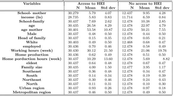
extracting information about her. This sample has the following distribution of those who attended
or did not attend higher education for each year, shown in Table 1.
Table 1: Participants versus non-participants in HEI
Variables Access to HEI No access to HEI
N Mean Std dev N Mean Std dev
School- mother 30.279 5.79 4.07 12.437 9.95 4.28
income (ln) 28.735 5.83 0.83 11.714 6.59 0.84
School-family 30.437 7.69 2.62 12.478 10.38 2.85
age 30.435 26.58 8.29 12.478 22.97 4.79
age mother 30.401 53.58 10.87 12.470 50.21 7.55
Male 30.437 0.48 0.50 12.478 0.44 0.50
Head of family 30.437 0.15 0.35 12.478 0.05 0.21
White 30.403 0.49 0.50 12.468 0.68 0.47
employed 30.436 0.70 0.46 12.478 0.58 0.49
Working hours (week) 30.430 30.12 21.50 12.478 21.06 19.76
Home production 30.436 0.62 0.49 12.478 0.51 0.50
Home porduction hours (week) 30.437 10.29 13.60 12.478 5.69 8.82
eldest 30.437 0.64 0.48 12.478 0.67 0.47
Family size 30.435 4.00 1.50 12.477 3.95 1.17
Southeast 30.437 0.36 0.48 12.478 0.34 0.47
South 30.437 0.14 0.34 12.478 0.19 0.39
Northeast 30.437 0.30 0.46 12.478 0.24 0.43
North 30.437 0.11 0.31 12.478 0.10 0.30
Urban region 30.437 0.93 0.26 12.478 0.97 0.18
Metropolitan region 30.437 0.46 0.50 12.478 0.49 0.50
First, note that there seems to be segmentation in the population between those who continue
into higher education, whether public or private, and those who stop at high school. This
segmenta-tion is also observed in the differences between the (average of) covariates, which are all significantly
different from 0, suggesting that individuals face different restrictions on access to higher education.
Differences between the groups can be seen: average per-capita family income, mothers years of
education, and average years of study for the family weighted by age are much lower among those
who did not attend higher education than those who did. In addition, attending higher education
has positive correlations with being the eldest in the family and being white and negative
correla-tions with being the head of the family, working (in the reference week), and performing household
duties. Table 2 compares the sample of individuals attending public and private HEIs. The average
per-capita family income is larger for those attending private HEIs, but the mothers and familys
education levels are higher for those in the public sector. This result suggests that, once individuals
can attend higher education, income might not be the variable that sorts individuals between public
and private schools. Statistically significant differences are found only between working hours at
home (individuals at private HEIs work more) and whether individuals live in urban areas (also in
Table 2: Participants in public versus participants in private HEI
Private HEI Public HEI
N Mean Std dev N Mean Std dev
School-mother 8.989 9.86 04.26 3 .446 10.2 4 .34
School-mother (sqr) 8.989 115.39 76.51 3 .446 122.78 7 8.16
income (ln) 8.422 6.65 00.81 3 .290 6.44 0 .92
School-family 9.016 10.34 02.82 3 .460 10.49 2 .9
age 9.016 23.18 04.94 3 .460 22.42 4 .31
age (sqr) 9.016 561.86 282.45 3 .460 521.32 2 43.45
age-mother 9.009 50.41 7.67 3 .459 49.67 7 .21
Male 9.016 0.43 0.5 3 .460 0.47 0 .5
Head of family 9.016 0.05 0.22 3 .460 0.04 0 .19
White 9.006 0.7 0.46 3 .460 0.62 0 .49
employed 9.016 0.63 0.48 3 .460 0.47 0 .5
Working hours (week) 9.016 23.3 19.77 3 .460 15.2 1 8.52
Home production hours (week)* 9.016 5.69 8.82 3 .460 5.68 8 .8
eldest 9.016 0.68 0.47 3 .460 0.64 0 .48
Family size 9.015 3.9 1.14 3 . 460 4.08 1 .23
Southeast 9.016 0.38 0.49 3 .460 0.24 0 .43
South 9.016 0.21 0.4 3 .460 0.15 0 .36
Northeast 9.016 0.2 0.4 3 .460 0.35 0 .48
North 9.016 0.08 0.27 3 .460 0.15 0 .36
Urban region** 9.016 0.97 0.18 3 .460 0.96 0 .19
Metropolitan region 9.016 0.51 0.5 3 .460 0.44 0 .5
(*) 1% ; (**) 5% significance tests.
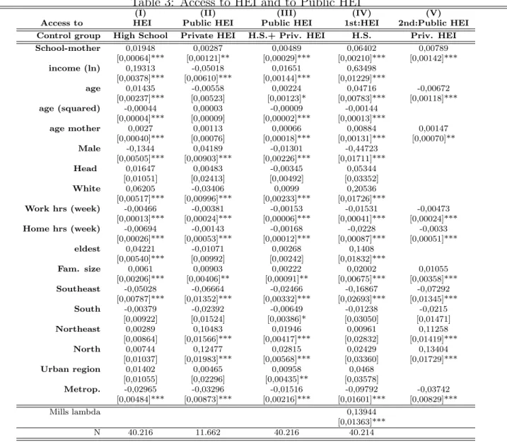
Table 3 summarizes the probabilities of accessing higher education and public HEIs. The results
confirm the positive association of the probability of attending higher education with the mothers
schooling and familys percapita income. We estimate that 1 additional year of mothers education
in-creases the students probability of entering higher education by 1,95p.p.. As well, the determinants
of attending public or private institutions for those already enrolled in higher education are shown in
column (II). We find significant but very low, negative coefficients for per-capita family income and
significant, positive coefficients for mothers schooling. The individuals who access public education
are divided into two groups: those who consume the publicly provided good and those who do not
and could either be in the private sector or not attending higher education at all. A dummy variable
that assigns 1 to the first group and 0 otherwise was built. The results are in column (III). These
results indicate a more direct indicator of the population that consumes publicly provided
educa-tion compared to that those that do not. The signs of the coefficients match the previous findings,
except for the log of per-capita income: in this case, the higher an individuals income is, the more
likely the individual is to have access to public education. From this perspective, individuals with
access to public HEIs in Brazil have better conditions, including family background, compared to
those who attend higher education and those that do not, one must take into account the eventual
selection bias of those groups. Some individuals might be willing to attend higher education, even
if offered by the public sector, but cannot mainly due to existing barriers to access. To correct
for this eventual sample selection bias problem, Heckmans (1977) two-stage procedure is used. In
the first stage, the probability that an individual is eligible for higher education, given a set of
explanatory variables, is calculated. In the second stage, the coefficients of the determining factors
for the chosen higher-education system are estimated, incorporating the inverse Mills ratio, , which
is the ratio of the probability density function and the cumulative distribution function. To correct
possible sample selectivity, at least one explanatory variable with a significant coefficient in the
selection equation is needed as an instrument. When controlling only for age2, other significant
variables to explain the probability of entering higher education are found, but none provides a
significant explanation of enrolling in public schools (dummies for gender, head of family, eldest,
firstborn, urban area, and logarithm of per-capita family income). These are used as identifying
variables in the first stage. Columns (IV) and (V) in Table 2 summarize the results obtained when
correcting for selection bias. The coefficient of the inverse Mills ratio, λ, is significant; therefore,
there was selection bias before the correction.
The results of the first stage are consistent with those of probit previously obtained (Table 2, column (I)). Mothers education level, log of per-capita family income, white race, eldest in the
family, and living in urban areas increase the probability of entering higher education. Notably,
one additional unit of the log of per-capita income raises the likelihood of attending college by
63p.p. These results are in line with expectations and reflect the existing restrictions on access to
higher education in Brazil, where the poorest with the least amount of human capital, for which
mothers education is used as a proxy, do not have easy access to higher education. In the second
stage that explains access to public universities (column (V), Table 2), the main variable is the
mothers education, and the results show that one more year of education increases the students
chance of attending a public HEI by almost 1 p.p. Per-capita income does not have significant
influence on access to public HEI, unlike the significant, negative results observed in column (II).
Therefore, these findings suggest a lack of evidence for income redistribution through the public
Table 3: Access to HEI and to Public HEI
(I) (II) (III) (IV) (V)
Access to HEI Public HEI Public HEI 1st:HEI 2nd:Public HEI
Control group High School Private HEI H.S.+ Priv. HEI H.S. Priv. HEI
School-mother 0,01948 0,00287 0,00489 0,06402 0,00789
[0,00064]*** [0,00121]** [0,00029]*** [0,00210]*** [0,00142]***
income (ln) 0,19313 -0,05018 0,01651 0,63498
[0,00378]*** [0,00610]*** [0,00144]*** [0,01229]***
age 0,01435 -0,00558 0,00224 0,04716 -0,00672 [0,00237]*** [0,00523] [0,00123]* [0,00783]*** [0,00118]***
age (squared) -0,00044 0,00003 -0,00009 -0,00144
[0,00004]*** [0,00009] [0,00002]*** [0,00013]***
age mother 0,0027 0,00113 0,00066 0,00884 0,00147
[0,00040]*** [0,00076] [0,00018]*** [0,00131]*** [0,00070]**
Male -0,1344 0,04189 -0,01301 -0,44723 [0,00505]*** [0,00903]*** [0,00226]*** [0,01711]***
Head 0,01647 0,00483 -0,00345 0,05344 [0,01051] [0,02413] [0,00492] [0,03352]
White 0,06205 -0,03406 0,0099 0,20536
[0,00517]*** [0,00996]*** [0,00233]*** [0,01726]***
Work hrs (week) -0,00466 -0,00381 -0,00153 -0,01531 -0,00473
[0,00013]*** [0,00024]*** [0,00006]*** [0,00041]*** [0,00024]***
Home hrs (week) -0,00694 -0,00143 -0,00168 -0,0228 -0,0033
[0,00026]*** [0,00053]*** [0,00012]*** [0,00087]*** [0,00051]***
eldest 0,04221 -0,01071 0,00268 0,1408
[0,00540]*** [0,00992] [0,00242] [0,01832]***
Fam. size 0,0061 0,00903 0,00222 0,02002 0,01055
[0,00206]*** [0,00406]** [0,00091]** [0,00675]*** [0,00358]***
Southeast -0,05028 -0,06664 -0,02466 -0,16867 -0,07292
[0,00787]*** [0,01352]*** [0,00332]*** [0,02693]*** [0,01345]***
South -0,00379 -0,02392 -0,00649 -0,01238 -0,0215
[0,00922] [0,01524] [0,00386]* [0,03050] [0,01471]
Northeast 0,00289 0,10483 0,01946 0,00961 0,11258
[0,00864] [0,01566]*** [0,00417]*** [0,02832] [0,01419]***
North 0,00744 0,12477 0,02815 0,02429 0,13404
[0,01037] [0,01983]*** [0,00568]*** [0,03360] [0,01729]***
Urban region 0,01402 0,00465 0,00958 0,0468
[0,01055] [0,02296] [0,00435]** [0,03578]
Metrop. -0,02965 -0,03296 -0,01516 -0,09792 -0,03742
[0,00484]*** [0,00873]*** [0,00216]*** [0,01601]*** [0,00829]***
Mills lambda 0,13944
[0,01363]*** N 40.216 11.662 40.216 40.214
the decision whether to invest in higher education and, second, selecting between public or private
HEIsthe first stage seems to be affected by individuals family backgrounds. Families in which the
mothers obtained more advanced schooling tend to value education more, and their children attain
higher public education. Thus, individuals whose mothers have fewer study opportunities might
have lower chances to continue studying and more difficulty accessing public HEIs due to either
the limited number of slots or the availability of more immediately profitable opportunities than
investing in education.
3
Empirical Estimation of HEIs Quality
The aim of this section is to investigate how much Brazilian HEIs add to students knowledge
of field-specific contents. Next, private and public institutions are compared using a panel of
undergraduates, with data from field-specific ENADE tests taken by students early in their studies
(freshman year) and again three years later. The methodology used to estimate such the differences
between higher education systems is explained, followed by an analysis of the databases and results.
3.1
Empirical Method
A study aim is to analyze the difference in the quality of higher education provided by the public
and private sectors using field-specific test data from ENADE for the years 2004 and 2007. The
purpose of this test is to assess the contents for the degree program undergraduates are studying.
Students take the exam twice. The first time, they are considered newcomers and cannot have
completed more than 20% of the curriculum. Three years later, students are considered those who
have finished, having completed at least 80% of the course curriculum. The ENADE, according to
INEP, was designed for assessing student performance in relation to the program content provided
in the curriculum guidelines for undergraduate courses, skills development and the skills necessary
to deepen the general education and training and the level of upgrade of students in relation to
the Brazilian reality and world.3Thus, the difference between students scores on this test evaluating
field-specific content obtained at the end of the program and as newcomers should represent, to
3
some extent, how students have learned during their studies. This learning process can depend on
various factors, such as student effort, ease of learning, and faculty and institution characteristics.
This research is aimed at determining how much of individual knowledge aggregation is due to the
school system and how much to the HEI attended. That is, the aim is to compare the aggregate
knowledge of public and private HEI students, taking into account the effect of other characteristics.
The available database allows comparing individual students when they start and finish programs.
Thus, the intrinsic (non-observable) characteristics of students which do not change over time, such
as effort and skill, are already considered. However, it still needs to be determined how students
compare the two systems and whether the provided selection tests for admission to HEIs create a
self-selection bias between networks. To minimize this bias, a combination of methods is adopted
to maintain comparisons between only students with similar characteristics. The question to be
answered is whether a student in a public HEI would have acquired additional knowledge had the
student attended the same course with same infrastructure and faculty at a private institution.
Thus, it is necessary to find counterparts as close as possible for students in public and private
institutions, that is, students with the same probability of being in a public HEI. First, a probit
model is estimated to identify the probability of attending a public HEI (propensity score P (X)) for
all students with available information on the observable, weighted variables that can affect school
system selection. The underlying assumption is that these variables determine the probability
that a student attends a public HEI instead of a private HEI. The variable of interest is i, the
differential between the two scores of student i (as a newcomer and as those who have finished )
on the objective, field-specific component, i.e., the aggregate of the students knowledge about the
course content learned over three years:
∆(y)i =yi,f inal−yi,initial (1)
where i,j is the field-specific grade for student i in year j. A linear model proposed by Hirano
and Imbens (2001) can be adapted for the present case:
where Zi is a factor characteristic of the HEI the student attends. The fourth term is the
devi-ation of this vector relative to the sample mean ¯Z in the subsample of individuals from public
HEIs, which interacts with the dummy variable of administrative responsibility for the HEI. These
terms are included because these variables related to HEI are characteristics of the faculty and
available infrastructure and could affect students learning process.4 The coefficient τ represents
the parameters of interest of this study: how much of ∆(y)i is due to a student attending a public
HEEs. The advantage of these mixed methods, combining regression and weighting based on the
propensity score, is that it makes the estimator of interest less sensitive to isolated cases of the
two methods, including the selection observed. The estimated effect is doubly robust, removing the
correlation among the variables omitted and reducing the correlation between the variables included
and omitted (Imbens and Wooldridge, 2009; Hirano and Inbems, 2001; Robins and Rotnizky, 1995).
3.2
Data
To investigate the differential of the aggregate knowledge acquired by students in the two higher
education systems, ENADE examination results are used. Following classical theory, a panel of
students is studied, using data from the field-specific, objective component of ENADE administered
to the same learners at the beginning and end of their programs. The objective of ENADE is to
measure how much knowledge college adds students and to measure the quality of institutions by
the difference in the scores of graduates and first-year students. This research compares how much
knowledge public HEIs add to students over the course of their program compared to private HEIs.
Data from the Higher Education Census on HEIs and the programs of study which students join are
also used. The information extracted from these databases also serves as the control variables for
the HEI and students program to determine the effect of aggregate scores on enrolling in a public
HEI, independent of the appropriations of the institution. The INEP started administering the
ENADE annually in 2004 as a replacement for the National Course Exam. For the years studied,
ENADE was conducted with a sample of students in selected courses of study, which varied over
4
the years. Participation in the examination is required for graduation. Test scores from 2004 and
2007 are selected because they allow setting up a panel of students who took the test in 2004 as
newcomers and in 2007 as graduates of the undergraduate programs. The following areas were
evaluated in both years: agronomy, physical education, nursing, pharmacy, physiotherapy, speech
therapy, medicine, veterinary medicine, nutrition, dentistry, social work, occupational therapy, and
animal science. Each student takes four tests: a general exam with objective questions, a general
exam with discursive questions, a field-specific objective exam, and a field-specific discursive exam.
The field-specific components vary depending on students course of study, while the general exams
are the same for all students. In this section, only scores from the field-specific exam with objective
questions answered on a 0100 scale are compared to determine how much expertise in the intended
career for graduates of a course students have learned. The field-specific discursive exam is not used
because many students choose to leave this exam blank, limiting the sample. Thus, the effect of a
degree obtained at a public HEI on the (value) added to students scores in the specific-component
exam is estimated.5 The following student-level information gathered using ENADE is considered:
(i) score on the field-specific exam as a newcomer (2004); (ii) score on the field-specific exam as a
senior (2007); (iii) score on the objective component of the general exam as newcomer (2004); (iv)
student characteristics (gender, race, age); and (v) family characteristics (family income, mothers
education, attended a public high school). Regarding HEIs, the Higher Education Census provides
the following information: (i) faculty characteristics (proportion of professors with doctorates, of
full-time staff, of male teachers, and of professors dedicating at least 70 % of the workload to
research); (ii) infrastructure characteristics (library, proportion of computers with Internet access);
(iii) general characteristics of the course of study (awards bachelor degree, proportion of students
in day and night classes, proportion of students with scholarships covering at least 70 % of tuition
and fees); and (iv) dummies for the Brasilia state and whether the course is held in a state capital.
Therefore, the following variables that could determine the probability of that a student has access
to the public higher education system are studied: scores for the general and field-specific objective
5
Specifically, ∆yi,j=yi,2007−yi,2004is considered, whereyi,jcorresponds to the score obtained on the field-specific
exams as newcomers (grade-go, grade-sc); gender; dummy for black individuals; dummy for low
family income; dummy for high-school educated mother (at least secondary education ); school
system in which the student attended high school (dummy for public high school system); age
when the student enrolled in higher education; and a group of variables that capture the course of
study from the student is graduated. It is assumed that these variables determine the likelihood
of a student being in a public HEI instead of a private HEI. The information provides objective
evidence for matching students with similar intrinsic characteristics. If two students, i and j, one in
a public HEI and one in a private HEI, both obtain similar grades when they are admitted to the
higher education system, in addition to having other similar variables in the propensity score model,
they will have the same probability of being in a public HEI. If the HEI has similar characteristics
(e.g., infrastructure, faculty), any difference in these two students added score over the three years
can be attributed to attending a public HEI instead of a private HEI. Variables that could affect
the (value) added score but not the probability of being in a public HEI are considered: proportion
of professors with doctorates; proportion of professors with exclusive dedication to that HEI; a
dummy indicating the presence of a library on campus; proportion of on-campus computers with
Internet access; offering of an international baccalaureate course; proportion of students attending
day classes; and proportion of students with scholarships covering at least 70% of tuition and fees.
The population of interest in this study is limited to students in either public or private HEIs,
so we ignore the selection bias in access to the higher education system. However, within the
population of interest, there might be another type of selection because various restrictions had to
be imposed on the sample due to database limitations. Some institutions do not require students
to take the exam, so that there is no information on their scores. Nevertheless, we understand that,
on average, this selection does not change the characteristics of the two groups of students from
public and private HEIs. Table 4 shows the mean difference of the value-added scores (∆) and
the number of observations in each school system for different sub-samples: a) all 2004 first-year
students with 2007 scores as graduates; b) only students with ENADE exam scores in both years;
c) those in sample b whom completed the socioeconomic questionnaire; and d) those in sample of
the previous item matched by propensity score.
Table 4: Mean and standard deviation for (value) value-added specific-component exam - ENADE, 2004 - 2007
Variables Private Public Total
N Mean Std. Dev N Mean Std. Dev N Mean Std. Dev a) Full Sample 21.022 0.23 2 7.86 3.752 0.91 33.22 24.774 0.34 28.74
b) + ENADE 8.800 12.20 1 7.90 1.387 16.23 18.58 10.187 12.75 18.05
c) + socioec. 5.982 13.46 1 7.84 912 16.88 18.56 6.894 13.91 17.98
d) + matched 5.865 13.48 1 7.87 886 16.75 18.71 6.751 13.91 18.01
random answers, the average aggregate score rises substantially for both school systems. In samples
(b), (c), and (d), the aggregate score of public school students is statistically higher than that of
private HEI students. It is noteworthy that, despite the proportional reduction in the sample size
from sample (a) to sample (d), the two samples seem similar between the HEI types (72.1 % in
private and 76.4 % in public). The proportional increase in average score is higher among students
at private HEIs than public HEIs (58 times increase in the average score of private HEIs and 18
times the average score of public HEIs). This result indicates that, with the restriction of the
sample, the students at private HEIs become more selective than students at public HEIs. Sample
(d) is used in the estimations, and Table 7 shows the average differences of the propensity score
and the variables used in the regression analysis among school systems.
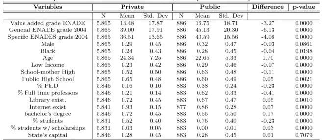
Table 5: Descriptive statistics - Restricted sample of public versus private HEI’ students
Variables Private Public Difference p-value
N Mean Std. Dev N Mean Std. Dev
Value added grade ENADE 5.865 13.48 17.87 886 16.75 18.71 -3.27 0.0000 General ENADE grade 2004 5.865 39.00 17.91 886 45.13 20.30 -6.13 0.0000 Specific ENADES grade 2004 5.865 36.51 13.65 886 40.59 15.56 -4.08 0.0000 Male 5.865 0.29 0.45 886 0.32 0.47 -0.03 0.0861 Black 5.865 0.24 0.43 886 0.28 0.45 -0.04 0.0198 Age 5.865 24.34 7.25 886 22.65 5.33 1.70 0.0000 Low Income 5.865 0.23 0.42 886 0.29 0.46 -0.07 0.0000 School-mother High 5.865 0.52 0.50 886 0.63 0.48 -0.11 0.0000 Public High School 5.865 0.65 0.48 886 0.60 0.49 0.05 0.0021 % Ph.D 5.846 0.16 0.10 883 0.38 0.24 -0.23 0.0000 % Full time professors 5.846 0.21 0.14 883 0.62 0.33 -0.41 0.0000 Library exist. 5.846 0.72 0.45 883 0.67 0.47 0.05 0.0010 Internet exist 5.841 0.93 0.15 877 0.86 0.28 0.07 0.0000 bachelor’s degree 5.846 0.72 0.45 883 0.55 0.50 0.17 0.0000 % students 5.831 0.52 0.40 883 0.75 0.40 -0.23 0.0000 % students w/ scholarships 5.831 0.03 0.05 883 0.00 0.01 0.03 0.0000 State’s capital 5.846 0.28 0.45 883 0.28 0.45 0.01 0.7079
Most group variables show significant difference. For example, among the variables related to
family characteristics, the average education level of mothers and the proportion of students who did
The highest proportions of Ph.D. holders and professors exclusively dedicated to a single institution
are at public institutions. Students attending day classes are also more numerous at public HEIs.
However, students of private institutions have more access to computers than students at public
HEIs. In private HEIs, the dropout rate throughout the course for the analyzed sample is much
higher than in public HEIs. For the variable of interest, the difference in the aggregate scores for
the field-specific objective component is significant and higher among students at public HEI.
3.3
Results
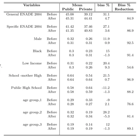
The non-balancing problem between the two groups can be corrected using the propensity score
method. Table 8 shows the percentage reduction in the standard bias (SB) for each variable used
in the propensity score. The standard percentage bias is the percentage difference between the
average of the treated (attending public HEI) and untreated samples (attending private HEI) as a
proportion of the square root of the sample means variance in both groups (Rosenbaum and Rubin,
1985). 6
Note that, before being matched based on propensity score, private and public HEI students have
different averages on all variables. Therefore, making comparisons between these two groups could
not be reliable. After balancing, one might consider groups of students at different institutions with
similar characteristics, taking into account their estimated probability of attending a public HEI. In
addition, common support for the estimated propensity score is found: all students are considered
within the support; that is, no value of the propensity score is associated with a specific group. 8
Table 7 shows the results of the probit estimation, including the marginal effects. The estimated
probability that a student is enrolled in the public system based on the students characteristics is
used to re-weight the sample:
The results show that a highly educated mother increases by 3,4p.p. the probability of a student
attending a public HEI, and having attended a public high school during basic education reduces
6
Specifically,SB= (100∗((xpriv)−(xpub)))/(((s2
priv+s
2
pub))/2).
8
Table 6: Covariates before and after matching and bias reduction
7.
Variables Mean bias % Bias %
Public Private Reduction
General ENADE 2004 Before 45.08 39.12 31.1
After 45.31 44.41 4.7 84.9
Specific ENADE 2004 Before 41.42 37.46 27.1
After 41.35 40.83 3.6 86.9
Male Before 0.32 0.26 11.9
After 0.31 0.31 0.9 92.5
Black Before 0.3 0.23 15
After 0.3 0.31 -1.3 91.4
Low Income Before 0.31 0.22 20.4
After 0.3 0.26 9.3 54.6
School -mother High Before 0.64 0.54 21.5
After 0.64 0.64 0.7 96.9
Public High School Before 0.58 0.64 -11.2
After 0.58 0.59 -1.3 88.2
age group 1 Before 0.29 0.33 -9
After 0.28 0.27 2.1 76.6
age group 2 Before 0.32 0.19 28.2
After 0.32 0.34 -5.3 81.4
age group 3 Before 0.19 0.14 12
After 0.19 0.19 -1.3 89.1
Table 7: Probability of access to Public HEI
Variables Public HEI
General ENADE 2004 0,00164 [0,00019]*** Specific ENADE 2004 0,00204 [0,00026]*** Male -0,01319 [0,00791]* Black 0,05103 [0,00881]*** Low Income 0,06191 [0,00946]*** School-mother High 0,03391 [0,00758]*** Public High School -0,01494 [0,00793]* age group 1 0,03905 [0,01093]*** age group 2 0,12058 [0,01361]*** age group 3 0,07688 [0,01385]*** R2 Pseudo 0,09 Log likelihood -3.285,04
N 9.188
that probability.9 If the student claims to be black and declares a low family income, the likelihood
of attending a public HEI. The effect of the HEIs education network on aggregate score, where the
treatment is public higher education, calculated by matching based on propensity score, indicates a
difference of 3.83 points in the aggregate scores of students at public and private HEIs, statistically
different from 0. That is, considering the balanced sample, public HEI students have a higher
aggregate score than private HEI students. However, when applying the reweighting method, the
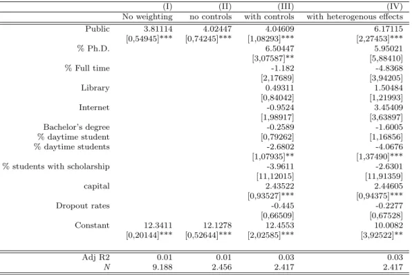
obtained effect of the HEIs education system on aggregate scores is higher. Table 10 shows the
results of the regressions of the aggregate scores on the field-specific, objective component to different
specifications. Column (I) presents the results of the estimation without using the propensity
score estimated as a weight to the observations. This estimation considers the unbalanced sample,
without taking into account the probability of pupils being in a public HEI instead of the private
given their characteristics. This group has an aggregate score difference of 3.81. When considering
the estimated probability as a weight in the regression, as in column (II) of Table 10, the effect
of attending a public HEI on aggregate student scores rises to 4.02 points. However, in this case,
the characteristics of the faculty and the institutions infrastructure are not believed to have specific
effects on aggregate scores, and any effects of these variables should be captured by the coefficient of
the educational system. These control variables of HEI are included in column (III), so the coefficient
of interest represents only the effect of the educational system, net of the other characteristics of
the HEI. The effect becomes slightly larger, 4.05, and remains significant at 1 %. The proportion
of professors with doctorates in the faculty increases the aggregate student score by 6.50 points.
Finally, column (IV) allows for heterogeneous effects from the variables between the groups of
students and the characteristics of the institutions. In this specification, the effect of school system
on aggregate index increases to 6.17 points.
These estimates indicate that, regardless of the method used, the school system of the students
HEI has a significant effect on the aggregate score of field-specific exam component. In other
words, public HEI students have a higher aggregation value of scores than students at private HEIs.
There are indications that the quality offered by undergraduate public institutions is superior to
that offered by the private higher-education system. If students observe this difference in quality
9
Table 8: Specific ENADE score, weighted by the propensity score
(I) (II) (III) (IV) No weighting no controls with controls with heterogenous effects Public 3.81114 4.02447 4.04609 6.17115 [0,54945]*** [0,74245]*** [1,08293]*** [2,27453]***
% Ph.D. 6.50447 5.95021
[3,07587]** [5,88410]
% Full time -1.182 -4.8368
[2,17689] [3,94205]
Library 0.49311 1.50484
[0,84042] [1,21993]
Internet -0.9524 3.45409
[1,98917] [3,63897] Bachelor’s degree -0.2589 -1.6005 % daytime student [0,79262] [1,16856] % daytime students -2.6802 -4.0676 [1,07935]** [1,37490]*** % students with scholarship -3.9611 -2.6301 [11,12015] [11,91359]
capital 2.43522 2.44605
[0,93527]*** [0,94375]*** Dropout rates -0.445 -0.2277 [0,66509] [0,67528] Constant 12.3411 12.1278 12.4553 10.0082 [0,20144]*** [0,52644]*** [2,02585]*** [3,92522]**
Adj R2 0.01 0.01 0.03 0.03
N 9.188 2.456 2.417 2.417 ∗p <0,1;∗ ∗p <0,05;∗ ∗ ∗p <0,01.Note: Standard error in parenthesis.
Control group weighted less than one for Private institutions’ students.
indicated by these results, it could influence their preferences for a particular HEI. Andrade et al
(2009) present evidence that among the characteristics of HEIs that can influence demand among
students is the average ENADE score of admitted students. These factors can increase competition
for public HEI slots, resulting in segmentation between the groups of students who can and cannot
gain these places.
4
Decomposition of freshmans grades differential
Next, the grade differential of first-year students in higher education is decomposed into the objective
portion of the high school exam (ENEM) and the general exam (ENADE). The aim of these tests
is to assess students general knowledge and reading comprehension ability. Students results are
influenced not only by their former school life but also by their family environment, effort, and
intrinsic ability. The effect of each observable factor is broken down, and the decomposition of
students for both HEI systems is compared. To decompose the grade differential between public
permits considering the observable characteristics of one group (treated: public HEI) to build
contrafactuals to other group (untreated: private HEI). Note that a casual interpretation is not
possible, but a correlation between observable factors and grade differentials is. Following Fortin,
Lemieux, and Firpo (2010), it is assumed in the estimation of this decomposition that the target
variable is linearly related to the covariates, so each group is estimated using the following equation,
in which the error term is also assumed to be conditionally X independently :
Ygi =βg0+
K
X
k=1
[Xikβgk] +vgi (3)
where g=A,B represents the two groups (public and private HEI), E(vgi|Xi) = 0, and X is the
covariate vector Xi = [Xi1, , XiK]. The total differential of these scores is calculated as:
c
∆µO =YcB−YcA (4)
c
∆µO= [βdB0−dβA0] +
K
X
k=1
XBk[βdBk−dβAk+ K
X
k=1
][βdAk][XBk−XAk] (5)
The last term of this total differential is the effect of quantity, here called the explained part
of the decomposition. This part refers to the different allocations of the two groups. The score
difference between students enrolled in public and private institutions can be partially attributed
to public-sector students possession of more favorable characteristics for achieving higher scores.
The first two terms constitute the unexplained part of the decomposition. Here, in addition to
the differences between the individual regressions, the constants of the groups are a measure of the
difference between the estimated coefficients of the covariates for sample B compared to sample A.
Thus, by estimating the difference between the scores of the two groups of students, this unexplained
part, assuming that there are no unobservable explanatory variables relevant to it, can be attributed
to the covariates different return. Thus, for example, students in the different groups might have
different returns from their family background or university infrastructure. In this case, students are
divided among institutions with different administrative categories, so the aim of the decomposition
is to explain whether there are significant differences between these two populations. If the explained
have better initial allocations of the observed characteristics. However, if a significant portion of
the total differential is attributable to the unexplained part, then students in public HEI can earn
higher returns on these characteristics than students at private HEIs. These differences can support
the inference that segregation exists between these groups as public universities select students with
higher human capital endowments than their counterparts enrolled in private HEIs. Several studies
have investigated the differences in scores obtained by two mutually exclusive groups of students
distinguished by, for example, gender (Sohn, 2008), while others have investigated the differences
between countries (MCEWAN and Marshall 2004) and schools (Krieg and Storer, 2006). Krieg and
Storer (2006), for example, compare schools in the United States which achieved and failed to achieve
progress goals. The purpose of their study is to determine the extent to which school characteristics
are crucial and to what extent students grades are determined by individual characteristics and
student groups. Krieg and Storer (2006)find that much of the difference between schools that
achieved the proposed goals and those that did not is explained by students characteristics but not
by the factors controlled by school administrators.10
4.1
Data
To investigate the differential in scores obtained by students entering higher education, the ENADE
survey (actual year) and ENEM (the previous year) are used. The latter serves as a measure of
students ex-ante capacity. This assessment determines to what extent there is a selection of those
with better socioeconomic conditions or school performance which could result in access to highly
ranked public institutions. The objective is to assess students human capital endowments before
choosing between public and private universities and then to limit the population of interest to those
students. The sample is also restricted to students who took the ENEM exam in the year before
they entered higher education. Students scores on the ENEM and average scores in high school are
collected. The latter are used as a proxy for the quality of their education before entering higher
education. Higher Education Census information about HEIs and programs of study are enrolled
are also used. Thus, it is possible to determine whether the grade differential between students in
10
public and private schools can be explained by differences in institutional characteristics, such as
physical infrastructure and faculty. The population of interest is restricted to incoming students,
so it is assumed that the university has not yet intervened in students formation of human
cap-ital. Effects related to the institution and the course of study that might affect students scores
are attributable to possible peer-effects; in other words, students benefit from better institutional
characteristics by participating in the group. For the years analyzed, the ENADE exam was still
administered to a sample of students in selected programs that vary by year. We consider the
years 2005 and 2006 because the availability of the data. With ENADE for this period we can
connect students using their identification number to the ENEM data (2004 and 2005).11 In 2005,
the following fields were evaluated: architecture and urbanism, biology, social sciences, computing,
engineering (eight groups), philosophy, physics, geography, history, literature, mathematics,
educa-tion, and chemistry. In 2006, the programs evaluated were business administraeduca-tion, archival and
library science, biomedicine, accounting, economics, media, design, law, teacher training (normal
superior), music, psychology, executive secretary, theatre, and tourism. Only scores on the
objec-tive, general-education exam are compared, so the possibility of bias on the type of test (discursive
grading) and field exam can be excluded. Also excluded are students who left their test or
socioe-conomic questionnaire blank (therefore a null score) or responded in a random fashion, namely,
choosing the same option for all questions. The following information categories are extracted from
ENADE: (i) personal characteristics (gender, race, age, speaks English or Spanish, reads books
other than academic texts, uses computers); (ii) family characteristics (marital status, number of
children, head of the family, family income, mothers and fathers education, attendance at a public
or private high school, studying at a regular or technical high school); (iii) academic characteristics
(morning or night classes, educational funding); (iv) academic effort (weekly hours dedicated to
studying, performing research activities or other activities at the HEI, uses of the HEI library);
(v) HEI characteristics (proportion of professors with doctorates, of full- and part-time lecturers,
of research-oriented professors, of male professors, and of computers with Internet access); and
(vi) infrastructure characteristics (presence of a library, proportion of students with a scholarship
covering at least 70% of tuition and fees). In addition, dummies are included for year, Brazilian
11
region, state of residence, and whether a program is held in a state capital. Notably, the population
of interest in this study is limited to students at public and private HEIs, so the selection bias due
to access to the university is ignored, unlike in section 3. 12. Note that we are interested in the
objective portion of ENEM taken the year before entering university and the score on objective
general-education portion of ENADE in the years 2005 and 2006. Both these scores answered on
a scale of 0100 are extracted from INEP and standardized. 13 Table 9 shows the mean absolute
standards and the number of scores and observations for each education network in different types
of samples: a) all 2005 and 2006 entrants ; b) first-year students able to take general ENADE exam;
c) students in the previous item who completed the socioeconomic questionnaire ; d) students in
the previous item who took the ENEM test in the previous year; and e) those in the previous item
with available information on where they attended high school.
Table 9: Freshman’s grade on general exam ENADE(2005-2006) and ENEM(2004)
Variable Private HEI Public HEI
N Mean Std dev. N Mean Std dev.
(a) All freshman 244,991 46.26 -0.06 88.871 52.71 0.16
(b) + proper ENADE 179,201 55.70 0.26 60.545 66.86 0.63
(c)+ socioeconomic 144,575 55.38 0.25 44.977 66.52 0.62
(d)+ ENEM 28.708 52.86 0.16 5.999 65.34 0.58
(e)+ Scholar Census
Enade’s grade 17.114 53.75 -0.02 3.676 64.98 0.46 Enem’s grade 17.114 47.62 -0.04 3.676 59.83 0.56
The average ENADE score is higher in sample (b) than sample (a) because the former excludes
those who answered items improperly or boycotted the exam. One can see that the average ENEM
score is lower than ENADE scores overall. However, the differences between students at public and
private HEIs remain significant. Accordingly, the sample in Table 10 is limited to students who
have a valid ENADE assessment, answered the socioeconomic questionnaire, and are found in the
ENEM data. Sample (e) in Table 9 is used in the decomposition of the score differential. The
12
However, within the population of interest, there may be another type of selection because various restrictions are imposed on the sample. Some students boycotted the ENADE tests, so that there is no information on their scores. As well, some scores were not found in ENEM data, often due to record-keeping mistakes. This selection does not seem to change, on average, the characteristics of the two groups (public and private HEIs
13
average differences of the remaining variables are also presented.
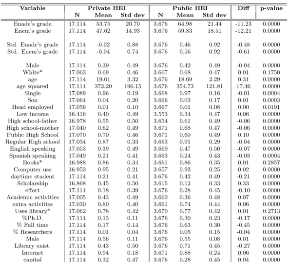
Table 10: Restricted sample with proper information on all datasets
Variable Private HEI Public HEI Diff p-value
N Mean Std dev N Mean Std dev
Enade’s grade 17.114 53.75 20.70 3.676 64.98 21.44 -11.23 0.0000 Enem’s grade 17.114 47.62 14.93 3.676 59.83 18.51 -12.21 0.0000
Std. Enade’s grade 17.114 -0.02 0.88 3.676 0.46 0.92 -0.48 0.0000 Std. Enem’s grade 17.114 -0.04 0.74 3.676 0.56 0.92 -0.61 0.0000
Male 17.114 0.39 0.49 3.676 0.42 0.49 -0.04 0.0000 White* 17.063 0.69 0.46 3.667 0.68 0.47 0.01 0.1750 age 17.114 19.01 3.32 3.676 18.69 2.29 0.31 0.0000 age squared 17.114 372.20 196.15 3.676 354.73 121.81 17.46 0.0000 Single 17.089 0.96 0.19 3.668 0.97 0.16 -0.01 0.0004 Son 17.064 0.04 0.20 3.666 0.03 0.17 0.01 0.0003 Head employed 17.056 0.01 0.10 3.667 0.01 0.08 0.00 0.0191 Low income 16.416 0.40 0.49 3.553 0.34 0.47 0.06 0.0000 High school-father 16.978 0.55 0.50 3.654 0.61 0.49 -0.06 0.0000 High school-mother 17.040 0.62 0.49 3.671 0.68 0.47 -0.06 0.0000 Public High School 17.070 0.70 0.46 3.671 0.60 0.49 0.10 0.0000 Regular High school 17.034 0.87 0.33 3.663 0.91 0.29 -0.04 0.0000 English speaking 17.053 0.39 0.49 3.669 0.47 0.50 -0.07 0.0000 Spanish speaking 17.049 0.21 0.41 3.663 0.24 0.43 -0.03 0.0004 Books* 16.988 0.86 0.34 3.661 0.86 0.35 0.01 0.2857 Computer use 16.953 0.95 0.21 3.657 0.93 0.25 0.02 0.0000 daytime student 17.114 0.21 0.41 3.676 0.42 0.49 -0.21 0.0000 Scholarship 16.868 0.45 0.50 3.615 0.12 0.33 0.33 0.0000 effort 17.114 0.18 0.39 3.676 0.28 0.45 -0.10 0.0000 Academic activities 17.005 0.43 0.49 3.660 0.36 0.48 0.07 0.0000 extra activities 17.030 0.80 0.40 3.661 0.74 0.44 0.06 0.0000 Uses library* 17.062 0.78 0.42 3.670 0.77 0.42 0.01 0.2713 %Ph.D. 17.114 0.13 0.11 3.676 0.30 0.23 -0.17 0.0000 % Full time 17.114 0.17 0.14 3.676 0.63 0.30 -0.45 0.0000 % Researchers 17.114 0.01 0.04 3.676 0.05 0.15 -0.04 0.0000 Male 17.114 0.56 0.11 3.676 0.55 0.08 0.01 0.0000 Library exist. 17.114 0.43 0.50 3.676 0.71 0.45 -0.27 0.0000 Internet 17.114 0.94 0.18 3.671 0.88 0.24 0.06 0.0000 capital 17.114 0.32 0.47 3.676 0.28 0.45 0.04 0.0000
Variables with (*) are not statically different between private and public HEIs.
In Table 10, it can be seen that most variables are statistically different between groups. Only the
proportion of whites, the average number of extracurricular books read, and the proportion of HEI
students using the library to study are equivalent between the two groups. For all other variables,
significant differences are found on average. Among the variables related to family characteristics,
for example, public HEI students have higher average family income, fathers and mothers education
level, and proportion of students who have not studied in a public school high school system but
attended a regular high school. The variables related to institutions faculty are also as expected:
public HEIs have the largest proportion of Ph.D. holders, exclusively dedicated instructors, and
researchers in their faculties. Also more common in public HEIs are students who attend day
out more academic and extracurricular activities and have more computer access on average. More
importantly, the differences in standardized scores on the two exams, ENADE and ENEM, are
significant. Such data provide evidence that public HEIs select students who obtain the best results
in these tests, independent of socioeconomic conditions. The decomposition effects on ENEM and
ENADE scores are separated as follows.
4.2
Decomposing First-Year Students ENADE Scores
The scores obtained by students before they enroll in private and public institutions are compared
to identify their determinants. Students ENEM scores demonstrate how much they learned in high
school and might capture aggregated knowledge from years of study, students stress and innate skills,
and the effects of family background. However, to better compare students skills not observable
to the researcher, more controls for the high schools attended by students are included. Table
11 shows the decomposition results for ENEM scores, where the basis group refers to students at
private HEIs and the score difference refers to public-sector students average score subtracted from
the score of private HEI students. Column (I) shows the decomposition of standardized scores for
the ENEMs objective portions and includes students personal characteristics and family background
as explanatory variables and controls across geographic variables. In column (II), other considered
variables include the average score on the objective portion of ENEM obtained by the high school
where the student attended as a measure of that schools quality.
The decomposition results indicate a difference of−0.61 points in the standardized ENEM scores
of students at private institution and public HEIs. Column (I) shows that the explained portion
of this difference is quite low, −0.10, although significant. Among the variables that contribute to
increasing the score differential between these institutions are family income and parental education.
Due to a lack of more school controls, the unexplained portion of the decomposition may remain
quite high. However, including HEIs average scores, which serve as a synthesis of all the institutions
characteristics (both supply and demand), provide a significant explanation of (-0.19.) the skill
differential between those who attend public and private HEIs. However, the unexplained portion
Table 11: Oaxaca-Blinder decomposition for ENEM
(I) (II)
Private -0,05231 -0,05231 [0,00587]*** [0,00587]*** Public 0,56168 0,56168
[0,01566]*** [0,01565]*** Difference -0,61399 -0,61399
[0,01672]*** [0,01672]***
Variables Explained Unexplained Explained Unexplained
total -0,10126 -0,51273 -0,19238 -0,42161 [0,00979]*** [0,01486]*** [0,01179]*** [0,01355]***
ENEM -0,16526 0,07025 [0,00863]*** [0,06935] Male -0,01033 -0,02462 -0,00977 -0,02142
[0,00242]*** [0,01077]** [0,00229]*** [0,00996]** White 0,00036 -0,00432 0,0001 -0,00808
[0,00039] [0,01915] [0,00014] [0,01773] Age -0,015 -0,02959 -0,0131 0,0974
[0,00367]*** [0,63593] [0,00337]*** [0,58658] Age squared 0,01208 0,07119 0,01108 0,00711
[0,00324]*** [0,23530] [0,00303]*** [0,21695] Male -0,00078 0,10525 -0,0004 0,10349
[0,00049] [0,09376] [0,00044] [0,08661] Son 0,00103 0,00146 0,00115 0,00239
[0,00051]** [0,00257] [0,00051]** [0,00238] Head Employed 0,00072 0 0,00071 0,00024
[0,00035]** [0,00098] [0,00034]** [0,00091] Low income -0,00473 0,06202 -0,00191 0,04356
[0,00101]*** [0,01031]*** [0,00073]*** [0,00960]*** High Schooling father -0,00392 0,00756 -0,00122 0,02485
[0,00096]*** [0,01818] [0,00075] [0,01690] High Schooling mother -0,00257 -0,0114 -0,00078 -0,00899
[0,00089]*** [0,02070] [0,00078] [0,01915] Public High school -0,0277 0,07976 0,01603 0,14536
[0,00275]*** [0,01840]*** [0,00216]*** [0,01939]*** regular High chool -0,00045 -0,05181 -0,00232 -0,05001
[0,00064] [0,04024] [0,00069]*** [0,03722] English speaking -0,01132 0,00255 -0,00707 0,01457
[0,00166]*** [0,01238] [0,00120]*** [0,01156] Spanish speaking 0,00098 0,01346 0,00112 0,00911
[0,00050]** [0,00700]* [0,00049]** [0,00647] Books 0,00024 -0,01455 0,00035 -0,00232
[0,00028] [0,03029] [0,00039] [0,02801] Computer Use 0,00329 -0,08183 0,00325 -0,03219
[0,00092]*** [0,05022] [0,00090]*** [0,04652] Region 0,06446 -0,33125 0,04189 -0,2646
[0,01522]*** [0,16931]* [0,01423]*** [0,15744]* State -0,03314 0,12889 -0,02453 0,08753
[0,01500]** [0,04210]*** [0,01407]* [0,03901]** Capital 0,00475 -0,10788 0,00293 -0,05984
[0,00130]*** [0,00982]*** [0,00085]*** [0,00916]*** year -0,07923 0,00952 -0,04461 0,00719
[0,00400]*** [0,01851] [0,00305]*** [0,01768] Constant -0,33714 -0,58719
[0,46785] [0,43598]
unobservable characteristics might determine the performance gap between institution types. Two
unobserved but relevant variables determining students scores could be their innate ability and
effort exerted. In the following section, it is assumed that the residuals of the regression of the
objective ENEM exam score which are not explained by observable variables (two-thirds of the
ENEM score) are associated with students ability (non-observable characteristic).
4.3
Decomposing First-Year Students ENADE Scores
At the present stage, it is assumed that the ENEM score, net of observable characteristics, is
ap-proximately the same as the students ability because this unobservable characteristic is incorporated
in the residuals. Thus, we use ENEM as an explanatory grade on the decomposition of newcomers
general-education ENADE grades, as proxy to capture the portion of the ENADE score which can
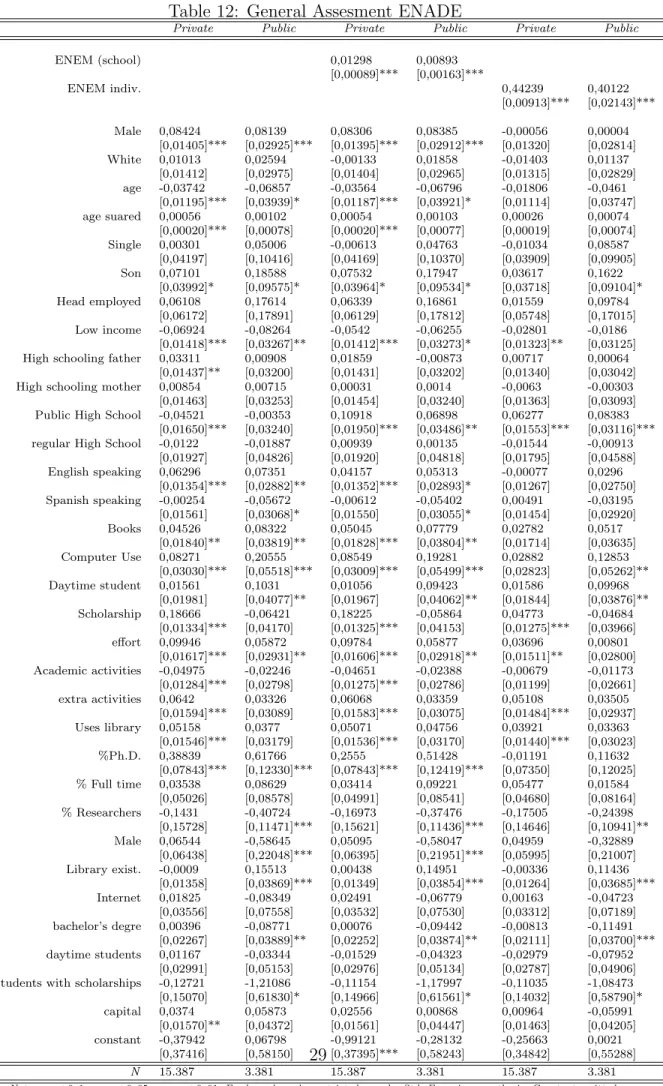
be attributed to skill of the students.14 Table 12 shows the regression results for each group at
three different specifications used to perform the decomposition, in other words, where the
depen-dent variable is the standard score for the objective, general-education component. The sample size
of the students at private HEIs is larger than those at public HEIs. In general, the variables in
both groups act in the same direction, but a larger magnitude for students in the private education
system.15
In the first specification (*columns I and II), a simple model is presented. The model includes
five blocks of variables related to the student (individual characteristics, family, inclusion, academic,
and effort) and three blocks pertaining to the institution and the course of study. In the second
specification (columns III and IV), we include as an explanatory variable of students average of
their high schools ENEM results. Thus, the average ability of students with whom one has studied
is controlled for as a possible proxy of school quality and peer effect before entering college. A
positive, significant coefficient is obtained for this variable, but the coefficient is higher for private
schools than public ones. In other words, the average public school in the ENEM contributes
more to students education than public HEIs. The last model (columns (V and VI) of Table 12
14
It seems reasonable to assume that there is no school-effect on students ENADE scores because the test assesses cognitive skills and knowledge acquired before entering the institution.
15


![Table 11: Oaxaca-Blinder decomposition for ENEM (I) (II) Private -0,05231 -0,05231 [0,00587]*** [0,00587]*** Public 0,56168 0,56168 [0,01566]*** [0,01565]*** Difference -0,61399 -0,61399 [0,01672]*** [0,01672]***](https://thumb-eu.123doks.com/thumbv2/123dok_br/15697580.119086/27.918.203.717.180.1025/table-oaxaca-blinder-decomposition-enem-private-public-difference.webp)