Áxions, májorons e neutrinos em extensões do modelo padrão

(1)

✡✡✡ ✪✪ ✪ ✱✱

✱✱ ✑✑✑ ✟✟ ❡

❡❡ ❅

❅_❅ ❧

❧ ❧ ◗

◗◗ ❍ ❍P P P ❳❳ ❳ ❤❤ ❤ ❤

✭ ✭ ✭

✭✏✟✏

IFT

Instituto de F´ısica Te ´orica Universidade Estadual Paulista

TESE DE DOUTORAMENTO IFT–T.003/2011

´

Axions, M ´

ajorons e Neutrinos em Extens ˜

oes do Modelo

Padr ˜

ao

Bruce Lehmann S ´anchez Vega

Orientador

Prof. Dr. Juan Carlos Montero Garcia

(2)

DEDICATION

Ao Charme da minha vida, Fl ´avia Sobreira S ´anchez.

“I seem to have been only like a small boy playing on the sea-shore, diverting myself in now and then finding a smoother pebble or a prettier shell than the ordinary, whilst the great ocean of truth lay all undiscovered before me”

(3)

ACKNOWLEDGMENTS

It is impossible for me to mention in a small piece of paper, all people whom I will be eternally grateful. Hence, I have decided only to mention those people who are into the deepest of my heart and/or have made this doctoral thesis possible, although this is not the fairest decision.

First of all, I am deeply grateful to my parents and sister who wisely took many decisions which are the responsible for I am here trying to write some fair grateful words. My father, “el careloco” as I lovingly refer to him, has always been involved in the most important decisions in my life. In particular, he has tried desperately to teach me the wise thought of responding to the death with life, to the violence with peace, to the problems with solutions. His smile has been always on my mind, because each one meant a new idea, a new journey which most of the time we never successfully ﬁnished. But, it has been through trial and error that I have learned most of what I know about the life. My mother, Anita, I would like to thank specially to insist in a wonderful fact that, by sharing experiences and lessons learnt, we all learn from each other, to our mutual beneﬁt. My sister, Karina with who grew up, and who always bring happiness to my heart. In conclusion, deep down in my heart, I love you.

Special thanks must go to my dear wife, Fl ávia. I would like to dedicate this thesis to her. Also, I must thank to others not less important people like Juan Mon-tero, my Ph.D. adviser, to Ilya D. Mikhailov, my outstanding bachelor adviser, to my friends: Adriano Sobreira, Alberto Sanoja, Alex Dias, Alexis Roa, Ciro Vega, Cristhian Osório, Débora Sobreira, Elaine Silva, Fabricio Acauhi, Freddy Poveda, Hans Garcia, Humberto Gomez, Jo ão dos Anjos, John Ramirez, Jorge Sobreira, José Vega, Liliane Sobreira, Luis Soriano, Luis Young, Marcelo Guzzo, Marcio Woitek, Marcos Rodriguez, the chessmaster Miguel Vega, Nat ália Sobreira, Pedro S ánchez, Pilar Bonilla, Rogério Rosenfeld, my dear friend Sonia S ánchez, Sttella Sobreira, Vi-cente Pleitez and to the loving memory of Carmen Sofia S ánchez Colmenares.

(4)

RESUMO

Nesta tese, part´ıculas tais como áxions, M ájorons e neutrinos s ão consideradas em duas extensões eletrofracas do modelo padr ão da f´ısica de part´ıculas. Especifi-camente, os modelos considerados est ão baseados nas simetrias de gaugeSU(3)L⊗

U(1)X eSU(2)L⊗U(1)Y′⊗U(1)_B

−L. Primeiramente, no contexto do modelo 3-3-1 com

um sector escalar m´ınimo é realizado um estudo detalhado referente à implementaç ão da simetria de Peccei-Quinn (PQ) para resolver o problema CP forte. Para a vers ão original do modelo, que possui apenas dois tripletos escalares, é mostrado que a Lagrangiana total é invariante sobre uma simetria PQ. No entanto, o áxion n ão é produzido porque um sub-grupo permanece sem quebrar. Embora, neste caso, o pro-blema CP forte possa ser resolvido, a soluç ão é amplamente desfavorecida porque três quarks n ão têm massa em todas as ordens da teoria de perturbaç ão. A adiç ão de um terceiro tripleto escalar resolve o problema dos quarks sem massa, mas o áxion que aparece é vis´ıvel. Para fazer o modelo real´ıstico teremos que modific á-lo. É mostrado que a adiç ão de um singleto escalar junto com uma simetria de gauge discretaZN é

capaz de levar a cabo esta tarefa e proteger o áxion de efeitos da gravidade qu ântica. Para ter segurança que a simetria de gauge discreta que protege o áxion é livre de anomalias, é usada uma vers ão discreta do mecanismo de Green-Schwarz.

A seguir, é considerado um modelo eletrofraco baseado na simetria de gauge SU(2)L⊗U(1)Y′ ⊗U(1)_B₋_L, no qual temos neutrinos de m ão direita com n úmeros

qu ânticos exóticos e diferentes. Devido a esta particular carater´ıstica, é poss´ıvel ter-mos de massa e de Yukawa para os neutrinos, com campos escalares que podem ad-quirir valores esperados do v ácuo (VEVs) pertencendo a escalas de energia diferentes.

´

E feito um estudo detalhado dos setores dos escalares e dos neutrinos para mostrar que o modelo é compat´ıvel simultaneamente com as escalas de massa e a matriz de mistura tribimaximal que s ão inferidas dos dados de neutrinos solares e atmosféricos. Também, é mostrado que o modelo poderia possuir candidatos à matéria escura se uma simetriaZ2 é inclu´ıda.

Finalmente, é discutido uma extens ão supersimétricaN = 1do modeloB₋Lcom três neutrinos de m ão-direita.

Palavras Chaves: ´Axions, M ´ajorons, neutrinos, modelos 3-3-1, modelo B ₋ L, o problema CP forte.

´

(5)

ABSTRACT

In this doctoral thesis axions, Majorons and neutrinos are considered into differ-ent electroweak extensions of the standard model of the particle physics. Speciﬁcally, the two models considered are based on theSU(3)L⊗U(1)X and SU(2)L⊗U(1)Y′ ⊗

U(1)B−Lgauge symmetries. Firstly, in the framework of a 3-3-1 model with a minimal

scalar sector a detailed study concerning the implementation of the PQ symmetry in order to solve the strong CP problem is made. For the original version of the model, with only two scalar triplets, it is shown that the entire Lagrangian is invariant under a PQ-like symmetry but no axion is produced since aU(1) subgroup remains unbroken. Although in this case the strong CP problem can still be solved, the so-lution is largely disfavored since three quark states are left massless to all orders in perturbation theory. The addition of a third scalar triplet removes the massless quark states but the resulting axion is visible. In order to become realistic the model must be extended to account for massive quarks and invisible axion. It is shown that the addition of a scalar singlet together with a ZN discrete gauge symmetry

can successfully accomplish these tasks and protect the axion ﬁeld against quantum gravitational effects. To make sure that the protecting discrete gauge symmetry is anomaly free, a discrete version of the Green-Schwarz mechanism is used.

Secondly, an electroweak model based on the gauge symmetrySU(2)L⊗U(1)Y′ ⊗

U(1)B−Lwhich has right-handed neutrinos with different quantum numbers is

con-sidered. Because of this particular feature it is possible to write Yukawa terms, and neutrino mass terms, with scalar ﬁelds that can develop VEVs belonging to different energy scales. A detailed study of the scalar and the Yukawa neutrino sectors is made to show that this model is compatible with the observed solar and atmospheric neu-trino mass scales and the tribimaximal mixing matrix. Also, it is shown that there are dark matter candidates if aZ2 symmetry is included.

Finally, aN = 1supersymmetric extension of the aB₋Lmodel with three right-handed neutrinos is brieﬂy discussed.

(6)

List of Figures

1.1 The lowest order Feynman graph leading to the chiral anomaly. . . 10 1.2 Diagrams contributing to the electric dipole moment of the neutron. The

CP violating vertex is denoted with a cross. . . 19

2.1 One-loop contributions to the up-quark mass matrix. . . 38 2.2 One loop diagram contributing to the electric dipole moment of the

up-quark. The CP violating vertex is denoted with a diamond. . . 45

3.1 The most relevant annihilation process ofχoccurs via thet-channel ex-change ofΦ±₂(Φ0

2) to charged (neutral) leptons’ final states. . . 59 3.2 The elastic scattering ofχwith nuclei,χ+N _→ χ+N, occurring via the

t-channel due to the exchange of the scalar mass eigenstateR7. . . 60 3.3 Diagram giving rise toli→lj+γ.. . . 65

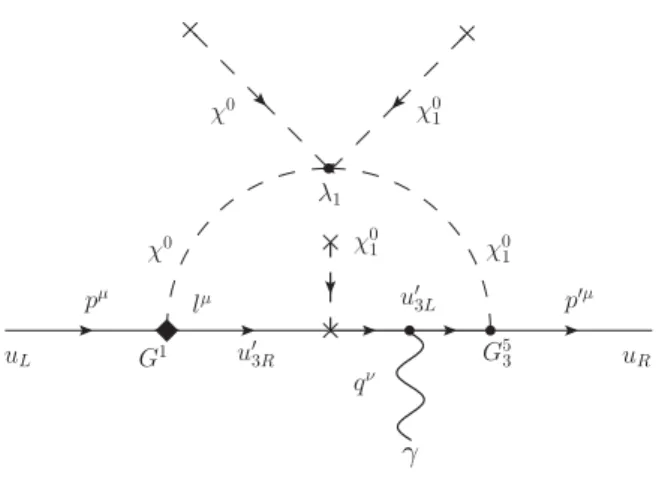
A.1 One loop diagram contributing to the electric dipole moment of the up-quark. The CP violating vertex is denoted with a diamond. . . 89 A.2 IntegralI(mu, mu′, m_χ, q2)whenq2 →0andm_u= 0.. . . 92 A.3 The quantityG5₃_|G1|sinφ×(1TeV/mχ)as function of the ratiomχ/mu′.

(9)

List of Tables

1.1 Assignment of PQ charges in the DFSZ model. . . 24

2.1 Assignment of quantum charges in the economical 3-3-1 model. . . 35 2.2 Assignment of quantum charges whenηis included. . . 41 2.3 The charge assignment forZ10andZ11that stabilize the axion, forα= 6. 44

(10)

Chapter 1 THE AXION: GENERALITIES

1.1 Introduction

Axions are fascinating hypothetical particles whose existence was proposed by S. Weinberg and F. Wilczek to give a resolution of the strong CP problem [1,2]. From its beginning, axion physics has motivated several experimental searches and the-oretical models. Since the invisible axions have extremely small coupling with the ordinary matter, their search has challenged the imagination and the experimental skills of the most of the physical community. Searches for solar, laser induced, relic and thermal axions have been performed. The majority of these experiments have been based on the Primakoff process which allows one photon to become an axion in the presence of an electromagnetic ﬁeld and vice versa. The absence of any axion signal has imposed strong limits on the axion properties, such as its mass and its coupling to two photons. Currently, there is a narrow window for the decay coupling constant of the axionfa,109GeV≤fa≤1012GeV, where the axion can be still found.

Although, from the effective theory point of view axion physics is relatively sim-ple, it involves a great amount of pieces of the physical knowledge, such as non-perturbative QCD effects (instantons) only to mention one, which require a more de-tailed study. Keeping it in mind, the motivation of this chapter is only to give a brief review of the main topics that axion physics involves and introduce some tools and ideas that will be necessary to get a better understanding of the rest of this thesis.

(11)

and 1.5 the classical Dine-Fischler-Srednicki-Zhitnisky (DFSZ) and Kim-Shifman-Vainshtein-Zakharov (KSVZ) axion models are reviewed. Furthermore, some tech-niques which will be used in the following chapters are introduced. Finally, in Sec.1.6 a concise review of some bounds on the axion properties coming from astrophysical and cosmological considerations is presented.

1.2 The

U

(1)

Problem and its Resolution

In the 1970s the strong interactions had a great puzzling problem, which be-came clear with the development of quantum chromodynamics (QCD). The QCD La-grangian entails an U(1) axial current, whose conservation is only broken by the quark mass terms. As consequence, the usual arguments of current algebra require a neutral pseudoscalar Nambu-Goldstone (NG) boson with a mass of the same order of magnitude as the pion mass as shown in Refs. [3,4]. But, this strongly interacting particle does not exist. This problem was called theU(1)problem by S. Weinberg.

To better understand this problem, consider the QCD theory with only three ﬂa-vors of quarks, u,d, ands. This is perfectly justiﬁed if we are interested in hadron physics at energies below_∼1GeV. Also to begin, let us assume that these quarks are massless. This is sensible because the massesmu,md,ms are small in the following

sense. The gauge couplinggof QCD becomes large at low energies. If we truncate the beta function after some number of terms, and integrate it, we find thatg becomes infinite at some finite, nonzero value of the MS (modified minimal-substraction renor-malization scheme) parameterμ[5,6]; this value is commonly calledΛQCD.

Measure-ments of the strength of the gauge coupling at high energies implyΛQCD ∼ 380±60

MeV [7]. Sincemu ≃ 0.0017,md ≃ 0.0039,ms ≃0.076in GeV [8] are much less than

ΛQCD this is a reasonable approximation to start with. With those approximations

done, and ignoring the effects of the quantum anomaly which will play a key role later, the Lagrangian of QCD is written as

LQCD =iχ†αiσμ(Dμ)_αβχβi+iξ_iα† σμDμαβξβi−

1 4G

aμν_Ga

μν, (1.1)

whereDμ =∂μ−igλaAaμ and Dμ =∂μ−igλaAaμ, with

λaαβ = −(λa)βα (a = 1,...,

8), are the covariant derivatives. The λaare the Gell-Mann matrices forSU(3)color group. We also have that χαi are left-handed Weyl ﬁelds in the 3 representation of

theSU(3)color group. Theα,β = 1,2,3and i= 1,2,3, are color and ﬂavor indices, respectively. Theξαi _{are left-handed Weyl ﬁelds in the}₃_{representation of the}_SU₍₃₎

color group, with color indices,α,β= 1,2,3and ﬂavor indicesi= 1,2,3. Notice that the spinor index carried by bothχ and ξ have been omitted. Finally, the color ﬁeld strengths,Ga

μν, are given by

(12)

whereAa

μrepresent the eight gluon ﬁelds, and thefabcare the structure functions of

theSU(3)group.

In addition to the SU(3) color gauge symmetry, this Lagrangian has a global U(3)_⊗U(3)ﬂavor symmetry

χαi → Lijχαj, (1.3)

ξαi _→ (R∗)i_jξαj, (1.4)

where L and R∗ are independent 3_×3 constant unitary matrices. In terms of the Dirac ﬁeld

Ψαi=

χαi

ξ†

αi

, (1.5)

Eqs. (1.3) and (1.4) read

PLΨαi → LijPLΨαj, (1.6)

PRΨ_αi → R_ijPRΨ_αj, (1.7)

where PL,R = 1₂(1∓γ5). Thus the global ﬂavor symmetry is often called U(3)L ⊗

U(3)_R. A symmetry that treats the left- and right-handed parts of a Dirac ﬁeld dif-ferently is said to be chiral.

Reconciliation of the experimental observations with theU(3)_L_⊗U(3)_R symme-try of the underlying Lagrangian is only possible if this symmesymme-try is spontaneously broken. Since in QCD there are no fundamental scalar ﬁelds that could acquire a nonzero VEV, the spontaneous symmetry breaking must happen through a quark-antiquark condensate. The simplest candidate is

0_|χαiaξ_bβj|0 =−1

6Λ 3_δ

αβδijǫab, (1.8)

wherea,b= 1,2are the undotted spinor indices; ǫab is the antisymmetric invariant

symbol of SU(2); and Λ is a parameter with dimensions of mass. The rest of the indices have the same meaning as in the Eq. (1.1). The condensate is unchanged only by transformations in the “vector” subgroup U(3)_V speciﬁed by R = L. Thus, U(3)_L_⊗U(3)_Ris spontaneously broken down toU(3)_V. To see that, note that under the transformations of Eqs. (1.3) and (1.4),

0_|χαiaξ_bβj|0 → Lik(R∗)jn0|χαkaξβn_b |0 ,

→ −1₆Λ3δαβǫab

LR†

i

j_. _(1.9)

(13)

side of Eq. (1.9) does not match that of Eq. (1.8), signifying that the axial generators are broken down.

At this point it is important to say that Eq. (1.8) is non-perturbative, i.e. 0_|χαia

ξ_jbβ _|0 vanishes at tree level and perturbative corrections also vanish, because of the chiral ﬂavor symmetry of the Lagrangian. Thus the value of Λ is not accessible in perturbation theory. It is expect thatΛ_∼ΛQCD, sinceΛQCD is the only mass scale in

the theory when the quarks are massless.

A low-energy effective Lagrangian [9], also known as chiral Lagrangian, for the nine expected NG bosons,18₋9, can be constructed in the following way. These NG bosons can be thought as long wavelength excitations of the condensate,

0_|χαiaξ_bβj|0 =−

1 6Λ

3_δ

αβδijǫabΣ (x)_ij, (1.10)

whereΣ (x)is an unitary matrix ﬁeld. Under aU(3)_L_⊗U(3)_Rtransformation,

Σ (x)_ij _→Lik(R∗)jnΣ (x)_kn. (1.11)

TheΣ (x)ﬁeld can be written as

Σ (x) = exp

−i 8

a=1

λa_πa_(x)

fπ −

iπ 9_(x)

f9

, (1.12)

where the Gell-Mann λ matrices are hermitian and normalized via Trλa_λb _{= 2δ}ab_;

theπa(x)(a= 1,...,8) are the hermitian NG ﬁelds; and thefπ andf9are parameters with dimensions of mass. fπ also is known as the pion decay constant, and it has the

measured values of92.4MeV [10].

The terms in the effective Lagrangian forΣ (x)can be organized by the number of derivatives that they contain. There is no allowed term with no derivatives because Σ†Σ = 1. As the Lagrangian must be U(3)_L_⊗U(3)_R invariant, there are no terms with only one derivative. There are two terms with two derivatives,

Lchiral ⊃ −

1 4f

2

πTr

∂μΣ†∂μΣ

−1₄F2∂μdet Σ†∂μ(det Σ). (1.13)

By requiring all nine NG ﬁelds to have canonical kinetic terms, theF parameter can be written in terms offπ and f9. To see this let us focus on theπ9dependence,

Σ (x) =

1₋ 1 f9

iπ9(x)

I₃_×₃₊_O_f−2

9

, (1.14)

det Σ (x) =

1₋ 1 f93iπ

9_(x)

+_Of₉−2, (1.15)

and

Lchiral=−

1 4

Tr[I₃_×₃_]_f_π2_{+ 9F}2_f−2

(14)

thus requiring the coefﬁcient of∂μ_π9_∂

μπ9 to be−1₂ yields

F2= 2 9

f₉2₋3

2f 2

π

. (1.17)

With all these done, the Lagrangian reads

Lchiral=−

1 4f

2

πTr∂μΣ†∂μΣ−

1 18

f₉2₋3

2f 2

π

∂μdet Σ†∂μ(det Σ) +.... (1.18)

In the real world, the three light quarks have small masses, thus the_LQCDgiven

in Eq. (1.1) contains

LQCD⊃ −Mijǫabχiαaξbjα +H.c., (1.19)

whereM is an arbitrary complex matrix.M can be made diagonal with positive real entriesmu,md, andmsvia anU(3)L⊗U(3)Rtransformation. In terms of the effective

Lagrangian,

Lchiral⊃Λ3Tr(MΣ +H.c.). (1.20)

Expanding in the NG ﬁelds, we obtain the following mass term

Lmass =−

1 4f2

π

Λ3TrMλa, λbπaπb, (1.21)

wherea,b= 1,...,9, andλ9 _≡(fπ/f9)13×3. It is usual to deﬁne

πa _≡ πaλa=√2 ⎛ ⎜ ⎜ ⎝ 1 √ 2π 3₊_√1

6π

8 _π+ _K+ π− ₋√1

2π 3₊_√1

6π

8 _K0

K− K0 ₋2₃π8

⎞ ⎟ ⎟ ⎠

+fπ f9

⎛ ⎜ ⎝

π9 ₀ ₀ 0 π9 0 0 0 π9

⎞ ⎟

⎠. (1.22)

To ﬁnd the eigenvalues of the mass-squared matrix in Eq. (1.21) let us write this explicitly

Lmass = −2Λ3fπ−2

(mu+md)π+π−+ (mu+ms)K+K−+ (md+ms)K0K0

mu

1

√

3π

8₊_π3₊_rπ9 2

+md

1

√

3π

8₋_π3₊_rπ9 2

+ms

₂

√

3π

8₊_rπ92

, (1.23)

wherer_≡fπ/f9. The squared masses of the charged NG bosons are easily read from Eq. (1.23)

m2_π± = 2Λ3f_π−2(m_u+m_d), (1.24)

m2_K± = 2Λ3f_π−2(m_u+m_s), (1.25)

m2

K0_K0 = 2Λ

3_f−2

(15)

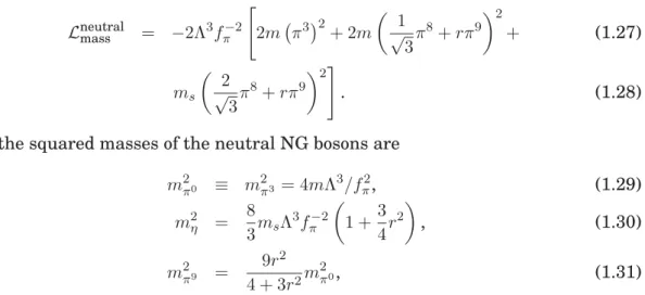
To simplify the calculation of the squared masses of the neutral NG bosons, setmu =

md=m≪ms. By doing so,

Lneutralmass = −2Λ3fπ−2

2mπ32+ 2m

1

√

3π

8₊_rπ92₊ _(1.27)

ms

2

√

3π

8₊_rπ92

. (1.28)

Thus the squared masses of the neutral NG bosons are

m2_π0 ≡ m2_π3 = 4mΛ3/f_π2, (1.29)

m2_η = 8 3msΛ

3_f−2

π

1 +3

4r

2_, _(1.30)

m2_π9 =

9r2 4 + 3r2m

2

π0, (1.31)

where, as it is usual, the neutral eigenstates asπ0,η,π9have been deﬁned. From the Eq. (1.31) we see that the maximum possible value ofm_π9 is

√

3m_π0, attained in the

limitf9 _→0. This particle does not appear in nature. This discrepancy between the-ory and experiment is known as theU(1)problem, as it has been mentioned before.

At ﬁrst glance, one might think that the Adler-Bell-Jackiw anomaly [11–14] pro-vides a possible solution to theU(1)problem, i.e. because the divergence of the axial currentJ₅μassociated with this symmetry gets quantum corrections from the triangle graph which connects it to two gluon ﬁelds, Aa, with quarks going around the loop Fig.1.2,

∂μ0|J5μ|Aa(p)Aa(q) =− g2_N 16π2

0GaμνGa_μνAa(p)Aa(q), (1.32)

whereN is the number of massless quarks andGa

μν = 12ǫμναβGaαβ, the axial current is not conserved. Thus there would not be anU(1)symmetry to worry about. In other

Aa

Ab p

q k1

k2

k3

J₅μ_∝γμγ5

γα

γβ

Figure 1.1:The lowest order Feynman graph leading to the chiral anomaly.

words, in the massless quark limit, although formally QCD is invariant underU(1) axial transformations,

(16)

the chiral anomaly affects the action,

δS =α

d4x ∂μJ5μ=−α g2_N 16π2

d4x ǫμναβTr[GμνGαβ], (1.34)

and thus theU(1)axial symmetry would not be a true quantum symmetry of QCD. However, since

− g

2_N 16π2ǫ

μναβ_Tr_[G

μνGαβ] = −

g2N 4π2ǫ

μναβ_∂ μTr

Aν∂αAβ−

2

3igAνAαAβ

≡ −g

2_N 4π2∂μW

μ_, _(1.35)

where

Wμ=ǫμναβTr

Aν∂αAβ−

2

3igAνAαAβ , (1.36)

the Eq. (1.32) can be reexpressed as

∂μ0|J5μ|Aa(p)Aa(q) = g2N

4π2∂μW

μ_. _(1.37)

Because of these identitiesδS is a pure surface integral

δS =₋αg 2_N 4π2

d4x ∂μWμ=−α

g2N 4π2

dσμWμ. (1.38)

Hence, one might think that!dσμWμ= 0, and thus, theU(1)axial symmetry would

appear as a symmetry of the QCD again. However, this it is not correct from the quantum point of view as showed by G. ’t Hooft [15,16].

To understand how it is possible that !dσμWμ = 0 and how this provides a

so-lution to theU(1)problem, consider the QCD vacuum structure. The classical QCD energy density is the sum of the square of the chromo-electric and chromo-magnetic fields. Thus the classical field configuration corresponding to the ground state is Ga_μν = 0. This happens whenever the vector potentialAμ, is a gauge transformation

of zero, i.e. Aμ ≡ Aaμλa = giU(x)∂μU†(x), whereU(x) is any SU(3)group

transfor-mation

U(x) = exp

iwa(x)λ

a

2 , (1.39)

witha= 1,...,8. Each conﬁguration correspond to a particular mapwa(x) of space-time into the eight-dimensional group manifold ofSU(3).

(17)

of generality because the following arguments will also apply to the SU(3) group, since this last contains theSU(2)group.

First, note that any2_×2special unitary matrixU can be written in the form

U =a4+i−→a .−→σ, (1.40)

wherea4 and the three vector−→a are real, and

− →_a2₊_a2

4= 1. (1.41)

Thus the aμ ≡ (−→a,a4) speciﬁes an Euclidean four-vector of unit length, aμaμ = 1,

and hence one point on three sphereS3. To determine the topology of the space-time, consider the possible vacuum conﬁgurations in the temporal gauge, A0 = 0. This restriction entails no loss of generality and means the unitary maps U(−→x) depend only on space. These maps, from one vacuum conﬁguration to the next, are local in space, and thus they must satisfy the boundary conditions

lim

|−→x_|→∞

U(−→x) =I, (1.42)

which do not depend on the direction at the spatial infinity. Hence, the maps are defined in a three dimensional space, with all of its directions at_∞identified. Thus the topology of the space-time is S3. Then, U(−→x) provides a map from the spatial three-sphere to the vacuum three-sphere, S3 _→ S3. These maps are characterized by a topological winding number n, which can be defined as the number of times that each sphere is mapped into the other. Given a smooth map U(−→x), its winding number can be written as [17]

n=₋ 1 24π2

d3x ǫijkTr[(U ∂iU) (U ∂jU) (U ∂kU)]. (1.43)

To verify that the equation above agrees with the previous deﬁnition of winding num-ber, consider the identity map (with winding number1)

U(_"xμ) =

x4+i−→x .−→σ ρ

=

cosχ+isinχcosψ isinχsinψe−iφ isinχsinψe+iφ _cos_χ₋_i_sin_χ_cos_ψ

, (1.44)

where

"

xμ= (sinχsinψcosφ,sinχsinψsinφ,sinχcosψ,cosχ), (1.45)

deﬁnes the polar anglesχandψ, and the azimuthal angleφ. Also,ρ_≡(xμxμ)1/2 has

been deﬁned. Plugging Eq. (1.44) in Eq. (1.43) is straightforward to get

(U ∂χU) (U ∂ψU) (U ∂φU) = −(U ∂ψU) (U ∂χU) (U ∂φU)

(18)

and

n=₋ 1 24π2

π

0 dχ

π

0 dψ

2π

0

dφ6sin2χsinψ Tr[I2×2] = 1, (1.47)

as it should be. Moreover, it is evident that ifφin Eq. (1.44) is replaced bynφ, that map will have a winding number equaln. With this done, it has been checked that the deﬁnition of the winding number given in Eq. (1.44) agrees with the previous deﬁnition of the winding number.

Now, consider the variation of n, δn, under smooth deformations of U(−→x). A deformationδU induces

ǫijkδTr[(U ∂iU) (U ∂jU) (U ∂kU)] = 3ǫijkTr[(U ∂iU) (U ∂jU)δ(U ∂kU)]

= ₋3ǫijkTr(U ∂iU) (U ∂jU)U ∂k

U†δUU†

= ₋3ǫijkTr(∂iU) (U ∂jU)U ∂k

U†δU, (1.48)

where the cyclic property of the trace,U†_U ₌I_and_δ_{(U ∂}_k_U_{) =}₋_{U ∂}_k_U†_δU_U†_have

been used. Continuing with the calculation

(1.48) = ₋3ǫijkTr∂k

(∂iU) (U ∂jU)U

U†δU₋∂k[(∂iU) (U ∂jU)U]

U†δU

= 3ǫijkTr(∂iU) (∂kU) (∂jU)δU+ (∂iU) (U ∂jU) (∂kU)

U†δU, (1.49)

where the surface term is zero after integrating because ofδU = 0at the boundary. Terms with two derivatives acting on a single U vanish when contracted with ǫijk_.

Now, usingU ∂jU† = −(∂jU)U† and (∂kU)U† = −U ∂kU†, followed by U†U = I, we

have that the remaining terms in Eq. (1.49) become

(1.49) = 3ǫijkTr[(∂iU) (∂kU) (∂jU)δU+ (∂iU) (∂jU) (∂kU)δU]. (1.50)

The two terms are now symmetric onj _↔ k, and thus cancel when contracted with ǫijk. Therefore, the winding numbernis invariant under smooth transformations of U(−→x).

The two previous results show thatSU(2)gauge theory has an infinity number of classical field configurations of zero energy, distinguished by an integern, and that these can not be smoothly deformed into each other. Furthermore, the existence of these non-equivalent classical field configuration of zero energy can be understood as the existence of different quantum vacuum states separated by energy barriers. To see why this is the case, suppose that U(−→x) and U"(−→x) have different winding numbers so that they can not be deformed into each other. The associated vector po-tentials,AμandA"μare both gauge transformations of zero, and so bothGμν andG"μν

vanish. However, if we try to smoothly deformAμintoA"μ, we must pass through

(19)

therefore do not vanish. These nonzero field strengths imply nonzero energy, which means that there is an energy barrier between the field configurationsAμandA"μ.

At this point, it would seem that we have many inequivalent theories, each start-ing from a different windstart-ing number, livstart-ing in a different Hilbert space with vacuum state_|Ωn , labeled by an integer. Thus, the key questions to make here are: Are there

many disconnected Hilbert spaces, one for each winding number?, and is the theory only invariant under gauge transformations that do not change the winding number? The answers depend on the existence of transition amplitudes between these differ-ent vacuum states. If no such transitions exist, unitary is realized in each Hilbert space, and we have many equivalent theories. On the other hand, if transitions be-tween Hilbert spaces do exist, all the (sub)Hilbert spaces must be included in order to have an unitary theory.

The answer to those questions is that actually, the winding number is not con-served by QCD; there is quantum tunneling between vacua of different winding num-ber, which are analyzed in the saddle-point approximation of the path integral [18], by expanding away of conﬁgurations of minimum action in Euclidean space. These conﬁgurations are called instantons. They mediate the tunneling. Their contribu-tions to the tunneling amplitude are of the order of

e−

8π2

g2 , (1.51)

wheregis the strong (QCD) coupling constant. Normally, such amplitude would lead to a negligible rate, but the QCD coupling constant can be very large in the infrared, effectively avoiding this typical exponential suppression of tunneling processes.

To better understand the appearance of those conﬁgurations let us show some of the main arguments that lead to those solutions without going into all details of the calculation.

The ﬁrst task will be to construct a Bogomolny bound on the Euclidean action

S = 1 2

d4xTr[GμνGμν], (1.52)

of a ﬁeld that obeys the boundary condition

lim

ρ→∞Aμ(x) =

i

gU(x"μ)∂μU†(x"μ), (1.53)

where x_"μ is deﬁned in Eq. (1.45), ρ = (xμxμ)1/2, and U("xμ) is a map with winding

numbern. Using the fact that Eq. (1.43) can be written as

n= 1 24π2

(20)

where∂μ=∂/∂xμandǫ1234 = +1. Now, using Eq. (1.53) in (1.54), the winding number

can be written in terms of the vector potential,

n= ig 3 24π2

dSμǫμναβTr[AνAαAβ]. (1.55)

Besides, using !dSμ ǫμναβTr[AνGαβ] = 0, the Gauss’s theorem, the Eq. (1.35), and

ǫμναβ_Tr_A

νGαβ+2₃igAνAαAβ = 2ǫμναβTrAν∂αAβ−2₃igAνAαAβ, the winding

num-ber becomes

(1.55) = g 2 16π2

dSμǫμναβTr

AνGαβ+

2

3igAνAαAβ

= g 2 8π2

d4x ∂μWμ

n = g

2 16π2

d4xTrGμνGμν

. (1.56)

The ﬁrst equality that has been used,!dSμǫμναβTr[AνGαβ] = 0, is due to that on the

surface at inﬁnity, the vector potential is a gauge transformation of zero, and so the ﬁeld strengthGαβ vanishes there. With this done, it easy to construct a Bogomolny

bound. First, note that

1 2Tr

Gμν±Gμν

2

=Tr[GμνGμν]±Tr

GμνGμν

, (1.57)

where GμνGμν = GμνGμν has been used. The left-handed side of Eq. (1.57) is

non-negative and so

d4xTr[GμνGμν]≥

d4xTrGμνGμν

. (1.58)

Therefore, ﬁnally, from Eq. (1.52), Eq. (1.56) and Eq. (1.58) the Bogomolny bound is given by

S _≥8π2_|n_|/g2. (1.59)

This bound gives us the minimum value of the Euclidean action for a solution of the Euclidean field equations that mediates between a vacuum configuration with winding numbern₋ atx4 =−∞ and a vacuum configuration with winding number n+=n₋+natx4 = +_∞.

The instanton solution can be found by resolving

Gμν = (signn)Gμν, (1.60)

for a map with winding numbern= 1. To ﬁnd it explicitly let us make the following ansatz [19]

Aμ(x) =

i

gf(ρ)U(x"μ)∂μU

†₍_"_x

(21)

wheref(_∞) = 1, so that the solution obeys the boundary conditions;f(0) = 0, since Aμ should be well deﬁned at ρ = 0; and U(x"μ) is given by Eq. (1.44). Plugging

Eq. (1.61) in Eq. (1.60), it is straightforward to ﬁnd

f(ρ) = ρ 2

ρ2₊_a2, (1.62)

wherea, the size of the instanton, is a constant of integration. The instanton solution is also parameterized by the location of its center; here it has been used the space-time origin, but the translation invariance allows us to displace it.

Now, since the vacua of different winding numbers can be reached via instantons, as showed above, we come to two important conclusions. Writing these in a short way,

• The chiralU(1)symmetry is no more a symmetry of the QCD Lagrangian and thus theU(1)problem does not exist anymore.

• The QCD Lagrangian has a new parameter,θ.

The ﬁrst conclusion is easily reached. The existence of instantons affect the chargeQ5 =!d4x ∂μJ5μ in the sense that the charge after the instanton differs from the charge before the instanton. This can be seen in the following way

∆Q5 =

d4x ∂μJ5μ

= g 2_N 8π2

d4xTrGμνGμν

= _±2N, (1.63)

where the Eqs. (1.34) and (1.56) have been used. Note that, although the instanton solution has been computed using analytic continuation to Euclidean space-time, the tunneling process between different vacua take place in the Minkowski space-time. Furthermore, being topological equations, Eqs. (1.32), (1.56) and (1.59) hold both in Euclidean and Minkowski space-times, since they are independent of the metric.

In conclusion, in the limit of N massless quarks, although the QCD Lagrangian has the global symmetry

U(N)_L_⊗U(N)_R _∼ SU(N)_L_⊗SU(N)_R_⊗U(1)_L_⊗U(1)_R

∼ SU(N)_L_⊗SU(N)_R_⊗U(1)_V_⊗U(1)_A, (1.64)

the instanton contribution violates theU(1)_Asymmetry, and thus it provides a solu-tion to theU(1)problem.

(22)

instantons, the physical vacuum state must be a linear superposition of all states of zero energy and different winding numbers, _|Ωn . Its precise form is determined

by gauge invariance. Under a gauge transformation _U which changes the winding number by one unit, we have

U |Ωn =|Ωn+1 . (1.65)

None of these states are physical since they can be transformed into one another by a gauge transformation. The vacuum state is the one on which a gauge transformation can at most result in a phase transformation. This ﬁxes the physical vacuum to be given by the Bloch superposition

|Ωθ = n

e−inθ_|Ωn , (1.66)

which is designed such that

U |Ωθ =eiθ|Ωθ . (1.67)

Therefore, the true vacuum state of the SU(3) gauge theory depends on an angle θ, deﬁned module 2π. This new parameter has for effect to alter the Lagrangian by a surface term which does not appear in the equations of motion, yielding the effective Lagrangian in Minkowski space

LSU(3)=Tr

−1₂GμνGμν− g

2_θ 16π2G

μν_G

μν . (1.68)

The appearance of the extra term in the Lagrangian is better understood by consider-ing the Euclidean path integral formalism. To do that, suppose that we are interested in starting with a particular theta vacuum|Ωθ , and ending with a (possibly different)

theta vacuum_|Ωθ′ . Then from Eq. (1.66)

Ωθ′|Ω_θ =Z_θ′

←θ(J) = n−,n+

ei(n+θ′−n−θ)_Z

n+←n−(J), (1.69)

where

# Ωn+

Ωn−$=Zn+←n−(J) =

DAn+−n− e−

S+JA_, _(1.70)

withJA _≡!d4_x_Tr[Jμ_A

μ], and the subscript on the ﬁeld differential means that we

integrate only over ﬁelds with that winding number. Now, deﬁningn+=n₋+n, and summing overn₋we have

Zθ′

←θ(J) =δθ′−θ n

einθ

DAne−S+JA. (1.71)

The δ(θ′₋θ) in the above equation means that the value of θ is time independent. Thus we can drop the delta function, and just deﬁne

Zθ(J)≡ n

einθ

(23)

Next, combining the sum overnand the integral overAninto an integral over allA,

and using Eq. (1.56) results

Zθ(J) =

DA exp

d4xTr

−1₂GμνGμν+

ig2θ 16π2G

μν_G

μν+JμAμ , (1.73)

thus theθangle appears as the coefﬁcient of an extra term in theSU(3)Yang-Mills Lagrangian. When we return to the Minkowski space (by settingx0 =it), we obtain the Lagrangian given in Eq. (1.68)

1.3 The Strong CP Problem and its Resolutions

As showed in the previous section, the QCD Lagrangian has a new parameter θ. This parameter can have any value between 0 and 2π, and it is hoped to be of order one,_O(1). However, the absence of a measurable electric dipole moment for the neutron,_|dn|<2.9×10−26ecm [20], suggests that

θ0.7_×10−11, (1.74)

whereθ_≡θ₋arg det Mq, being Mq the quark mass matrix. The reason why this

pa-rameter is so small is known as the strong CP problem. Notice that in the Eq. (1.74), the parameter used wasθinstead ofθ. This is so, because the physical parameter is θas it will be explained later.

Although there is no experimental evidence that the strong interactions violate either P and CP symmetries, the QCD is capable of breaking these symmetries both spontaneously and explicitly. The former through the quark condensate given in Eq. (1.8), the latter through interactions which violate these symmetries. Here, we concentrate in the last case.

Explicitly breaking comes from the term

− g

2_θ 16π2Tr

GμνGμν

. (1.75)

This term is clearly odd under P and CP. Note that

ǫμναβGμνGαβ ∼ǫijkG0iGjk, (1.76)

and making an analogy with the electromagnetic ﬁeld, whereǫμναβFμνFαβ ∼ǫijkF0iFjk

=−→E .−→B, the transformation of Eq. (1.75) under P and CP is evident. Here, it is also important to note that the parameter in Eq. (1.75) is not a physical parameter. This can be understood if we consider the quark mass term in the QCD Lagrangian. Sup-pose that we have only a quark ﬁeld given by Eq. (1.5) with the mass term

Lmass = −mχξ−m∗ξ†χ (1.77)

(24)

where m = _|m_|eiφ_{. Then, a}_U₍₁₎

A transformations given by Eq. (1.33) changesφ to

φ₋α/2. Sinceθ simultaneously changes to θ₋α/2, we see that θ₋φ is invariant. Thus the actual physical parameter isθ₋φ. With more quarks ﬁelds, the mass term is_Lmass =−(Mq)_ijχiξj+H.c., and the physical parameter is

θ = θ₋arg detMq

≡ θQCD−θQFD, (1.79)

where the deﬁnitionsθQCD ≡θand θQFD ≡arg detMq have been done. The acronym

QFD inθQFDmean Quantum Flavor Dynamics.

Having showed that the θin the Lagrangian violates the P and CP symmetries, consider the places where strong CP violation can manifest itself. Two places where it is possible, in principle, to see CP violation are the P- and T-violating η _→ 2π decay [21] and the electric dipole moment dn [20]. As it is well known, the most

stringent limit onθis set by the neutron electric dipole moment (NEDM).

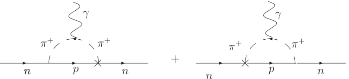
To give one estimate for NEDM, we follow Ref. [22]. The diagrams that most contribute to the NEDM are shown in Fig. 1.3. These diagrams are enhanced by a lnΛ2_/m2

π

∼ 4.2, where Λ _∼ 4πfπ is the ultraviolet cutoff in the effective theory.

No other contributing diagrams have this enhancement. Of course, this number is not impressively large number, and thus we can not be certain that the remaining contributions are not signiﬁcant. However, here we restrict ourselves to consider only these kind of diagrams as it was done in Ref. [22]. To calculate these contributions it

n

π

+

π

+

γ

p

+

n

_n

γ

n

p

π

+

π

+

Figure 1.2: Diagrams contributing to the electric dipole moment of the neutron. The CP violating vertex is denoted with a cross.

is needed to know the couplings ofnpπ+_{. The Lagrangian for this interaction is given} by

LπN N = −i

√

2 (gAmN/fπ)π+pγ5n+π−nγ5p, (1.80)

LθπN N = −

√

(25)

wheremN is the neutron mass,≈939.56MeV,fπ = 92.4MeV,gA≃1.27,

c+ =

m_Ξ0−m_Σ0

ms−1₂mu−1₂md ≃

1.7, (1.82)

m = mumd mu+md ≃

1.2MeV. (1.83)

Without going into the details, the amplitude for the diagrams in the Fig.1.3

T =₋4eθgAc+m/f π2

ε∗_μuSμνqνiγ5u Λ

0 d4l (2π)4

1 (l2₊_m2

π)2

, (1.84)

whereq is the momentum of the photon, andSμν ₌ i

4[γμ, γν]. Using standard tech-niques

dn=

eθgAc+m 8π2_f2

π

lnΛ2/m2_π_≃3.2_×10−16θ ecm. (1.85)

The experimental upper limit is_|dn| < 2.9×10−26 ecm [20], thusθ < 0.9×10−10.

Note that there are a lot of other estimates of the NEDM using different methods [23– 25], but the important thing here is that in all of these methods the parameterθ is extremely small.

Before going to the different solutions to the strong CP problem, let us rephrase it in different ways. First, it is a CP hierarchy problem. Weak CP violation inK0₋K0 systems is characterized byεparameter which is of order of10−3, whereas strong CP is measured by the very small parameter θ. Also, it is a problem of ﬁne-tuning in the sense that the combinations of two non physical parametersθQCD andθQFDis so

small irrespective of the arbitrary value ofθQCD.

If QCD is supposed to be the correct theory of the strong interactions, a solution to the strong CP problem must be found. Several “solutions” have been proposed. These can be classiﬁed as follows

• Unconventional dynamics.

• Spontaneously broken CP.

• An additional chiral symmetry.

Solutions based on unconventional dynamics suggest that the boundary condi-tions that give rise to theθvacuum are an artifact [26], however this does not provide one solution to theU(1)problem. Other approaches use the periodicity of the vacuum energy to deduce thatθ vanishes [27]. This type of approach is not satisfactory be-cause it fails to motive the minimization of the vacuum energy.

(26)

the weak CP symmetry violation in the neutral K mesons system and B _→ K+_π−

decay [8], and hence the potential is arranged to break CP spontaneously. In these models must be guaranteed that the parameterθ is small enough to be within the experimental value after radiative corrections are done. In other words [28],

θ_∼ 1 16π2∆f

2 _{(loop integrals)}_≤_0.7_×₁₀−11_, _(1.86)

where∆f2 _{is the product of coupling constants and the Feynmann loop integrals are} of _O(1). Therefore, ∆f2 must be small enough to satisfy the experimental bound. Along this line, many ideas were proposed [29–31]. These ideas have difﬁculties in satisfying the bounds of the current CP violation data, for example, ﬂavor changing neutral currents (FCNC) and domain walls [32]. Another drawback for this type of approach is that the experimental data are in excellent agreement with the Cabibbo-Kobayashi-Maskawa model (CKM model), a model where CP is explicitly broken.

However, there is a type of weak CP violation [33, 34], known as Nelson-Barr, that mimics CKM type CP violation even though the fundamental reason for the CP violation is spontaneous. To understand how this mechanism works we follow here S. M. Barr [34]. Suppose that in a model the fermions can be classiﬁed in two sets:F consisting of fermions with the sameSU(3)_⊗SU(2)_⊗U(1)quantum numbers as the ordinary light families, and R consisting of a real set of representations of SU(3)_⊗SU(2)_⊗U(1)(Rmay content complex representations as long as it contains an equal number of conjugate representations.) Then θ will be zero at tree level if two conditions are satisﬁed

• TheSU(2)_⊗U(1)breaking vacuum expectation values (VEVs) appear only in F₋F Yukawa terms not inF₋R orR₋Rterms.

• CP- nonconserving VEVs appear only inF ₋RYukawa terms, not inF ₋F or R₋Rterms.

To illustrate the idea, consider augment the standard model chiral quarks with vector-like weak doublet with standard model hypercharge, and two vector-like weak singlets of charges2/3and₋1/3:

R=

R1 R2

1/3

, R=

R1 R2

−1/3

, R′₁₄_/₃+(R′₁)₋4/3,

R′₂₋₂_/₃+(R′₂)2/3. (1.87)

(27)

mass matrix

d, R2, R′2

⎛ ⎜ ⎝

Hd S 0

0 M 0

S′ 0 M′

⎞ ⎟ ⎠

⎛ ⎜ ⎝

d R2 R′₂

⎞ ⎟

⎠, (1.88)

where Hd , M, M′ are real, and S , S′ are complex. The determinant of mass

matrix,Hd (M M′), is real. A similar matrix obtains in the2/3charged sector. There

will be loop corrections to the phase of the determinant which will induce a non-zero value of θ. These will be model dependent. In the particular model of the Ref. [33] they are shown to be small.

Introducing an additional chiral symmetry is a very natural solution for the strong CP problem, as this is chiral, it rotates thisθparameter away. There are two ways to introduce this symmetry:

• The up-quark is massless [35].

• The standard model has an additional globalU(1)chiral symmetry, known as U(1)_PQ [36,37].

The ﬁrst possibility works in the following way. The path integral for QCD with one quarkΨ(up-quark) massless is

Zθ(J) =

DA_DΨ_DΨ

×exp i

d4xTr

iΨγμDμΨ−

1 2G

μν_G μν−

g2_θ 16π2G

μν_G

μν+JμAμ .

(1.89)

Under aU(1)Atransformation

Ψ _→ e−iαγ5_Ψ, _(1.90)

Ψ _→ Ψe−iαγ5

, (1.91)

the integration measure picks up a phase factor

DΨ_DΨ_→exp

−i

d4x g 2_α 16π2G

aμν_Ga

μν DΨDΨ, (1.92)

because theU(1)Asymmetry is anomalous as showed in the previous section. Thus

Zθ(J) →

DA_DΨ_DΨ

×exp i

d4xTr

iΨγμDμΨ−

1 2G

μν_G

μν−θ+ 2α

g2 16π2G

μν_G

μν+JμAμ .

(28)

Hence, θ can be taken away from the QCD Lagrangian by doing a chiral transfor-mation with α = ₋θ/2. The question for this possibility is, “is the massless up-quark phenomenologically viable?” It is widely believed that within the context of the lowest-order chiral perturbation theory,mu= 0is inconsistent with the observed

mesons and baryon masses, ρ₋ω mixing, Σ0₋Λ mixing,η _→ 3π, and lattice QCD calculations [38–42]. Those calculations show that the ratio betweenmu andmdis

mu/md= 0.410±0.036. (1.94)

Therefore this possibility is disfavored.

The second possibility, which seems to be the most attractive one, is when the additional global U(1)_PQ chiral symmetry introduced into the entire Lagrangian is spontaneously broken down. Thus a new pseudo-NG boson called the axion, a(x), appears in the physical scalar spectrum. Because the axion is the NG boson of the U(1)_PQ symmetry, it shifts

a(x)_→a(x) +αfa, (1.95)

when anU(1)_PQ transformation is done. Thefa parameter in the Eq. (1.95) is

asso-ciated with the breaking of theU(1)_PQsymmetry. In other words, this solution try to mimic dynamically the shift symmetryθ_→θ+ 2α of the previous “solution”.

Under the symmetry transformation given in the Eq. (1.95), the effective La-grangian undergoes the transformation

δ_Leff=−

αA

32π2ǫμνρσG

aμν_Gaρσ_, _(1.96)

whereAis a dimensionless constant of order unity, characterizing the anomaly. Then the terms in the effective Lagrangian involvinga(x)are

La=−

1 2∂μa∂

μ_a

−_32π1₂Aa_f

a

ǫμνρσGaμνGaρσ+. . . . (1.97)

Comparing Eqs. (1.89) and (1.97) for a a(x) constant, it can be seen that all observ-ables will be functions not ofa(x)andθseparately, but only ofθ+Aa/fa. If everything

in the theory apart from the theta term (1.89) and (1.97) conserves P and CP, then effective potential will be even in θ+Aa/fa, and it will have a stationary point at

θ+Aa/fa= 0, preserving the conservations of P and CP. This is basically the

philos-ophy behind the the PQ mechanism.

(29)

1.4 DFSZ Axion

Since this model is identical to that of Peccei and Quinn (PQ) [37] model except for the addition of a complex scalar ﬁeld,Φ, which is a singlet under theSU(2)_L_⊗U(1)_Y gauge group (theSU(2)_L_⊗U(1)_Y group is known as the standard model (SM) model group), we consider ﬁrstly that model.

The fermionic matter content of the PQ model is the same as in the SM model, i.e. neither leptons nor quarks are added. The way as theU(1)_PQ symmetry is im-plemented is introducing a new Higgs ﬁeld, Hu, which couples only to the quarks.

To avoid naturally tree-level ﬂavor changing neutral current effects (FCNC), each Higgs doublet is coupled to one quark charge sector. With this, the relevant Yukawa interactions read

LY =GuijQLiuRjHu+GdiiQLidRiHd+GeiiLLieRiHd+H.c., (1.98)

where

QLi= (ui,di)T , LLi= (νi,ei)T, Hd=H_d+,Hd0

, Hu =Hu0,Hu−

, (1.99)

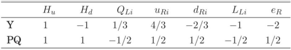
and i, j = 1, 2, 3. The Yukawa Lagrangian given in Eq. (1.98) has the required global PQ symmetry. The charge assignment is given in the Table (1.1). With two

Table 1.1: Assignment of PQ charges in the DFSZ model. Hu Hd QLi uRi dRi LLi eR

Y 1 ₋1 1/3 4/3 ₋2/3 ₋1 ₋2 PQ 1 1 ₋1/2 1/2 1/2 ₋1/2 1/2

Higgs scalar ﬁelds, the most general scalar potential which is invariant under the PQ symmetry is given by

VHu,d =

−μ2_aH_a†Ha+λaa

H_a†Ha

2

+λudHu†HuH_d†Hd

+λ′_udH_u†HdH_d†Hu . (1.100)

When bothHd and Hu acquire vacuum expectation values (VEVs), the PQ

symme-try is broken at the same scale as the electroweak symmesymme-try. SinceVPQ breaks the

SM group it can not be larger thanG−_F1/2, whereGF is the Fermi coupling constant.

Thus the axion has mass and coupling strength that make it ruled out by the experi-ments [47].

As it was previously said, to overcome this difﬁculty in this model one singlet scalar Φis introduced. BecauseΦis a singlet under the SM group, it can acquire a VEV,VΦ, which is required to be larger than G−F1/2, i.e. VΦ ≫ G−

1/2

(30)

couplings of the axion to the matter (∝ 1/VΦ) become suppressed and in agreement with experiments. It is the reason why this type of axion is known as the “invisible” axion.

The singlet Φﬁeld can gain PQ charge coupling to the ﬁelds Hu and Hd in two

different ways. The former is a cubic interaction

μH_uiǫijHdjΦ +H.c., (1.101)

whereμis a constant with mass units andǫij is the completely antisymmetric symbol

ofSU(2). This type of interaction was considered in the Ref. [44]. And the second possibility, which is considered here, has a quartic term

λP QHuiǫijH_djΦ2+H.c., (1.102)

where λP Q is a dimensionless constant. This was considered in the Ref. [43]. The

cubic interaction can be set to zero naturally, by imposing the discrete symmetry Φ_{→ −}Φ. In the case with a quartic term the scalar potential is simply

Vclassic=VHu,d+VΦ+λPQH

i

uǫijH_djΦ2+H.c., (1.103)

whereVΦ

VΦ =−μ2ΦΦ†Φ +λΦ

Φ†Φ2. (1.104)

Now, it is the time to give an explicitly expression to the axion. To do that, let us before discussing brieﬂy the procedure that has been used throughout this work. At the classical level, the squared masses of the scalars in the theory are the eigenvalues of the following matrix [5]

m2_ij = ∂ 2_V

classic

∂φi∂φj

φi=Vi

, (1.105)

where theφi in Eq. (1.105) makes reference to the components of the scalar ﬁelds of

the model, for instance ReH0

u, ImHu0, Re Hu−, Im Hu−, etc. The Vis are the VEVs of

the scalar ﬁelds. It is important to say that

∂Vclassic

∂φi

φi=Vi

= 0, (1.106)

because φi = Vi minimizes Vclassic. After ﬁnding the eigenvalues and eigenstates of

the matrix in Eq. (1.105), it is necessary isolate the physical axion ﬁeld, which at the classical level is massless, from the would be NG bosons which in the unitary gauge will become the longitudinal components of the massive gauge bosons. In general, the would be NG bosons are generated by some linear combination of the rows of the matrix

(31)

whereiruns on the total number of real ﬁelds in the model,aruns on all generators of the gauge groups, gas are the coupling constants of the gauge groups, and theTa

matrices are given by [9]

Ta=

−Imτa ₋Reτa Reτa ₋_Im_τa

. (1.108)

The τa_{s are the generators of the gauge group. To put all that in a short way, the}

axion ﬁeld,a, must satisfy

i

ai∗Fbi = 0, ∀b, (1.109)

whereai are the components of the axion ﬁeld. These are given by

a=

n

cn∗bn, (1.110)

wherebnare the eigenstates that are a base to the linear vector space of the massless

scalars. Thecnare constants which are found using the Eqs. (1.109).

Now, applying the above procedure to the DFSZ axion, we have

Hu =

⎛ ⎜ ⎜ ⎜ ⎜ ⎝

ReH_u0 ReH−

u

ImH_u0 ImH_u−

⎞ ⎟ ⎟ ⎟ ⎟

⎠, Hd= ⎛ ⎜ ⎜ ⎜ ⎜ ⎝

ReH_d− ReH0

d

ImH_d− ImH_d0

⎞ ⎟ ⎟ ⎟ ⎟ ⎠, Φ =

ReΦ ImΦ

. (1.111)

Thus we have ten real scalar ﬁelds. The generators of the gauge groups,SU(2)_L_⊗ U(1)_Y, in the real representations are

T1 = −1 2 ⎛ ⎜ ⎜ ⎜ ⎜ ⎝

0 0 0 1 0 0 1 0 0 ₋1 0 0

−1 0 0 0

⎞ ⎟ ⎟ ⎟ ⎟ ⎠, T

2 ₌ −1 2 ⎛ ⎜ ⎜ ⎜ ⎜ ⎝

0 ₋1 0 0 1 0 0 0 0 0 0 ₋1 0 0 1 0

⎞ ⎟ ⎟ ⎟ ⎟ ⎠,

T3 = −1 2 ⎛ ⎜ ⎜ ⎜ ⎜ ⎝

0 0 1 0 0 0 0 ₋1

−1 0 0 0 0 1 0 0

⎞ ⎟ ⎟ ⎟ ⎟ ⎠, T

4 ₌₋_Y

s ⎛ ⎜ ⎜ ⎜ ⎜ ⎝

0 0 ₋1 0 0 0 0 ₋1 1 0 0 0 0 1 0 0

⎞ ⎟ ⎟ ⎟ ⎟

⎠. (1.112)

where the Ys are the hypercharges of the scalar ﬁelds given in the Table 1.1. The

vector of the VEVs is

V = (Vu,0,0,0,0,Vd,0,0,VΦ,0)T . (1.113)

Finally, using the Eqs. (1.105-1.107), (1.109-1.110), and (1.112) the axion reads [43]

a(x) = 2VuVdVuImHd0+VdImHu0

−V_EW2 VΦImΦ

×VEWVEW2 VΦ2+ 4Vu2Vd2

(32)

whereVEW ≡

V2

u +Vd2

1/2

. Note that in the limitVφ≫Vu,Vd,

a(x)_{≃ −}ImΦ +2VuVd/VΦVEW2 VuImHd0+VdImHu0

, (1.114)

i.e. the axion is primarily composed of theΦﬁeld.

Although, the axion is massless at tree-level, it gains mass because the U(1)_PQ symmetry is anomalous. QCD effects (such as instantons [15]) that violate U(1)_PQ give a small mass to the axion [48] given by

m2_a=f_π2/f_a2m2_πN2Z(1 +Z)−2, (1.115)

where Z = mu/md ≃ 0.56 (mu and md are the u- and d-quark masses respectively),

N is the number of quark doublets, mπ and fπ ≈ 130MeV are the mass and decay

constant of theπ0_. _f

ais the axion decay constant given in this model by [43]

fa= (2VEW)−1

V_EW2 V_Φ2+ 4V_u2V_d21/2. (1.116)

Astrophysical and cosmological considerations limitfato be between

109 GeV_≤fa≤1012GeV. (1.117)

1.5 KSVZ Axion

This type of model for the axion is simpler than the DFSZ axion model and was introduced by the ﬁrst time in the Refs. [45, 46]. The gauge group is the same as the SM group and except for weak singlets both Q quark and σ scalar, the matter content is the same as in the SM one. To introduce naturally the PQ symmetry aZ2 symmetry is imposed, such that

Z2 : QL→ −QL, QR→QR, σ → −σ; (1.118)

and all the other ﬁelds are invariant. Notice that this symmetry guarantees the absence of the bare-mass termmQQ. The invariant Yukawa term ofQand the Higgs potentialV are simply

LYQ = Y QLQRσ+H.c., (1.119)

V = ₋μ2_HH_d†Hd−μ2σσ†σ+λH

H_d†Hd

2

+λσ

σ†σ2+λHσ

H_d†Hd σ†σ

, (1.120)

whereHdis the SM Higgs and it is given by the Eq. (1.99).

In this model the PQ symmetry is given by

Q_→eiγ5α_Q, _σ

(33)

which is used to rotate away the term

Lθ =

g2θ 16π2Tr

GμνGμν

. (1.122)

It is important to say that this is possible provided theQquark belongs to a nontrivial representation ofSU(3)_C.

The ﬁeldσdevelops a non-vanishing vacuum expectation value,

|σ_{| ≡}Vσ=μσ/

%

2λσ, (1.123)

thus the model has a new scalarσR with mass μσ√2 and a pseudoscalar, the axion,

whose mass vanishes in the classical approximation. The new quarkQgain a mass equal toY Vσ. In order to the axion phenomenology agree with the cosmological and

astrophysical data Vσ ≫ VHd. More precisely Vσ 10

9 _{GeV. Thus the} _Q _{quark is} not directly observable in low energy experiments. The only interesting effect in low energy is determined by the heavy quark loop which induces a term in the effective Lagrangian

g2 16π2

a(x) Vσ

TrGμνGμν

, (1.124)

wherea(x)is the axion ﬁeld and it is related to the original ﬁeldσ(x)in the following way

σ(x) = 2−1/2(Vσ+σR)eia(x)/Vσ. (1.125)

The interaction axion-gluon in the Eq. (1.124) results in the substitution of the pa-rameterθbyθeff=θ+a(x)/Vσ and the vacuum expectation value ofa(x)can be seen

to cancel the originalθ.

In this model, the term in the Eq. (1.124) also gives mass to the axion [46]

m2_a= f 2

πm2π

√

2V2

σ

mumd

m2

u+m2d

, (1.126)

similarly to the DFSZ model.

1.6 Searches for the Axion

During the last thirty years, several experiments searching for signals of the ax-ion existence have been performed. Among the most important ones are Cern Axax-ion Solar Telescope (CAST), Tokyo Axion helioscope experiment, Brookhaven-Fermilab-Rutherford-Trieste (BFRT) collaboration, SOLAX, COSME, DAMA. The majority of the previous experiments are based on the (reversed) Primakoff effects, i.e. a + γvirtual→γ, where the axion interacts with a virtual photon provided by a transversal

(34)

As seen from the Earth, the most important and strongest astrophysical source for axion is the core of the Sun. Particles like the axion have the following coupling to two photons

Laγγ =

gaγγ

4 FμνF

μν_a₌

−gaγγE.Ba, (1.127)

whereFμν is the electromagnetic ﬁeld-strength tensor,Fμν its dual, and E and B the

electric and magnetic ﬁelds, respectively. The coupling constantgaγγis given by

gaγγ =

α 2πfa

E N −

2 3

4 +z 1 +z

= α

2π

E N −

2 3

4 +z 1 +z

1 +z

z1/2 ma

mπfπ

, (1.128)

wherez=mu/md≃0.56,αis the ﬁne-structure constant;E andN, respectively, are

the electromagnetic and color anomaly of the axial current associated with the axion ﬁeld. EandN are given by [49]

N = XiT(Ri), E = XiQ2iD(Ri), (1.129)

whereT(Ri)is the Dynkin index of theSU(3)C representation of the quarkqi,D(Ri)

is the dimension of the representation, Qi and Xi, respectively, are the electric and

PQ charges of the quarkqi. In general,gaγγis model-dependent.

The coupling in Eq. (1.127) allows the production of axions from thermal photons in the fluctuating electromagnetic fields of the stellar plasma. Thus if axions scape from the Sun core, these reach the Earth, and in principle, they can be detected using the reversed Primakoff effect, since the axion interacts with electromagnetic field producing X-rays. This type of experiment is known as the axion helioscope experiment and the idea was firstly proposed by P. Sikivie in 1983 [50]. The absence of the axion signals resulted in upper limits ongaγγ[51]

gaγγ ≤ 6×10−10GeV−1 forma<0.03eV, (1.130)

gaγγ ≤ 6.8−10.9×10−10GeV−1forma<0.3eV, (1.131)

for the Tokyo Axion helioscope experiment, and

gaγγ ≤0.88×10−10GeV−1forma<0.02eV, (1.132)

at the 95% conﬁdence level for the CAST [52]. Using different experimental tech-niques the collaborations SOLAX, COSME and DAMA achieved similar limits [53– 56]

gaγγ ≤ 2.7×10−9 GeV−1 (SOLAX), (1.133)

gaγγ ≤ 2.8×10−9 GeV−1 (COSME), (1.134)

gaγγ ≤ 1.7×10−9 GeV−1 (DAMA), (1.135)

(35)

Other important and strong type of limits come from Globular-Cluster stars and the supernova (SN) 1987A. Roughly speaking, these limits are based on energy-loss argument which say, in a short way, that the existence of new particles like the axion coupling to the photons, leptons and hadrons would be a new channel for energy loss in the stars, and thus, the evolutions of these objects should signiﬁcantly change. Studies considering these factors have been performed obtain strong limits ongaγγ,

gaγγ <10−10GeV−1, (1.137)

comes from the Globular-Cluster [57] stars and

fa<4×108GeV andma16meV, (1.138)

comes from the SN 1987A [58].

Finally, from cosmology it was found that a general lower limit could be placed on the axion mass. At the time of the big bang, axions would be produced in a signiﬁcant amount by different mechanisms as misalignment, or the decay of axionic strings. Al-though there are still substantial uncertainties on the calculations of the relic axion abundance, an estimate for the total contributions to the energy density of the uni-verse from axions created via the vacuum misalignment method can be expressed as [59,60]

Ωa∼

5μeV

ma

7/6

, (1.139)

which put a lower limit on the axion mass ofma≥10−6 eV because any lighter axion

(36)

Chapter 2 NATURAL PECCEI-QUINN

SYMMETRY IN THE 3-3-1 MODEL

WITH A MINIMAL SCALAR SECTOR

2.1 Introduction

The standard model (SM) of the elementary particles physics successfully de-scribes almost all of the phenomenology of the strong, electromagnetic, and weak interactions. However, from the experimental point of view, the need to go to physics beyond the standard model comes from the neutrino masses and mixing, which are required to explain the solar and atmospheric neutrino data. On the other hand, from the theoretical point of view, the SM cannot be taken as the fundamental the-ory since some important contemporary questions, like the number of generations of quarks and leptons, do not have an answer in its context. Unfortunately we do not know what the physics beyond the SM should be. A likely scenario is that at the TeV scale physics will be described by models which, at least, give some insight into the unanswered questions of the SM.

A way of introducing new physics is to enlarge the symmetry gauge group. For example, the gauge symmetry may beSU(3)C⊗SU(3)L⊗U(1)X, instead of that of the