A stochastic discount factor approach to asset pricing using panel data asymptotics

❊♥s❛✐♦s ❊❝♦♥ô♠✐❝♦s

❊s❝♦❧❛ ❞❡

Pós✲●r❛❞✉❛çã♦

❡♠ ❊❝♦♥♦♠✐❛

❞❛ ❋✉♥❞❛çã♦

●❡t✉❧✐♦ ❱❛r❣❛s

◆◦ ✼✶✼ ■❙❙◆ ✵✶✵✹✲✽✾✶✵

❆ ❙t♦❝❤❛st✐❝ ❞✐s❝♦✉♥t ❢❛❝t♦r ❛♣♣r♦❛❝❤ t♦ ❛s✲

s❡t ♣r✐❝✐♥❣ ✉s✐♥❣ ♣❛♥❡❧ ❞❛t❛ ❛s②♠♣t♦t✐❝s

❋❛❜✐♦ ❆r❛ú❥♦✱ ❏♦ã♦ ❱✐❝t♦r ■ss❧❡r

❖s ❛rt✐❣♦s ♣✉❜❧✐❝❛❞♦s sã♦ ❞❡ ✐♥t❡✐r❛ r❡s♣♦♥s❛❜✐❧✐❞❛❞❡ ❞❡ s❡✉s ❛✉t♦r❡s✳ ❆s

♦♣✐♥✐õ❡s ♥❡❧❡s ❡♠✐t✐❞❛s ♥ã♦ ❡①♣r✐♠❡♠✱ ♥❡❝❡ss❛r✐❛♠❡♥t❡✱ ♦ ♣♦♥t♦ ❞❡ ✈✐st❛ ❞❛

❋✉♥❞❛çã♦ ●❡t✉❧✐♦ ❱❛r❣❛s✳

❊❙❈❖▲❆ ❉❊ PÓ❙✲●❘❆❉❯❆➬➹❖ ❊▼ ❊❈❖◆❖▼■❆ ❉✐r❡t♦r ●❡r❛❧✿ ❘✉❜❡♥s P❡♥❤❛ ❈②s♥❡

❱✐❝❡✲❉✐r❡t♦r✿ ❆❧♦✐s✐♦ ❆r❛✉❥♦

❉✐r❡t♦r ❞❡ ❊♥s✐♥♦✿ ❈❛r❧♦s ❊✉❣ê♥✐♦ ❞❛ ❈♦st❛

❉✐r❡t♦r ❞❡ P❡sq✉✐s❛✿ ▲✉✐s ❍❡♥r✐q✉❡ ❇❡rt♦❧✐♥♦ ❇r❛✐❞♦ ❉✐r❡çã♦ ❞❡ ❈♦♥tr♦❧❡ ❡ P❧❛♥❡❥❛♠❡♥t♦✿ ❍✉♠❜❡rt♦ ▼♦r❡✐r❛ ❉✐r❡çã♦ ❞❡ ●r❛❞✉❛çã♦✿ ❘❡♥❛t♦ ❋r❛❣❡❧❧✐ ❈❛r❞♦s♦

❆r❛ú❥♦✱ ❋❛❜✐♦

❆ ❙t♦❝❤❛st✐❝ ❞✐s❝♦✉♥t ❢❛❝t♦r ❛♣♣r♦❛❝❤ t♦ ❛ss❡t ♣r✐❝✐♥❣ ✉s✐♥❣ ♣❛♥❡❧ ❞❛t❛ ❛s②♠♣t♦t✐❝s✴ ❋❛❜✐♦ ❆r❛ú❥♦✱ ❏♦ã♦ ❱✐❝t♦r ■ss❧❡r ✕ ❘✐♦ ❞❡ ❏❛♥❡✐r♦ ✿ ❋●❱✱❊P●❊✱ ✷✵✶✶

✹✺♣✳ ✲ ✭❊♥s❛✐♦s ❊❝♦♥ô♠✐❝♦s❀ ✼✶✼✮ ■♥❝❧✉✐ ❜✐❜❧✐♦❣r❛❢✐❛✳

A Stochastic Discount Factor Approach to Asset

Pricing using Panel Data Asymptotics

Fabio Araujo

Department of Economics

Princeton University

email: [email protected]

João Victor Issler

Graduate School of Economics – EPGE

Getulio Vargas Foundation

email: [email protected]

This Draft: May, 2011.

Keywords

: Stochastic Discount Factor, No-Arbitrage, Common

Features, Panel-Data Econometrics.

J.E.L. Codes:

C32, C33, E21, E44, G12.

This paper circulated in 2005-6 as “A Stochastic Discount Factor Approach without a Utility Func-tion.” Marcelo Fernandes was also a co-author in it. Since then, Fernandes has withdrawn from the paper and this draft includes solely the contributions of Araujo and Issler to that previous e¤ort. We thank the comments given by Jushan Bai, Marco Bonomo, Luis Braido, Xiaohong Chen, Valentina Corradi, Carlos E. Costa, Daniel Ferreira, Luiz Renato Lima, Oliver Linton, Humberto Moreira, Walter Novaes, and Farshid Vahid. Special thanks are due to Caio Almeida, Robert F. Engle, Marcelo Fernandes, René Garcia, Lars Hansen, João Mergulhão, Marcelo Moreira, Cristine Xavier Pinto, and José A. Scheinkman. We also thank José Gil Ferreira Vieira Filho and Rafael Burjack for excellent research assistance. The usual disclaimer applies. Fabio Araujo and João Victor Issler gratefully acknowledge support given by CNPq-Brazil and Pronex. Issler also thanks INCT and FAPERJ for …nancial support.

Abstract

Using the Pricing Equation in a panel-data framework, we construct a novel

consistent estimator of the stochastic discount factor (SDF) which relies on the fact

that its logarithm is the “common feature” in every asset return of the economy.

Our estimator is a simple function of asset returns and does not depend on any

parametric function representing preferences.

The techniques discussed in this paper were applied to two relevant issues in

macroeconomics and …nance: the …rst asks what type of parametric

preference-representation could be validated by asset-return data, and the second asks whether

or not our SDF estimator can price returns in an out-of-sample forecasting exercise.

In formal testing, we cannot reject standard preference speci…cations used in

the macro/…nance literature. Estimates of the relative risk-aversion coe¢cient are

between 1 and 2, and statistically equal to unity.

We also show that our SDF proxy can price reasonably well the returns of stocks

with a higher capitalization level, whereas it shows some di¢culty in pricing stocks

with a lower level of capitalization.

1

Introduction

In this paper, we derive a novel consistent estimator of the stochastic discount factor (or

pricing kernel) that takes seriously the consequences of the Pricing Equation established

by Harrison and Kreps (1979), Hansen and Richard (1987), and Hansen and Jagannathan

(1991), where asset prices today are a function of their expected future payo¤s discounted

by the stochastic discount factor (SDF). If the Pricing Equation is valid for all assets at

all times, it can serve as a basis to construct an estimator of the SDF in a panel-data

framework when the number of assets and time periods is su¢ciently large. This is exactly

the approach taken here.

We start with a general Taylor Expansion of the Pricing Equation to derive the

de-terminants of thelogarithm of returns once we impose the moment restriction implied by

the Pricing Equation. The identi…cation strategy employed to recover the logarithm of the SDF relies on one of its basic properties – it is a “common feature,” in the sense of

Engle and Kozicki (1993), of every asset return of the economy. Under mild restrictions

on the behavior of asset returns, used frequently elsewhere, we show how to construct a

consistent estimator for the SDF which is a simple function of the arithmetic and

geo-metric averages of asset returns alone, and does not depend on any parageo-metric function

used to characterize preferences.

A major bene…t of our approach is that we are able to study intertemporal asset pricing

without the need to characterize preferences or to use of consumption data; see a similar

approach by Hansen and Jagannathan (1991, 1997). This yields several advantages of

our SDF estimator over possible alternatives. First, since it does not depend on any

parametric assumptions about preferences, there is no risk of misspeci…cation in choosing

an inappropriate functional form for the estimation of the SDF. Moreover, our estimator

can be used to test directly di¤erent parametric-preference speci…cations commonly used

in …nance and macroeconomics. Second, since it does not depend on consumption data,

our estimator does not inherit the smoothness observed in previous consumption-based

estimates which generated important puzzles in …nance and in macroeconomics, such

etc.; see Hansen and Singleton (1982, 1983, 1984), Mehra and Prescott (1985), Campbell

(1987), Campbell and Deaton (1989), and Epstein and Zin (1991).

Our approach is related to research done in three di¤erent …elds. From econometrics,

it is related to the common-features literature after Engle and Kozicki (1993). Indeed, we

attempt to bridge the gap between a large literature on serial-correlation common features

applied to macroeconomics, e.g., Vahid and Engle (1993, 1997), Engle and Issler (1995),

Issler and Vahid (2001, 2006), Vahid and Issler (2002), Hecq, Palm and Urbain (2005),

Issler and Lima (2009), Athanasopoulos et al. (2011), and the …nancial econometrics

literature related to the SDF approach, perhaps best represented by Chapman (1998),

Aït-Sahalia and Lo (1998, 2000), Rosenberg and Engle (2002), Garcia, Luger, and

Re-nault (2003), Garcia, ReRe-nault, and Semenov (2006), Hansen and Scheinkman (2009), and

Hansen and Renault (2009). It is also related respectively to work on common factors

in macroeconomics and in …nance; see Geweke (1977), Stock and Watson (1989, 1993,

2002) Forni et al. (2000), and Bai and Ng (2004) as examples of the former, and a large

literature in …nance perhaps best exempli…ed by Fama and French (1992, 1993), Lettau

and Ludvigson (2001), Sentana (2004), and Sentana, Calzolari, and Fiorentini (2008) as

examples of the latter. From macroeconomics, it is related to the work using panel data

for testing optimal behavior in consumption, e.g., Runkle (1991), Blundell, Browning, and

Meghir (1994), Attanasio and Browning (1995), Attanasio and Weber (1995), and to the

work of Mulligan (2002) on cross-sectional aggregation and intertemporal substitution.

The set of assumptions needed to derive our results are common to many papers in

…nancial econometrics: the lack of arbitrage opportunities in pricing securities is assumed

in virtually all studies estimating the SDF, and the restrictions (discipline) we impose on

the stochastic behavior of asset returns are fairly standard. What we see as non-standard

in our approach is an attempt to bridge the gap between economic and econometric theory

in devising an econometric estimator of a random process which has a straightforward

economic interpretation: it is the common feature of asset returns. Once the estimation

problem is put in these terms, it is straightforward to apply panel-data techniques to

parametric function used to characterize preferences, which we see as a major bene…t

following the arguments in the seminal work of Hansen and Jagannathan (1991, 1997).

In a …rst application, with quarterly data on U.S.$ real returns, ultimately using

thou-sands of assets available to the average U.S. investor, our estimator of the SDF is close

to unity most of the time and bound by the interval [0:85;1:15], with an equivalent av-erage annual discount factor of0:9711, or an average annual real discount rate of2:97%. When we examined the appropriateness of di¤erent functional forms to represent

prefer-ences, we concluded that standard preference representations cannot be rejected by the

data. Moreover, estimates of the relative risk-aversion coe¢cient are close to what can

be expected a priori – between 1 and 2, statistically signi…cant, and not di¤erent from unity in statistical tests. In a second application, we tried to approximate the asymptotic

environment directly, working with monthly U.S. time-series return data with T = 336 observations, collected for a total of N = 16;193 assets. Using the distance measure of Hansen and Jagannathan (1997), we show that our SDF proxy can price reasonably well

the returns of stocks with a high capitalization value, although it shows some di¢culty in

pricing stocks of …rms with a low level of capitalization.

The next Section presents basic theoretical results, our estimation techniques, and a

discussion of our main result. Section 3 shows the results of empirical tests in

macro-economics and …nance using our estimator: estimating preference parameters using the

Consumption-based Capital Asset-Pricing Model (CCAPM) and out-of-sample evaluation

of the Asset-Pricing Equation. Section 4 concludes.

2

Economic Theory and SDF Estimator

2.1

A Simple Consistent Estimator

Harrison and Kreps (1979), Hansen and Richard (1987), and Hansen and Jagannathan

factor (SDF), which relies on the Pricing Equation1_:

EtfMt+1xi;t+1g=pi;t; i= 1;2; : : : ; N; or (1)

EtfMt+1Ri;t+1g= 1; i= 1;2; : : : ; N; (2)

where Et( ) denotes the conditional expectation given the information available at time

t, Mt is the stochastic discount factor, pi;t denotes the price of the i-th asset at time t,

xi;t+1 denotes the payo¤ of thei-th asset in t+ 1,Ri;t+1 = xi;t+1_pi;t denotes the gross return of thei-th asset in t+ 1, andN is the number of assets in the economy.

The existence of a SDF Mt+1 that prices assets in (1) is obtained under very mild conditions. In particular, there is no need to assume a complete set of security markets.

Uniqueness of Mt+1, however, requires the existence of complete markets. If markets are incomplete, i.e., if they do not span the entire set of contingencies, there will be an

in…nite number of stochastic discount factors Mt+1 pricing all traded securities. Despite that, there will still exist a unique discount factorM_t+1, which is an element of the payo¤ space, pricing all traded securities. Moreover, any discount factorMt+1can be decomposed as the sum of M_t+1 and an error term orthogonal to payo¤s, i.e., Mt+1 = Mt+1 + t+1, whereEt( t+1xi;t+1) = 0. The important fact here is that the pricing implications of any

Mt+1 are the same as those of Mt+1, also known as the mimicking portfolio. We now state the four basic assumptions needed to construct our estimator:

Assumption 1: We assume the absence of arbitrage opportunities in asset pricing, c.f.,

Ross (1976). This must hold instantaneously for allt = 1;2; :::; T, i.e., it must hold at all times and for all lapses of time, however small.

Assumption 2: Let R_{t = (R1;t; R2;t; ::: RN;t)}0 _{be an N 1 vector stacking all asset}

returns in the economy and consider the vector process fln (MtRt)g. In the time

(t) dimension, we assume that fln (MtRt)g

1

t=1 is covariance-stationary and ergodic

with …nite …rst and second moments uniformly acrossi.

At a basic level, Assumption 1 is a necessary and su¢cient condition for the

Pric-ing Equation (2) to hold; see Cochrane (2002). Under the assumptions in Hansen and

Renault (2009), Assumption 1 implies (2). In any case, (2) is present, either implicitly

or explicitly, in virtually all studies in …nance and macroeconomics dealing with asset

pricing and/or with intertemporal substitution; see, e.g., Hansen and Singleton (1982,

1983, 1984), Mehra and Prescott (1985), Epstein and Zin (1991), Fama and French (1992,

1993), Attanasio and Browning (1995), Lettau and Ludvigson (2001), Garcia, Renault,

and Semenov (2006), Hansen and Scheinkman (2009) and Hansen and Renault (2009). It

is essentially equivalent to the “law of one price” – where securities with identical payo¤s

in all states of the world must have the same price. We impose its validity instantaneously

since we will derive a logarithmic representation for (2), which allows exact measure of

instantaneous returns for all assets.

The absence of arbitrage opportunities has also two other important implications. The

…rst is there exists at least one stochastic discount factorMt, for whichMt>0; see Hansen

and Jagannathan (1997). This is due to the fact that, when we consider the existence

derivatives on traded assets, arbitrage opportunities will arise if Mt 0. Positivity of

some Mt is required here because we will take logs of Mt in proving our asymptotic

results2_{. The second is that the absence of arbitrage requires that a weak law-of-large}

numbers (WLLN) holds in the cross-sectional dimension for the level of gross returnsRi;t

(Ross (1976, p. 342)). This controls the degree of cross-sectional dependence in the data

and constitutes the basis of the arbitrage pricing theory (APT). Applying the Ergodic

Theorem in the cross-sectional dimension, implies that we should also expect a WLLN to

hold for its logarithmic counterpart (lnRi;t), forming the basis of our asymptotic results.

Assumption 2 controls the degree of time-series dependence in the data. Across time

(t), asset returns have clear signs of heterogeneity: di¤erent means and variances, and con-ditional heteroskedasticity; as examples of the latter see Bollerslev, Engle and Wooldridge

(1988) and Engle and Marcucci (2006). Of course, weak-stationary processes can display

2_{Recall that all CCAPM studies implicitly assume M}

t > 0, since Mt = u

0_(c

t)

u0_(ct ₁) > 0, where ct is

conditional heteroskedasticity as long as second moments are …nite; see Engle (1982).

Therefore, Assumption 2 allows for heterogeneity in mean returns and conditional

het-eroskedasticity in returns used in computing our estimator. Uniformity across (i) is re-quired for technical reasons, since we want the mean across …rst and second moments of

returns to be de…ned.

To construct a consistent estimator for fMtg we consider a second-order Taylor

Ex-pansion of the exponential function around x; with incrementh; as follows:

ex+h =ex+hex+h

2_ex+ (h)h

2 ; (3)

with (h) :R!(0;1): (4)

It is important to stress that (3) is an exact relationship and not an approximation. This

is due to the nature of the function (h) : R ! (0;1), which maps into the open unit interval. Thus, the last term is evaluated betweenxandx+h, making (3) to hold exactly. For the expansion of a generic function, ( ) would depend on x and h. However, dividing (3) byex_:

eh = 1 +h+ h

2_e (h)h

2 ; (5)

shows that (5) does not depend onx. Therefore, we get a closed-form solution for ( )as function of h alone:

(h) =

8 > < > :

1

h ln

2 (eh _{1 h)}

h2 ; h 6= 0

1=3; h= 0;

where ( ) maps from the real line into(0;1). To connect (5) with the Pricing Equation (2), we impose h= ln(MtRi;t) in (5) to obtain:

MtRi;t = 1 + ln(MtRi;t) +

[ln(MtRi;t)]2e (ln(MtRi;t)) ln(MtRi;t)

2 ; (6)

It is useful to de…ne the random variable collecting the higher order term of (6):

zi;t

1

2 [ln(MtRi;t)]

2

e (ln(MtRi;t)) ln(MtRi;t)_:

Taking the conditional expectation of both sides of (6) gives:

Et 1(MtRi;t) = 1 +Et 1(ln(MtRi;t)) +Et 1(zi;t). (7)

As a direct consequence of the Pricing Equation, the left-hand side cancels with the …rst

term of the right-hand side of (7), yielding:

Et 1(zi;t) = Et 1fln(MtRi;t)g: (8)

This …rst shows that Et 1(zi;t) will be solely a function of Et 1fln(MtRi;t)g if the

Pricing Equation holds, otherwise it will also be a function of Et 1(MtRi;t). Second,

zi;t 0 for all(i; t). Therefore, Et 1(zi;t) 2i;t 0, and we denote it as 2i;t to stress the

fact that it is non-negative.

Let 2

t 21;t; 22;t ; :::; 2N;t

0

and "t ("1;t; "2;t; :::; "N;t)

0

stack respectively the

condi-tional means 2

i;t and the forecast errors "i;t. Then, from the de…nition of "t we have:

ln(MtRt) = Et 1fln(MtRt)g+"t

= 2_t +"t: (9)

Denoting by r_{t = ln (}R_{t), which elements are denoted by ri;t = ln (Ri;t), and by mt =} ln (Mt), (9) yields the following system of equations:

ri;t = mt 2i;t+"i;t; i= 1;2; : : : ; N: (10)

The system (10) shows that the (log of the) SDF is a common feature, in the sense

of Engle and Kozicki (1993), of all (logged) asset returns. For any two economic series,

combination. Hansen and Singleton (1983) were the …rst authors to exploit this property

of (logged) asset returns, although the concept was only proposed 10 years later by Engle

and Kozicki.

Looking at (10), asset returns are decomposed into three terms, but we focus on the

…rst – the logarithm of the SDF, mt, which is common to all returns and has random

variation only across time. Notice thatmt can be removed by linearly combining returns:

for any two assets iand j,ri;t rj;t will not contain the featuremt, which makes(1; 1)

a “cofeature vector” for all asset pairs.

We label (10) as a quasi-structural system for logged returns, since its foundation is

the Asset-Pricing Equation (1). Equation (10) can be thought as a factor model for ri;t,

where the common factormthas only time-series variation. Indeed, this is the logarithmic

counterpart of the common-factor model assumed by Ross (1976) for the level of returns

Ri;t, where here the Pricing Equation (1) provides a solid structural foundation to it.

The sources of cross-sectional variation in every equation of the system (10) are "i;t

and 2

i;t. However, as we show next, the terms 2i;t are a linear function of lagged"i;t, tying

the cross-sectional variation in (10) ultimately to"i;t.

Start with Assumption 2. Because ln(MtRt) is weakly stationary, for every one of its

elements ln(MtRi;t), there exists a Wold representation, which is a linear function of the

innovation in ln(MtRi;t), de…ned as "i;t = ln(MtRi;t) Et 1fln(MtRi;t)g and stacked in

"t ("1;t; "2;t; :::; "N;t)

0

. Therefore, the individual Wold representations can be written

as:

ln(MtRi;t) = i+

1

X

j=0

bi;j"i;t j; i= 1;2; : : : ; N; (11)

where, for all i, bi;0 = 1, j ij <1, P1

j=0b2i;j <1, and "i;t is a multivariate white noise.

Using (8), in light of (11), leads to:

2

i E(zi;t) = Efln(MtRi;t)g= i; (12)

which is well de…ned and time-invariant under Assumption 2. Taking conditional

the following system, once we consider (10):

ri;t = mt 2i +"i;t

1

X

j=1

bi;j"i;t j; i= 1;2; : : : ; N: (13)

This is just a di¤erent way of writing (10)3_{. Because m}

t is devoid of cross-sectional

variation, (13) shows that the ultimate source of cross-sectional variation for ri;t is "i;t

(and its lags). This paves the way to derive a consistent estimator for Mt based on the

existence of a WLLN for f"i;tgNi=1. This is consistent with lim

N!1V AR

1

N PN

i=1"i;t = 0,

but the critical issue is whether or not _N1 PN_i=1"i;t p

!0. If that were the case, it would

be straightforward to compute plim

N!1

1

N PN

i=1ri;t +mt and then construct a a consistent

estimator for Mt.

Convergence in probability for logged returns ri;t is not surprising, given the

assump-tion of convergence in probability for the levels of returnsRi;t behind the APT. After all,

ri;t = ln (Ri;t) is a measurable transformation of Ri;t. By applying the Ergodic Theorem

in the cross-sectional dimension, we should also expect that a WLLN holds for fri;tgNi=1 as well. Despite that, one may be skeptical of:

1

N

N X

i=1

"i;t p

!0: (14)

Equation (14) may seem restrictive because we can always decompose"i;t as:

"i;t = ln(MtRi;t) Et 1fln(MtRi;t)g (15)

= [mt Et 1(mt)] + [ri;t Et 1(ri;t)] =qt+vi;t; (16)

3_{Here it becomes obvious that:}

2

i;t = 2i +

1

X

j=1

bi;j"i;t j

= i+

1

X

j=1

where qt = [mt Et 1(mt)] is the innovation in mt and vi;t = [ri;t Et 1(ri;t)] is the

innovation inri;t. Therefore, to get plim

N!1

1

N PN

i=1"i;t = 0, we need,

plim N!1 1 N N X i=1

vi;t = qt, (17)

which may seem like a knife-edge restriction on the cross-sectional distribution of vi;t.

Indeed, it is not. To show it, consider the argument of projecting vi;t into qt, collecting

terms, and decomposing "i;t as follows:

"i;t = iqt+ i;t, where i

COV("i;t; qt)

VAR(qt)

= 1 + COV(vi;t; qt)

VAR(qt)

. (18)

Here, we collect all that is pervasive in qt and thus it is reasonable to assume that

plim

N!1

1

N PN

i=1 i;t = 0. In this context of the factor model (18), in order to get plim

N!1

1

N PN

i=1"i;t =

0, we must have:

plim N!1 1 N N X i=1

i;t = qt, where lim

N!1 1 N N X i=1

i = . Thus, (19)

lim N!1 1 N N X i=1

i = = 0, or lim

N!1 1 N N X i=1

COV(vi;t; qt)

VAR(qt)

= 1: (20)

Equation (20) highlights that the issue is not one of a knife-edge restriction. In order

to obtain plim

N!1

1

N PN

i=1"i;t = 0, and use plim

N!1

1

N PN

i=1ri;t +mt to construct a consistent estimator for Mt, the average factor loading must obey lim

N!1

1

N PN

i=1 i = 0. Notice that

vi;t is an innovation coming from data(ri;t), butqtis an innovation coming from the latent

variable mt, which makes this an issue of separate identi…cation of the factor(qt) and of

its respective factor loadings( i).

Next, we state our most important result: a novel consistent estimator of the

sto-chastic processfMtg1t=1. Instead of using the Ergodic Theorem, we chose a more intuitive asymptotic approach based on no-arbitrage, where thequasi-structural system (10) serves

use directly the projection argument in (18) to show that no-arbitrage will indeed deliver

the seemingly knife-edge restriction lim

N!1

1

N PN

i=1 i = 0. In our discussion of the main

result below, we exploit further the econometric identi…cation issue raised above.

Theorem 1 Under Assumptions 1 and 2, as N; T ! 1, with N diverging at a rate at

least as fast asT, the realization of the SDF at timet, denoted by Mt, can be consistently

estimated using:

c

Mt=

RG_t

1

T T P j=1

RG_j RA_j ;

where RG_t = QN_i=1R

1 N

i;t and R

A t = N1

N P i=1

Ri;t are respectively the geometric average of the

reciprocal of all asset returns and the arithmetic average of all asset returns.

Proof. Consider a cross-sectional average of (13):

1

N

N X

i=1

ri;t+mt=

1 N N X i=1 2 i + 1 N N X i=1 "i;t 1 N N X i=1 1 X j=1

bi;j"i;t j; (21)

and examine convergence in probability of _N1 PN_i=1ri;t+mt using (21).

First, because every term ln(MtRi;t) has a …nite mean i = 2i, uniformly across i,

the limit of their average must be …nite, i.e.,

lim N!1 1 N N X i=1 2

i 2 <1: (22)

Second, there is no correlation across time for the elements in "t ("1;t "2;t ::: "N;t)

0

,

due to the assumption of weak stationarity for the vector process fln (MtRt)g. Hence,

E("i;t "h;t j) = 0, for all i and h, and all j 1. Therefore, the asymptotic variance of

1

N PN

i=1ri;t+mt in the cross-sectional dimension has the following form:

lim

N!1V AR

1 N N X i=1 "i;t ! + lim

N!1V AR

1

N

N X

i=1

bi;1"i;t 1

!

+ lim

N!1V AR

1

N

N X

i=1

bi;2"i;t 2

!

+ .

Below, we will exploit the form of (23) in proving consistency of our estimator.

Notice that we have assumed that the absence of arbitrage opportunities must hold

instantaneously, where the level of returnsRi;t and its instantaneous counterpart ri;t are

identical. It is then intuitive that if a WLLN applies to fRi;tgNi=1 it should apply to

fri;tgNi=1 as well.

Large-sample arbitrage portfolios are characterized by weights wi, all of orderN 1 in

absolute value, stacked in a vectorW = (w1; w2; :::; wN)

0

, with the following properties:

(a) lim

N!1W

0 0 B B B B B B @ 1 1 ... 1 1 C C C C C C A

= 0; and (b) lim

N!1VAR

2 6 6 6 6 6 6 4 W0 0 B B B B B B @

r1;t

r2;t

.. . rN;t 1 C C C C C C A 3 7 7 7 7 7 7 5

= 0: (24)

Condition(a) implies that these portfolios cost nothing. Condition(b)implies that their

return is not random. In this context, no-arbitrage requires that all large-sample portfolios

W must also have a zero limit return, in probability:

plim N!1 W0 0 B B B B B B @

r1;t

r2;t

.. . rN;t 1 C C C C C C A

= 0: (25)

Notice that we need strict equality in (25). Condition plim

N!1 W0 0 B B B B B B @

r1;t

r2;t

.. . rN;t 1 C C C C C C A

0 does not

work because if we …nd a portfolioW for which plim

N!1 W0 0 B B B B B B @

r1;t

r2;t

.. . rN;t 1 C C C C C C A

arbitrage by using portfolio W: it obeys (24) and would have plim N!1 W0 0 B B B B B B @

r1;t

r2;t

.. . rN;t 1 C C C C C C A

>0.

Start with the stacked quasi-structural form for logged returns:

0 B B B B B B @

r1;t

r2;t

.. . rN;t 1 C C C C C C A

= mt

0 B B B B B B @ 1 1 .. . 1 1 C C C C C C A 0 B B B B B B @ 2 1 2 2 ... 2 N 1 C C C C C C A + 0 B B B B B B @

"1;t

"2;t

.. . "N;t 1 C C C C C C A + 0 B B B B B B @ P1

j=1b1;j"1;t j

P1

j=1b2;j"2;t j

.. .

P1

j=1bN;j"N;t j 1 C C C C C C A

From condition(a)in (24),every large-sample arbitrage portfolios removes the termmt

from the linear combination. From condition(b), in the limit, the variance of the arbitrage

portfolio must be zero, which poses a constraint on the cross-sectional dependence of

f"i;tgNi=1.

In what follows, we will prove that (23) is zero. Moreover, we will also prove that

plim

N!1

1

N PN

i=1"i;t = 0, plim

N!1

1

N PN

i=1bi;1"i;t 1 = 0, etc., using the factor model (18) for "i;t.

To do so, we construct no-arbitrage portfolios and investigate what type of restriction

they impose on the cross-sectional dependence of f"i;tgNi=1. We also show that portfolios

W, which obey (24) and for which plim

N!1 W0 0 B B B B B B @

r1;t

r2;t

... rN;t 1 C C C C C C A

= 0, are inconsistent with:

"i;t = iqt+ i;t, where

1 N N X i=1 i;t p

!0: (26)

Thus, a necessary condition for no-arbitrage is that"i;t does not contain a factorqt as in

(26) above.

Rothschild (1983). We have two equally weighted portfolios (bought and sold assets)

whose instantaneous returns are, respectively:

re;t = mt

1 N=2 N=2 X i=1 2 2i+

1

N=2

N=2

X

i=1

"2i;t

1 N=2 N=2 X i=1 1 X j=1

b2i;j"2i;t j:

ro;t = mt

1 N=2 N=2 X i=1 2 2i 1+

1

N=2

N=2

X

i=1

"2i 1;t

1 N=2 N=2 X i=1 1 X j=1

b2i 1;j"2i 1;t j

The instantaneous return of the arbitrage portfolio is:

re;t ro;t =

1 N=2 N=2 X i=1 2

2i 22i 1 + 1

N=2

N=2

X

i=1

("2i;t "2i 1;t)

1 N=2 N=2 X i=1 1 X j=1

(b2i;j"2i;t j b2i 1;j"2i 1;t j); (27)

which clearly eliminates the common-factormt in the linear combination of instantaneous

returns. From (25), no arbitrage in large samples implies:

0 = plim

N!1 1 N=2 N=2 X i=1

("2i;t "2i 1;t);

0 = plim

N!1 1 N=2 N=2 X i=1

(b2i;1"2i;t 1 b2i 1;1"2i 1;t 1);

0 = plim

N!1 1 N=2 N=2 X i=1

(b2i;2"2i;t 2 b2i 1;2"2i 1;t 2); etc. (28)

Notice that (28) requires convergence in probability for all stochastic terms in (27), since

there is no cross-correlation of errors across lags of"i;t. Indeed, this is the only way their

sum could converge to zero, in probability.

in (26):

0 = plim

N!1

1

N=2

N=2

X

i=1

("2i;t "2i 1;t)

= plim

N!1

1

N=2

N=2

X

i=1

2iqt+ 2i;t 2i 1qt+ 2i 1;t

=

2 4 lim

N!1

1

N=2

N=2

X

i=1

( 2i 2i 1)

3

5qt+plim

N!1

1

N=2

N=2

X

i=1

2i;t 2i 1;t

=

2 4 lim

N!1

1

N=2

N=2

X

i=1

( 2i 2i 1)

3

5qt: (29)

The cross-sectional dimension o¤ers no natural order of assets, which is taken to be

arbitrary here. Since (29) must hold for every possible permutation of odd and even

assets, and for all possible realizations of qt, in order to (29) to hold, we must have:

0 = lim

N!1

1

N=2

N=2

X

i=1

( 2i 2i 1); (30)

i.e., limit weights of all permutations of odd and even assets must cancel out. Notice

that this condition does not preclude the existence of a factor model as in (26) above.

However, the factor model must have the following structure:

"i;t = qt+ i;t;

i.e., we must have i = across all assets. In this context, in order to rule out a factor

structure we must have = 0. This will indeed be the case, as we show below.

To exclude a factor structure for"i;t, we now look into the all the other (in…nite) terms

in (27). For lag one and for higher lags of "i;t, notice that we have potentially di¤erent

array fbi;jg. This requires: 0 = 2 4 lim N!1 1 N=2 N=2 X i=1

( 2ib2i;1 2i 1b2i 1;1)

3 5qt 1;

0 = 2 4 lim N!1 1 N=2 N=2 X i=1

( 2ib2i;2 2i 1b2i 1;2) 3 5qt 2; ..

.

etc. (31)

Notice that, if"i;t contains a common factorqt, even if is eliminated for a given lag of"i;t,

and all permutations of assets, it will not be eliminated at other lags, because the limit

loadings will not necessarily match4_{. In this case,}

plim

N!1

(re;t ro;t)

will necessarily be a linear function of qt and (of some or all) of its lags. Hence, for some

realization of the random processfqtg

1

t=1, we could not prevent that

plim

N!1

(re;t ro;t)>0 or plim

N!1

(re;t ro;t)<0holds.

However, this violates no arbitrage: there exists a portfolio W (or W), which obeys

(24) – cost nothing and have no uncertain return – and for which plim

N!1 W0 0 B B B B B B @

r1;t

r2;t

.. . rN;t 1 C C C C C C A

>0.

Considering all possible realizations fqtg1t=1, the only way to get plim

N!1

(re;t ro;t) = 0 4_{Of course, we can always impose a structure to the double arrayfb}

is to rule out completely any common factorqt in "i;t. This leads to:

"i;t = i;t, with

1 N N X i=1 i;t p

!0;

implying: plim N!1 1 N N X i=1

"i;t = plim

N!1 1 N N X i=1

i;t = 0;

plim N!1 1 N N X i=1

bi;1"i;t 1 = plim

N!1 1 N N X i=1

bi;1 i;t 1 = 0; ...

etc. (32)

Up to now, we only discussed one possible large-sample arbitrage portfolio – buying

1=N units of even assets and selling1=N units of odd assets. But this is su¢cient to show that (32) holds and we need not discuss any further other no-arbitrage portfolios5_.

Indeed, (32) proves that:

1

N

N X

i=1

ri;t+mt p ! lim N!1 1 N N X i=1 2

i 2: (33)

In excluding the factor structure for "i;t, we had to resort to the restrictions implied

by "i;t 1 and by higher lags of "i;t. However, even for the special case where the Wold

representation has anM A(0) structure, i.e.,

ri;t = mt 2i +"i;t; i= 1;2; : : : ; N; (34) 5_{Considering all possible arbitrage portfolios only reinforces the previous result of ruling out a common}

factor model for"i;t, since we will necessarlily have to consider alternative weighting schemes to _N1 and 1

our result still holds6_.

As before, our starting point is the fact that ri;t +mt is weakly stationary, which

allows writing it as a linear function of the innovation "i;t as in (11) or (34) above as a

consequence of Wold’s Decomposition. As is well known, this proposition relies on the

existence of stable second moments, i.e., Assumption 2. Because the relationship between

ri;t+mtand"i;t is solely linear, we …rst eliminate the dependence of"i;tonmtby projecting

"i;t onto mt. Using (34) and collecting terms leads to:

ri;t = imt 2i + i;t; i= 1;2; : : : ; N; (35)

where, by construction, _i 1 COV("i;t;mt)

VAR(mt) and it becomes clear that plim

N!1

1

N PN

i=1 i;t = 0,

since i;t is devoid of any pervasive factor. Notice that i is non-random for alli. Recall

the Pricing Equation using the unconditional expectation operator:

E[MtRi;t] = 1; i= 1;2; : : : ; N: (36)

Assume the usual regularity conditions and partially di¤erentiate (36) with respect tomt:

@ @mtE

[exp (ri;t+mt)] = E

@ @mt

exp (ri;t+mt) =

E exp (ri;t+mt)

@ri;t

@mt

+ 1 = 0; i= 1;2; : : : ; N:

Now, partially di¤erentiate (35) with respect tomt, recalling that i;t does not depend

on mt. The result is the non-random coe¢cient @r_@mi;t_t = i. It then follows that, for

i= 1;2; : : : ; N:

E exp (ri;t+mt)

@ri;t

@mt

+ 1 =E[MtRi;t]

@ri;t

@mt

+ 1 = 1 @ri;t

@mt

+ 1 = 0:

6_{It is important to stress that (34) encompasses the canonical log-Normal, homoskedastic case, for}

Mt; R1;t; R2;t; RN;t

0

Thus:

@ri;t

@mt

= _i = 1; i= 1;2; : : : ; N;

leading to,

ri;t = mt 2i + i;t; i= 1;2; : : : ; N: (37)

Compare now (34) with (37) to conclude that "i;t = i;t, which is devoid of any

pervasive factor7_{, and for which} 1

N PN

i=1"i;t

p

!0 holds. As before, this proves that (33)

holds8_.

From (33), using Slutsky’s Theorem, we can then propose a consistent estimator for

a tilted version of Mt (e

2

Mt=Mft): c_f

Mt= N Y i=1 R 1 N

i;t : (39)

We now show how to estimate e 2 consistently and therefore how to …nd a consistent estimator for Mt. Multiply the Pricing Equation for every asset bye

2

to get:

e 2 =Et 1 e

2 2 M

tRi;t =Et 1

n f

MtRi;t o

:

Take now the unconditional expectation, use the law-of-iterated expectations, and average

across i= 1;2; :::; N to get:

e 2 = 1

N

N X

i=1

EnMftRi;t o

:

Because of Assumption 2, where fln (MtRt)g

1

t=1 is covariance-stationary and ergodic,

f

MtRi;t will keep these properties due to the Ergodic Theorem. Thus, it is straightforward 7_{From (37), it is straightforward to obtain a factor model for innovations as in (16). Take conditional}

expectations of (37). Subtracting it from (37) yields:

vi;t= qt+ i;t, (38)

which makes clear that"i;t= i;t and that N1

PN

i=1"i;t p

!0.

8_{Going back to the canonical log-Normal, homoskedastic case, if the conditional distribution ofr} i;t+mt isN i; 2i ,i= 1;2; : : : ; N, then 2i =

2 i

2 . Still,"i;t= i;t and 1

PN

i=1"i;t p

to obtain a consistent estimator fore 2 using (39): c e 2 = 1 N N X i=1 1 T T X t=1 c_f

MtRi;t ! = 1 T T X t=1 N Y i=1 R 1 N i;t 1 N N X i=1 Ri;t ! = 1 T T X t=1

RGt R A t ;

where, in this last step,N must diverge at a rate at least as fast asT, otherwise we would not be able to exchange Mft byMcft.

We can …nally propose a consistent estimator for Mt:

c

Mt= c_f

Mt c

e 2 =

RG_t

1

T PT

j=1R

G

j R

A j

;

which is a simple function of asset returns.

2.2

Discussion

The Asset-Pricing Equation is a non-linear function of the SDF and of returns, which

may question the assumption of the existence of a linear factor model relating returns

to SDF factors. We show above how to derive an exact log-linear relationship between

returns and the SDF, which allows a natural one-factor model linkingri;t,i= 1;2; and

mt. Under the assumption that no-arbitrage holds instantaneously for all periods of time,

large-sample arbitrage portfolios may be constructed using this one-factor model. They

remove the common-factor component of returns, but must also remove any common

component of the pricing errors "i;t, since their returns must be non-random in the limit

and their limit returns must be zero. Hence, a WLLN applies to the simple average of

the cross-sectional errors of the exact log-linear models for returns. It is key to our proof

to assume that no-arbitrage holds instantaneously. Indeed, there is no reason why one

should dispense with this assumption.

Although our discussion in the previous section points out some skepticism regarding

whether or not one should expect 1

N PN

i=1"i;t

p

!0to hold, since a natural decomposition

of"i;t entails the factor qt, we show that, the weights ofqton this decomposition must all

issue using the quasi-structural system (10), where we try to separately identify mt and

its respective factor loadings. Applying a projection argument to (10), consider the factor

model relatingr_fi;t and mft, which are demeaned versions of ri;t and mt respectively:

f

ri;t = imft+ i;t, (40)

Average (40) across i, taking the probability limit to obtain:

plim

N!1

1

N

N X

i=1

f

ri;t = lim

N!1

1

N

N X

i=1

i !

f

mt = mft; (41)

where the last equality de…nes notation. Equation (41) shows that we cannot separately

identify and m_ft. We have only one equation: the left-hand-side has observables, but

the right-hand-side has two unknowns ( and mft). Therefore, we need an additional

equation (restriction) to uniquely identifym_ft. As shown above, no-arbitrage o¤ers = 1.

This happens either directly, by forming arbitrage portfolios and imposing no arbitrage,

or indirectly, by consequence of di¤erentiating the Pricing Equation with respect to mt,

recalling that no arbitrage implies the existence of the Pricing Equation. The unit

elas-ticity is a natural consequence of the Asset Pricing Equation, since the product MtRi;t

must be unity, on average. Hence, increases in Mt must be o¤set by decreases in Ri;t in

the same magnitude, on average.

As is well known, an alternative route to separately identify factors and factor loadings

is the application of large-sample principal-component and factor analyses; see, e.g., Stock

and Watson (2002). However, there is an indeterminacy problem implicit in these

meth-ods; see Lawley and Maxwell (1971) for a classic discussion. Denote by _r =E re_tr_et0 _the variance-covariance matrix of logged returns, wherere_{tstacks demeaned logged returnsrfi;t.}

The …rst principal component of r_{et is a linear combination} 0

e

r_{t with maximal variance.}

As discussed in Dhrymes (1974), since its variance is 0

r , the problem has no unique

solution – we can make 0

a …xed N setting we have 0

= 1, and in a large-sample setting we have lim

N!1

0

= 1.

Alternatively, the no-arbitrage solution to the indeterminacy problem is to set the mean

factor loading in (40) to unity: lim

N!1

1

N N X

i=1

i = = 1. Intuitively, this is equivalent to

perform a reparameterization of the factor loadings from i to i= .

2.3

Properties of the

M

Estimator

The …rst property of our estimator of Mt, labelled Mct, is that it is a function of

asset-return data alone. No assumptions whatsoever about preferences have been made so far.

Moreover, it is completely non-parametric.

Second, because Mct is a consistent estimator, it is interesting to discuss to what it

converges to. Of course, the SDF is a stochastic process: fMtg. Since convergence in

probability requires a limiting degenerate distribution, our estimatorMct converges to the

realization of M at time t. One important issue is that of identi…cation: to what type of SDF Mct converges to? Here, we must distinguish between complete and incomplete

markets for securities. In the complete markets case, there is a unique positive SDF

pricing all assets, which is identical to the mimicking portfolio M_t. Since our estimator is always positive,Mctconverges to this unique pricing kernel. Under incomplete markets,

no-arbitrage implies that there exists at least one SDF Mt such thatMt>0. There may

be more than one. If there is only one positive SDF, thenMct converges to it. If there are

more than one, then Mct converges to a convex combination of those positive SDFs. In

any case, since all of them have identical pricing properties, the pricing properties of Mct

will approach those of all of these positive SDFs.

Third, from a di¤erent angle, it is straightforward to verify that our estimator was

constructed to obey:

plim

N;T!1

1

N

N X

i=1 1

T

T X

t=1

c

MtRi;t = 1; (42)

which is a natural property arising from the moment restrictions entailed by the

Asset-Pricing Equation (2), when populational means of the time-series and of the cross-sectional

any speci…c asset, but it will price correctly all the assets used in computing it.

2.4

Comparisons with the Literature

As far as we are aware of, early studies in …nance and macroeconomics dealing with the

SDF did not try to obtain a direct estimate of it as we do: we treatedfMtgas a stochastic

process and constructed an estimate Mct, such that Mct Mt p

! 0. Conversely, most of

the previous literature estimated the SDF indirectly as a function of consumption data

from the National Income and Product Accounts (NIPA), using a parametric function to

represent preferences; see Hansen and Singleton (1982, 1983, 1984), Brown and Gibbons

(1985) and Epstein and Zin (1991). As noted by Rosenberg and Engle (2002), there

are several sources of measurement error for NIPA consumption data that can pose a

signi…cant problem for this type of estimate. Even if this were not the case, there is always

the risk that an incorrect choice of parametric function used to represent preferences will

contaminate the …nal SDF estimate.

Hansen and Jagannathan (1991, 1997) point out that early studies imposed potentially

stringent limits on the class of admissible asset-pricing models. They avoid dealing with a

direct estimate of the SDF, but note that the SDF has its behavior (and, in particular, its

variance) bounded by two restrictions. The …rst is Pricing Equation (2) and the second

isMt>0. They exploit the fact that it is always possible to projectM onto the space of

payo¤s, which makes it straightforward to express M , the mimicking portfolio, only as a function of observable returns:

M_t+1 = 0

N Et Rt+1R

0

t+1 1

R_{t+1; (43)}

where N is a N 1vector of ones, and Rt+1 is a N 1vector stacking all asset returns. Although they do not discuss it at any length in their paper, equation (43) shows that it

is possible to identify M_t+1 in the Hansen and Jagannathan framework. As in our case, (43) delivers an estimate of the SDF that is solely a function of asset returns and can

If one regards (43) as a means to identify M , there are some limitations that must be pointed out. First, it is obvious from (43) that a conditional econometric model

is needed to implement an estimate for M_t+1, since one has to compute the condi-tional moment Et Rt+1R0t+1 . To go around this problem, one may resort to the use of the unconditional expectation instead of conditional expectation, leading to M_t+1 =

0

N E Rt+1R0t+1 1

R_{t+1. Second, as the number of assets increases (N ! 1), the use} of (43) will su¤er numerical problems in computing an estimate of Et Rt+1R0t+1

1 . In

the limit, the matrix Et Rt+1R0t+1 will be of in…nite order. Even for …nite but large N there will be possible singularities in it, as the correlation between some assets may be very

close to unity. Moreover, the number of time periods used in computing Et Rt+1R0t+1 or E R_t

+1R0t+1 must be at least as large as N, which is infeasible for most datasets of asset returns.

Our approach is related to the return to aggregate capital. For algebraic convenience,

we use the log-utility assumption for preferences – where Mt+j = _ct+jct – as well as the

assumption of no production in the economy in illustrating their similarities. Under the

Asset-Pricing Equation, since asset prices are the expected present value of the dividend

‡ows, and since with no production dividends are equal to consumption in every period,

the price of the portfolio representing aggregate capital pt is:

pt=Et ( 1

X

i=1

i ct

ct+i

ct+i )

=

1 ct:

Hence, the return on aggregate capital Rt+1 is given by:

Rt+1 =

pt+1+ct+1

pt

= ct+1+ (1 )ct+1

ct

= ct+1

ct

= 1

Mt+1

; (44)

which is the reciprocal of the SDF.

Our approach is also related to several articles that have in common the fact that

they reveal a trend in the SDF literature – proposing less restrictive estimates of the SDF

compared to the early functions of consumption growth; see, among others, Chapman

and Renault (2003), Sentana (2004), Garcia, Renault, and Semenov (2006), and Sentana,

Calzolari, and Fiorentini (2008). In some of these papers a parametric function is still used

to represent the SDF, although the latter does not depend on consumption at all or only

depends partially on consumption; see Rosenberg and Engle, who project the SDF onto

the payo¤s of a single traded asset; Aït-Sahalia and Lo (1998, 2000), who rely on

equity-index option prices to nonparametrically estimate the projection of the average stochastic

discount factor onto equity-return states; Sentana (2004), who uses factor analysis in

large asset markets where the conditional mean and covariance matrix of returns are

interdependently estimated using the kalman …lter; Garcia, Renault and Semenov (2006),

who introduce an exogenous reference level related to expected future consumption in

addition to the standard consumption term; and Sentana, Calzolari, and Fiorentini (2008),

who propose indirect estimators of common and idiosyncratic factors that depend on their

past unobserved values in a constrained Kalman-…lter setup. Sometimes non-parametric

or semi-parametric methods are used, but the SDF is still a function of current or lagged

values of consumption; see Chapman, among others, who approximates the pricing kernel

using orthonormal Legendre polynomials in state variables that are functions of aggregate

consumption.

Although our approach shares with these papers the construction of less stringent

SDF estimators, we do not need to characterize preferences or to use consumption data.

On the contrary, our approach is entirely based on prices of …nancial securities. Besides

the regularity conditions we assume on the stochastic process of returns, we only assume

the absence of arbitrage opportunities (the Asset-Pricing Equation). Compared with the

group of papers cited above, this setup is a step forward in relaxing the assumptions

needed to recover SDF estimates, while keeping a sensible balance with theory, since we

3

Empirical Applications in Macroeconomics and

Fi-nance

3.1

From Asset Prices to Preferences

An important question that can be addressed with our estimator ofMt is how to test and

validate speci…c preference representations. Here we focus on three di¤erent preference

speci…cations: the CRRA speci…cation, which has a long tradition in the …nance and

macroeconomic literatures, the external-habit speci…cation of Abel (1990), and the Kreps

and Porteus (1978) speci…cation used in Epstein and Zin (1991), which are respectively:

M_tCRRA₊₁ = ct+1

ct

(45)

M_tEH₊₁ = ct+1

ct

ct

ct 1

( 1)

(46)

M_tKP₊₁ =

"

ct+1

ct

#1

1

Bt

1 1

; (47)

wherect denotes consumption,Btis the return on the optimal portfolio, is the discount

factor, is the relative risk-aversion coe¢cient, and is the time-separation parameter in

the habit-formation speci…cation. Notice thatMEH

t+1 is a weighted average of MtCRRA+1 and

ct

ct 1 . In the Kreps-Porteus speci…cation the intertemporal elasticity of substitution in

consumption is given by1=(1 )and = 1 determines the agent’s behavior towards risk. If we denote = 1 , it is clear that MKP

t+1 is a weighted average of MtCRRA+1 and 1

Bt , with weights and 1 , respectively.

For consistent estimates, we can always write:

mt+1=m[t+1+ t+1; (48)

The properties of _t+1will depend on the properties ofMt+1andRi;t+1, and, in general, it will be serially dependent and heterogeneous. Using (48) and the expressions in (45),

(46) and (47), we arrive at:

[

mt+1 = ln lnct+1 CRRAt+1 ; (49)

[

mt+1 = ln lnct+1+ ( 1) lnct EHt+1; (50)

[

mt+1 = ln lnct+1 (1 ) lnBt+1 KPt+1; (51)

Perhaps the most appealing way of estimating (49), (50) and (51), simultaneously

testing for over-identifying restrictions, is to use the generalized method of moments

(GMM) proposed by Hansen (1982). Lagged values of returns, consumption and income

growth, and also of the logged consumption-to-income ratio can be used as instruments

in this case. Since (49) is nested into (50), we can also perform a redundancy test for

lnctin (49). The same applies regarding (49) and (51), since the latter collapses to the

former when lnBt+1 is redundant.

In our …rst empirical exercise, we apply our techniques to returns available to the

average U.S. investor, who has increasingly become more interested in global assets over

time. Real returns were computed using the consumer price index in the U.S. Our data

base covers U.S.$ real returns on G7-country stock indices and short-term government

bonds, where exchange-rate data were used to transform returns denominated in foreign

currency into U.S.$. In addition to G7 returns on stocks and bonds, we also use U.S.$

real returns on gold, U.S. real estate, bonds on AAA U.S. corporations, and on the SP

500. The U.S. government bond is chosen to be the 90-day T-Bill, considered by many to

be a “riskless asset.” All data were extracted from the DRI database, with the exception

of real returns on real-estate trusts, which are computed by the National Association of

Real-Estate Investment Trusts in the U.S.9 _{Our sample period starts in 1972:1 and ends}

in 2000:4. Overall, we averaged the real U.S.$ returns on these 18 portfolios or assets10_,

9_{Data on the return on real estate are measured using the return of all publicly traded REITs –}

Real-Estate Investment Trusts.

10_{The complete list of the 18 portfolio- or asset-returns, all measured in U.S.$ real terms, is: returns}

which are, in turn, a function of thousands of assets. These are predominantly U.S. based,

but we also cover a wide spectrum of investment opportunities across the globe. This is

an important element of our choice of assets, since diversi…cation allows reducing the

degree of correlation of returns across assets, whereas too much correlation may generate

no convergence in probability for sample means.

In estimating equations (49) and (50), we must use additional series. Real per-capita

consumption growth was computed using private consumption of non-durable goods and

services in constant U.S.$. We also used real per-capita GNP as a measure of income –

an instrument in running some of these regressions. Consumption and income series were

seasonally adjusted.

Figure 1 below shows our estimator of the SDF –Mct– for the period 1972:1 to 2000:4.

It is close to unity most of the time and bounded by the interval[0:85;1:15]. The sample mean ofMctis0:9927, implying an annual discount factor of0:9711, or an annual discount

rate of 2:97%, a very reasonable estimate.

0.85 0.90 0.95 1.00 1.05 1.10 1.15

1975 1980 1985 1990 1995 2000

Figure 1: Stochastic Discount Factor

Tables 1, 2, and 3 present GMM estimation of equations (49), (50) and (51),

spectively. We used as a basic instrument list two lags of all real returns employed in

computing Mct, two lags of ln _ctct₁ , two lags of ln _ytyt₁ , and one lag of ln c_yt_t . This

basic list was altered in order to verify the robustness of empirical results. We also include

OLS estimates to serve as benchmarks in all three tables.

Table 1

Power-Utility Function Estimates

c

mt= ln lnct CRRAt

Instrument Set OIR Test

(SE) (SE) (P-Value)

OLS Estimate 1.002 1.979 –

(0.006) (0.884)

ri;t 1; ri;t 2;8i= 1;2; N: 0.999 1.125 (0.9953) (0.003) (0.517)

ri;t 1; ri;t 2;8i= 1;2; N; 1.001 1.370 (0.9964)

lnct 1; lnct 2: (0.003) (0.511)

ri;t 1; ri;t 2;8i= 1;2; N; 1.000 1.189 (0.9958)

lnyt 1; lnyt 2: (0.003) (0.523)

ri;t 1; ri;t 2;8i= 1;2; N; lnct 1; 0.999 1.204 (0.9985) lnct 2; lnyt 1; lnyt 2;ln_yct_t 1₁: (0.003) (0.514)

Notes: (1) Except when noted, all estimates are obtained using the generalized method of moments (GMM) of Hansen (1982), with robust Newey and West (1987) estimates for the variance-covariance matrix of estimated parameters. (2) OIR Test denotes the over-identifying restrictions test discussed in Hansen (1982). (3) A constant is included as instrument in GMM estimation.

Table 1 reports results obtained using a power-utility speci…cation for preferences. The

…rst thing to notice is that there is no evidence of rejection in over-identifying restrictions

tests in any GMM regression we have run. Moreover, all of them showed sensible estimates

for the discount factor and the risk-aversion coe¢cient: b 2 [0:999; 1:001], where in all cases the discount factor is not statistically di¤erent from unity and b 2 [1:125; 1:370], where in all cases the relative risk-aversion coe¢cient is likewise not statistically di¤erent

from unity. Our preferred regression is the last one in Table 1, where all instruments

are used in estimation. There, b = 0:999 and _b = 1:204. These numbers are close to what could be expected a priori when power utility is considered; see the discussion in Mehra and Prescott (1985). They are in line with several panel-data estimates of the

Blundell, Browning and Meghir (1994).

Our estimates b and b in Table 1 are somewhat di¤erent from early estimates of

Hansen and Singleton (1982, 1984). As is well known, the equity-premium puzzle emerged

as a result of rejecting the over-identifying restrictions implied by the complete system

involving real returns on equity and on the T-Bill: Hansen and Singleton’s estimates of

are between 0:09 and 0:16, with a median of0:14, all statistically insigni…cant in testing. All of our estimates are statistically signi…cant, and their median estimate is1:20– almost ten times higher.

Table 2

External-Habit Utility-Function Estimates

c

mt= ln lnct+ ( 1) lnct 1 EHt

Instrument Set OIR Test

(SE) (SE) (SE) (P-Value)

OLS Estimate 1.002 1.975 -0.008 –

(0.006) (0.972) (0.997)

ri;t 1; ri;t 2;8i= 1;2; N: 1.005 1.263 -2.847 (0.9911) (0.003) (0.618) (8.333)

ri;t 1; ri;t 2;8i= 1;2; N; 0.9954 1.308 1.997 (0.9954)

lnct 1; lnct 2: (0.003) (0.562) (3.272)

ri;t 1; ri;t 2;8i= 1;2; N; 0.987 1.592 3.588 (0.9951)

lnyt 1; lnyt 2: (0.003) (0.688) (3.742)

ri;t 1; ri;t 2;8i= 1;2; N; lnct 1; 0.987 1.161 8.834 (0.9980) lnct 2; lnyt 1; lnyt 2;ln_yct_t 1₁. (0.002) (0.621) (32.769)

Notes: Same as Table 1.

Table 2 reports results obtained when (external) habit formation is considered in

preferences. Results are very similar to those obtained with power utility. A slight

di¤erence is the fact that, with one exception, all estimates of the discount factor are

smaller than unity. We cannot reject time-separation for all regressions we have run –

is statistically zero in testing everywhere. In this case, the external-habit speci…cation

Table 3

Kreps–Porteus Utility-Function Estimates

c

mt= ln lnct (1 ) lnBt KPt

Instrument Set OIR Test

(SE) (SE) (SE) (P-Value)

OLS Estimate 1.007 3.141 0.831 –

(0.006) (0.886) (0.022)

ri;t 1; ri;t 2;8i= 1;2; N: 1.001 1.343 0.933 (0.9963) (0.004) (0.723) (0.014)

ri;t 1; ri;t 2;8i= 1;2; N; 1.003 1.360 0.922 (0.9980)

lnct 1; lnct 2: (0.004) (0.768) (0.012)

ri;t 1; ri;t 2;8i= 1;2; N; 1.000 0.926 0.927 (0.9969)

lnyt 1; lnyt 2: (0.004) (0.756) (0.013)

ri;t 1; ri;t 2;8i= 1;2; N; lnct 1; 0.997 0.362 0.901 (0.9996) lnct 2; lnyt 1; lnyt 2;ln_yct_t 1₁: (0.004) (0.761) (0.012)

Notes: Same as Table 1.

Results using the Kreps-Porteus speci…cation are reported in Table 3. To implement its

estimation a …rst step is to …nd a proxy to the optimal portfolio. We followed Epstein and

Zin (1991) in choosing the NYSE for that role, although we are aware of the limitations

they raise for this choice. With that caveat, we …nd that the optimal portfolio term has a

coe¢cient that is close to zero in value ( close to unity), although(1 )is not statically

zero in any regressions we have run. If it were, then the Kreps-Porteus would collapse

to the power-utility speci…cation. The estimates of the relative risk-aversion coe¢cient

are not very similar across regressions, ranging from 0:362 to 1:360. Moreover, they are not statistically di¤erent from zero at the 5% signi…cance level, which di¤ers from

previous estimates in Tables 1 and 2. There is no evidence of rejection in over-identifying

restrictions tests in any GMM regression we have run, which is in sharp contrast to the

early results of Epstein and Zin using this same speci…cation.

Since the Kreps-Porteus encompasses the power utility speci…cation, the former should

be preferred to the latter in principle because (1 ) is not statistically zero. A reason

against it is the limitation in choosing a proxy for the optimal portfolio. Therefore, the

picture that emerges from the analysis of Tables 1, 2 and 3 is that both the power-utility

and the Kreps-Porteus speci…cations …t the CCAPM reasonably well when our estimator

in favor of external habit formation using our data.

3.2

Out-of-Sample Asset-Pricing Forecasting Exercise

Next, we present the results of an asset-pricing out-of-sample forecasting exercise in the

panel-data dimension. In constructing our estimator of the SDF, we try to

approxi-mate the asymptotic environment with monthly U.S. time-series return data from 1980:1

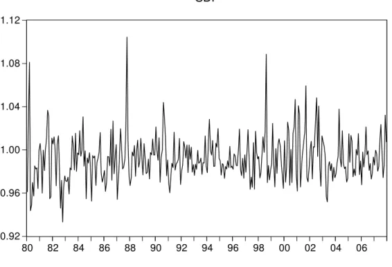
through 2007:12 (T = 336 observations), collected for N = 16;193 assets, grouped in the following four categories: mutual funds (7;932), stocks (6;009), real estate (383), and government bonds (1;869). After computingMct, we price individual return data not

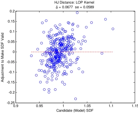
used in constructing it, measuring the distance between forecast prices and1 using the

pricing-error measure proposed in Hansen and Jagannathan (1997).

All return data used in this exercise come from CRSP. Mutual-Fund return data

comes from the CRSP Mutual Fund Database, which reports open-ended mutual-fund

returns using survivor-bias-free data. Bias can arise, for example, when a older fund

splits into other share classes, each new share class being permitted to inherit the entire

return/performance history of the older fund. Stock return data comes from the CRSP

U.S. Stock and CRSP U.S. Indices, which collects returns from NYSE, AMEX, NASDAQ,

and, more recently, NYSE Arca. Real-Estate return data comes from the CRSP/Ziman

Real Estate Data Series. It collects return data on real-estate investment trusts (REITs)

that have traded on the NYSE, AMEX and NASDAQ exchanges. Finally,

government-bond return data comes from CRSP Monthly Treasury U.S. Database, which collects

monthly returns of U.S. Treasury bonds with di¤erent maturities.

The …rst step to perform our exercise is computingMct. Since we do not have a random

sample of returns, we decided to work with each of the four categories above, weighting

them by their respective importance in the median U.S. household portfolio. For each of

the four asset categories (mutual funds, stocks, real estate, and government bonds) we

computed the geometric average of the reciprocal of all asset returns and the arithmetic

average of all asset returns. Based on the “Wealth and Asset Ownership” tables of 2004,

four categories as follows: Mutual Funds (10%), Stocks (10%), Real Estate (60%), and

Government Bonds (20%)11_{. They are a close approximation of the median (and also the}

mean) value of assets owned by U.S. households in these four categories. Local changes

in these weights (from5up to 20percentage points for individual categories) produce no

virtual change on the results of our exercise. Our …nal estimateMct results from weighting

geometric and arithmetic averages of returns in each of these four categories.

Once we obtain Mct, we forecast a group of returns not included in computing it for

all the 336 observations in the time-series dimension, comparing our results with unity.

Under the law of one price this exercise is similar in spirit to the one in Hansen and

Jagannathan (1997). Our forecasting exercise is performed using nominal returns either

in constructing the SDF or in out-of-sample evaluation of returns. Obviously, the product

MtRi;t is invariant to price in‡ation as long as the same price index is used in de‡ating

Mt and Ri;t.

Our estimate of Mt has a nominal mean of0:9922 in a monthly basis, which amounts

to 0:9106 in a yearly basis. In comparison, average yearly CPI in‡ation for the same period is3:85%. The plot of Mct follows below in Figure 2.

11_{These tables can be downloaded from http://www.census.gov/hhes/www/wealth/2004_tables.html.}

0.92 0.96 1.00 1.04 1.08 1.12

80 82 84 86 88 90 92 94 96 98 00 02 04 06

SDF

Figure 2: Stochastic Discount Factor

We want our forecasting exercise to be out of sample. In choosing the group of assets

which will have their returns priced, we require that they have not been included in

com-putingMct. To cover a wide spectrum of assets to be priced, we chose to work with stocks,

divided in 10 categories of capitalization, according to the CRSP Stock File

Capitaliza-tion Decile Indices. Their returns are calculated for each of the Stock File Indices market

groups. All securities, excluding ADRs on a given exchange or combination of exchanges,

are ranked according to capitalization and then divided into ten equal parts, each

rebal-ancing every year using the security market capitalization at the end of the previous year

to rank securities. The largest securities are placed in portfolio 10 and the smallest in

portfolio 1. Value-Weighted Index Returns including all dividends are calculated on each

of the ten portfolios. Because of the value-weighted character of these portfolios, and the

fact that they are rebalanced every year, their returns cannot be written as a …xed-weight