How much debtors' punishment?

No _{615 ISSN 0104-8910}

How much debtors’ punishment?

Aloisio Pessoa de Ara ´ujo, Bruno Funchal

Os artigos publicados são de inteira responsabilidade de seus autores. As opiniões

neles emitidas não exprimem, necessariamente, o ponto de vista da Fundação

How much debtors’ punishment?

Aloisio Araujo (IMPA and EPGE/FGV)

Bruno Funchal (EPGE/FGV)

Abstract

This paper investigates how the bankruptcy exemptions applied by the Personal Bank-ruptcy Law in each American state a¤ect the aggregated level of individuals and small businesses’ loans. Higher levels of bankruptcy exemptions imply in a lenient rule, mo-tivating debtors to …le for bankruptcy, what makes lenders worsen the terms of credit. On the other hand, lower levels of exemptions imply in a harsh punishment to debtors, inhibiting their demand for credit fearing a possible bankruptcy by bad luck. Con…rming the theoretical claims, empirical tests show the existence of a non-monotonic shape in the relationship between the bankruptcy exemptions and the amount of credit to individuals and small businesses, where the optimal level of exemptions should be neither too high nor too low. Since the majority of the states in U.S. do not apply the optimal level, an intervention that brings the exemption level closer to the optimal one can be credit and welfare enhancing.

Keywords: Personal Bankruptcy, credit. JEL Codes: G33; H81.

1

Introduction

The present study analyzes how the punishment applied to debtors a¤ects the aggregated level of individuals and small businesses’ loans. To access this question we took advantage of the changes provided by the Personal Bankruptcy Reform Act of 1978.

Personal bankruptcy law became much more favorable to debtors following the passage of such Reform Act. Prior to 1978, bankruptcy exemptions that de…nes what debtors can hold after the bankruptcy procedure were speci…ed by states and usually tended to be very low. The Commission on the Bankruptcy Laws of the U.S. argued that a high and uniform bankruptcy exemption would be bene…cial to less-well-o¤ individuals. Due to harsh collection practices by creditors, debtors often found it di¢cult to recover from these setbacks and would su¤er further adverse consequences such as bad health, family strain, divorce, job loss and for small businesses’ owners di¢culty to re-start a new businesses, unless a generous exemption in bankruptcy left them with adequate assets for a "fresh start".

While the House adopted the Commission’s populist view, the Senate preferred to continue allowing the states to set their own bankruptcy exemptions. For such con‡icts between the House and the Senate the solution was to specify a uniform bankruptcy exemption1_{, allowing}

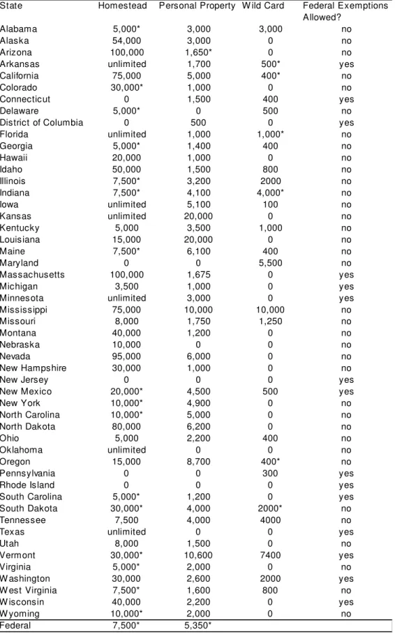
states to opt out of the federal exemption by adopting their own bankruptcy exemption. By 1983 all the states had done so, although one third of the states allowed debtors to choose between states and Federal bankruptcy exemptions. Many states raised signi…cantly their bankruptcy exemptions when they passed opt-out legislation, adopting widely varying exemption levels. In 1992 the lowest bankruptcy exemption level was in Maryland with no homestead exemption and USD 5,500 of personal bankruptcy exemption, while Texas’ exemption was unlimited for homestead and USD 30,000 for personal property.

Over the last years, a signi…cant number of individuals and small …rms …led for bankruptcy. In total, over the period 1992-2001, about 500,000 of small business and 11,194,000 of individuals …led for bankruptcy, what implies that for a ten years period more than nine percent of U.S. small …rms and four percent of individuals faced a bankruptcy …ling.

Individuals, ordinary and …rms’ owners, who …le for personal bankruptcy under Chapter 7 are required to give up all assets that exceeds the applicable state-speci…c exemption levels, but are not required to devote any of their future income to debt repayment. In return for giving up nonexempt assets, they receive a discharge from most types of debts. Thus, the exemption level can be seen as a debtors’ punishment variable that serves to protect creditors’ interests. The lower its level is, the harsher is the debtors’ punishment and the higher creditors’ protection is. Debtors are punished by losing a signi…cant amount of their wealth, and at the limit, when the exemption is zero, they lose everything they own. In this situation, fearing such harsh pun-ishment in bankruptcy states, debtors may avoid borrowing, diminishing the demand of credit. On the other hand, lower exemptions increase the amount that creditors receive from debtors in bankruptcy, making them more likely to supply credit. As the bankruptcy exemption rises, the punishment of the debtors falls since they still hold a good part of their wealth, making them more willing to …le for bankruptcy. Notice that bigger values of exemption make bank-ruptcy sates safer, motivating debtors to demand credit. But higher bankbank-ruptcy exemptions (or lower creditor protection) also reduce the amount that lenders receive in repayment of debt in bankruptcy states, making them more likely to refuse the credit o¤er.

Obseve that this legal instrument exerts an important in‡uence on incentives related to bankruptcy decisions, and ensuing on forces that drive the demand and the supply of loans.

Thus, this paper aims at answering the following issues: Is the relationship between debtors’ punishment (or creditors’ protection) and individuals and small businesses’ loans described by a non-monotonic shape? Is the optimal level of punishment intermediary? What is such an optimal level (in monetary terms)?

To reach our goals, …rst we present a theoretical approach that supports our empirical claims. Our model re‡ects certain features observed in the U.S. economy such as the possi-bility of debtors to …le for bankruptcy strategically or by bad fortune and the exemption level exogenously imposed by the bankruptcy law. Then, we simulate the model to analyze how the bankruptcy exemption a¤ects the welfare and credit market. Finally, we estimate an economet-ric model of the e¤ect of bankruptcy exemptions - that is the variable representing the debtors’

1_{USD 7,500 for homestead exemption, USD 4000 for personal property exemption, doubling when married}

punishment (or creditors’ protection) - on the equilibrium level of individuals and small busi-nesses’ credit in the economy using aggregated data of loans and information on bankruptcy exemption in each state over the period 1992-1997, when several changes occurred on exemption levels. Our estimate bene…ts from the Act of 1978 that changed the Personal Bankruptcy Law, allowing the states to choose their own bankruptcy exemption level.

We found a non-monotonic shape in the relationship between the bankruptcy exemption level and the amount of credit to both small businesses and individuals, as well the welfare. States with extreme levels of exemptions (high or low) tend to have a lower volume of credit relative to states with intermediary values bankruptcy exemptions. Thus, the punishment applied by the bankruptcy legislation should be neither so harsh that inhibits credit demand nor so lenient that worsen the credit o¤er conditions. This result suggests that an intervention on bankruptcy exemption levels can be good for the credit market and welfare.

The remainder of the article is organized as follows: section 2 discusses the literature review; section 3 discusses the personal bankruptcy law; section 4 presents the theoretical model; section 5 presents the empirical results; and section 6 concludes.

2

Literature Review

The literature on personal bankruptcy had its primary focus on the e¤ect of the personal bankruptcy reform of 1978 on the number of …lings in the course of time. Shepard (1984), Peterson and Aoki (1984), and Boyes and Faith (1986) found evidence that the bankruptcy reform of 78 increased the number of bankruptcy …lings relative to the period prior to 1978, but Domowitz and Eovaldi (1993) …nd that the reform was not signi…cant at all. White (1987) found that the number of Chapter 7 bankruptcy …lings in 1981 was positively correlated with the level of the state bankruptcy exemption.

Two articles examines empirically the e¤ect of personal bankruptcy law on business credit market. Scott and Smith (1986) studied the e¤ect of the new U.S. Bankruptcy Code, adopted in 1978, on business credit-market. They found empirically that adoption of the code caused the cost of business loans to increase and that lenders raised interest rates in response. Berkowitz and White (2004) uses cross-section variation in bankruptcy exemption levels across U.S. states to examine whether the exemption level a¤ect the supply of credit for small business.

In relation to the e¤ects of personal bankruptcy law on individuals’ credit, Gropp, Scholz and White (1997) investigated how varying bankruptcy exemption levels within the states af-fect markets for individuals’ loans. They found that in states with higher exemption levels, applicants are more likely to be turned down for credit but demand for loans increases.

Our study, in contrast, uses a pooled cross-section method to examine how the bankruptcy exemption levels a¤ect the volume of individuals and small businesses’ credit (the equilibrium level between supply and demand), trying to …nd out what is the optimal level of exemption to the economic environment.

that more creditor protection and better information sharing are associated with broader credit market. Contrary from the authors cited above, our paper shows that the relationship between creditors’ protection and volume of credit negotiated in the economy is not always increasing.

On the theoretical …eld, there is a large literature on credit markets with asymmetric in-formation that explores when credit rationing occurs, how it is reduced by borrowers pledging collateral, and whether low or high-risk borrowers are a¤ected when credit rationing occurs. However, the theoretical motivation of this paper comes from Dubey, Geanakoplos and Shubik (2005) who built a general equilibrium model that explicitly allows the possibility of default. Their idea is to impose on the agents a penalty for default. The authors show that in presence of incomplete markets, assuming that certain contingencies cannot be written into contracts, the intermediate level of penalty that encourages some amount of bankruptcy provides a higher level of individuals’ credit and welfare in the economy. Our paper approaches the debtors’ problem using similar features like incomplete markets and the imposition of exogenous debtors penalty. In our model the bankruptcy exemption is the exogenous penalty imposed to debtors in case of bankruptcy. Our results converge to Dubey, Geanakoplos and Shubik (2005) …ndings.

3

Personal Bankruptcy Law

The personal bankruptcy procedures apply directly to individuals and small businesses. The reason of why the personal bankruptcy law applies to small business, and not just to individuals, is because when a …rm is noncorporate, its debts are personal liabilities of the …rm’s owner, so that lending to the …rm is legally equivalent to lend to the owner. If the …rm fails, the owner can …le for bankruptcy and her business and unsecured personal debts will be discharged. When a …rm is a corporation, limited liability implies that the owner is not legally responsible for the …rm’s debts. However, lenders may require that the owner guarantee the loan with some personal good (second mortgage for example). Thus, personal bankruptcy law applies to noncorporate businesses and may also apply to small corporate business.

When individuals and unincorporated …rms2 _{…le under Chapter 7 of the U.S. Bankruptcy}

Code, they receive a discharge from unsecured personal and business debt in return for giving up assets in excess of the relevant state’s bankruptcy exemption. Creditors may not enforce claims against debtors’ assets if the assets are covered by Chapter 7 bankruptcy exemption and legal actions to obtain repayment. This provision prevents creditors from taking a blanket security interest in all debtors’ possessions.

While bankruptcy is a matter of federal law and the procedure is uniform across the country, Congress gave the states the right to set their own bankruptcy exemption levels, and they vary widely. Most states have several types of exemptions like residence exemption (homestead exemption), personal propriety exemption (like equity in cars, furniture, jewelry and cash) and wild card (where the debtor chooses anything to be exempted until some …xed value). Usually, the homestead exemption is the largest, and other exemptions are small.

There is also a second bankruptcy procedure, called Chapter 13, and debtors are allowed to choose between them. Under Chapter 13, debtors must present a plan to use some of their future earnings to repay part or their total debt, but all their assets are exempt. Debtors generally have an incentive to choose Chapter 7 rather than Chapter 13 whenever their assets are less than bankruptcy exemptions, because doing so allows them to avoid repayment debt

from either assets or future income. Because many states’ exemption levels are high relative to the assets of typical person who …le for bankruptcy, around 70 percent of all bankruptcy …lings occur under Chapter 73_{. Even when debtors …le under Chapter 13, the amount that they are}

willing to repay is strongly a¤ected by Chapter 7 bankruptcy exemption. Suppose, for example, that a person with assets of $50,000 living in a state whose exemption level is $35,000 considers …ling for bankruptcy. Because the debtor would have to give up $15,000 in assets if she …led under Chapter 7, she would be willing to pay no more than $15,000 (in present value) from future income if she …led under Chapter 13. As a result of this close relationship between both chapters, we ignore the distinction between them.

In 2005 a new bankruptcy law was adopted. Now, debtors must pass a series of means tests in order to …le for bankruptcy under Chapter 7. If debtors’ household income is bigger than the median level in their state and if their disposable income over a …ve-year period exceeds either $10,000 or 25% of their unsecured debt, then they must …le for bankruptcy under Chapter 13 rather than Chapter 7. In addition, the homestead exemption is limited to $125,000 unless debtors have owned their homes for 3 years and four months at the time they …le for bankruptcy4_.

But the reform seems unlikely to substantially reduce the overall number of bankruptcy …lings, since most debtors who …le for personal bankruptcy are in the lower half of the household income distribution in their states. Also, a sizable minority of Chapter 7 debtors could make a signi…cant contribution toward repayment of their non-housing debt over a …ve-year period. In particular, even assuming that all debtors are at the top half of the household income distribution in their states, approximately just 25% of Chapter 7 debtors declared income su¢cient to repay at least 30 percent of their nonhousing debt over 5 years while still maintaining their mortgage or rental payments on their homes, and just 20 percent have disposable income that overcomes $2,000 annually5_.

Now consider the set of small but incorporated …rms. Corporate …rms are legally separated from their owners, so owners are not personally responsible for debts of their corporations. Hold-ing everythHold-ing constant, this means that small corporations are less creditworthy than small unincorporated …rms, because the former have only the corporations assets to back up business debt, while the latter have both the …rm’s assets and the owner’s personal assets. Lenders also know that owners of small corporations can easily shift assets between their personal accounts and their corporations accounts, so that lenders may not view the corporation/noncorporation distinction as meaningful for small …rms. In making loans to small corporations, lenders there-fore may require that owners personally guarantee the loans. This abolishes the legal distinction between corporation and their owners for purposes of the particular loan and puts the owner’s personal assets at risk to repay the loan.

Debts can be divided into two di¤erent categories: secured and unsecured loans. Unsecured debts would seem more likely to be a¤ected by bankruptcy exemption than secured debts. In particular, this distinction is blurred and debtors are often able to arbitrage assets and debts across categories and thereby increase their …nancial bene…t from bankruptcy. For example, debtors might borrow on their credit cards or obtain new consumer loans in order to reduce secured credit. These transactions convert nondischargeable secured debt into unsecured debt that is dischargeable in bankruptcy. Or debtors might sell personal property that is in excess

3_{See Barron and Staten (1997)} 4_{See White (2005)}

of the personal property exempt and use the proceeds to reduce their mortgage or to buy exempted property. In addition, bankruptcy undermines the value of collateral to lenders, since lenders may be delayed in repossessing it or may be unable to repossess the collateral at all (for example, if they call to repossess an asset that they do not provide money to …nance its purchase)6_{. Also, lenders incur extra legal costs because they must obtain the permission of the}

bankruptcy trustee in order to repossess collateal. For these reasons we examine the e¤ects of bankruptcy exemptions on total loans rather than on unsecured loans.

4

Theory

In this section we build a model that describes how the debtors’ decision for bankruptcy develops, considering the di¤erent levels of punishment provided by the value of the bankruptcy exemption imposed by the local law. We present in the …rst part the case for individuals, and in the second part the case for small businesses.

4.1

Individuals’ Model

Consider a consumer who lives for two periods and maximizes utility over her consumption c:

The consumer born with some amount of durable goods of value D (like a house, a car, etc) that she consumes in both periods, but it depreciates at rate :Period 1 incomew1 is observed

but the second period income is uncertain, varying according to the realization of the states of nature, thus w2s 2 [w21; w2S]: Each state occurs with probability ps, where ps > 0 8s and

X

s

ps = 1:The wage is free observed by the borrower, but the lender may verify its value at a

monitoring cost proportional to the borrowed amount B: The monitoring cost will be denoted by B:

There is a large number of agents divided in two di¤erent groups: borrowers and lenders. Borrowers may be thought as consumers and lenders as the …nancial institution. Each lender is endowed with enough money to supply credit to consumers. Such lenders’ endowment may be used either to lend to a borrower with rate r; or to purchase a risky-free asset paying an exogenously given rate of returnrf:

If the borrowers report bankruptcy, part of the debt will be discharged, and some of the individuals’ assets, including personal goods (D) and their present income will be exempted up to the amount E: The bankruptcy law determines the level of E exogenously, and accordingly we call E the bankruptcy exemption level in this paper. The debt contract is subject to this bankruptcy law. Notice that part of borrowers’ goods serves as an informal collateral imposed by the law to unsecured credit.

De…nition 1 Strategic bankruptcy7_{: It occurs when the borrower has enough wealth to pay her}

debts but she chooses not to do it.

6_{In relation to debtors’ home, they may be able to get rid of some lien (junior creditors, like second mortgages)}

without paying a cent to the lienholder. In some states, if debtors’ home is sold in bankruptcy, they will get their homestead amount ahead of junior secured creditors holding judicial liens. Debtors can get rid of the lien created by judgment by …ling a "motion to avoid a judicial lien". They may also be able to get rid of some liens by …ling separate lawsuit in bankruptcy court. See Elias, Renauer, Leonard and Michon (2004)

De…nition 2 Bankruptcy by bad fortune: It occurs when the realization of states of nature is bad in such way that borrowers are unable to ful…ll their repayment promises.

The consumption of the …rst period de…nes the level of debtB at the beginning of period 2:

B = (c1 D w1);

which means that the agent consumes more than the sum of her wage and durable goods. A loan contract between the borrower and the lender consists of a pair (r; B); where B is the loan volume and (1 + r) the loan rate, subject to the legal imposition on the exemption level E that applies to the situation in which the borrower does not repay the debt (1 +r)B.

If at least some debt will be held, so that B > 0, we can divide the borrowers’ actions in three distinct choices:

C1 does not …le for bankruptcy if: w2s+ D (1 +r)B and(1 +r)B max(w2s+ D E;0)

C2 strategic bankruptcy if: w2s+ D (1 +r)B and (1 +r)B >max(w2s+ D E;0)

C3 bad fortune bankruptcy if: w2s+ D <(1 +r)B (and therefore(1 +r)B >max(w2s+ D

E;0))

Analyzing the consumer choice for bankruptcy, it is optimal to …le for bankruptcy if and only if their gains in bankruptcy are bigger than their gains when they choose not to …le for bankruptcy, i.e., if and only if(1+r)B >max(w2s+ D E;0):That is, the consumer will default

whenever the second period debt exceeds the level of assets that can be seized and the debt can not be fully enforced. Therefore the consumer deliverymin[(1+r)B;max(w2s+ D E;0)]:This

way, we can view the probability of no bankruptcy as(1 pbankruptcy) = p(C1) =

X

s

ps s(1 d)

and the probability of bankruptcy aspbankruptcy =p(C2)+p(C3) =

X

s

ps[ s d+ (1 s)];where

s= 1 if w2s+ D (1 +r)B and d= 1 if (1 +r)B >max(w2s+ D E;0):

The wealth in each situation for the borrowers is given as follows:

W2 =

w2+ D (1 +r)B if no bankruptcy

w2+ D max(w2s+ D E;0) if bankruptcy

Thus the lender can receive in case of bankruptcy a payment between w2s + D (if the

bankruptcy exemption is zero) and zero (if the bankruptcy exemption overcomes the debtors’ wealth in the second period).

For the lenders, the expected return on lending must be no less than the risk-free return. Therefore, the lender’s participation constraint is:

(1 +rf)B

X

s

ps s(1 d)(1 +r)B+ (1)

+X

s

ps[ s d+ (1 s)] [max(w2s+ D E;0) B] ;

The extra interest rate paid r rf is exactly the one needed to o¤set the loss the …nancial

For a menu of the described contracts, the consumer chooses a pair (r; B) that maximizes her expected utility function.

max

(r;B)Eu(c) =u(c1) +

" _S X

s=1

psu(c2s)

#

st (1) and

c1=w1 +D+B

c2s=w2s+ D min[(1 +r)B;max(w2s+ D E;0)] 8s

The constraint (1) is always valid with equality, since a smaller rate of return r makes the borrower strictly better and still makes the lender’s participation constraint valid. Also, since the lender pays the monitoring cost to verify the wage value (w) in default states, the contract speci…ed above is incentive-compatible in the sense that borrowers do not have incentive in declaring a false state of nature.

Observe that the lenders’ expected return, described by their participation constraint, de-termines the supply of credit in the economy. The supply of credit depends directly on the bankruptcy exemption level imposed by the local legislation. Intuitively, as E approaches to the unlimited level, the number of the states of nature in which the borrower does not default reduces, since the bigger the exemption level is, the lower is the possibility that the income value plus borrower’s goods overcome the exemption level, increasing the possibility of strategic bankruptcy. Such excess of strategic bankruptcy increases the interest rate charged to the loans, and at the limit, the borrower has incentive to …le for strategic bankruptcy in every state and the supply of credit goes to zero. On the other hand, ifE goes to zero, i.e. there is no exemption for borrowers, it rules out the strategic bankruptcy and increases the seizure of debtors’ goods, raising the possibility of ful…llment of debtors’ payment promises and consequently diminishing the cost of credit (r).

Proposition 1 Any value of exemptions above the critical value E* makes the supply of credit

to individuals zero.

Proof. See Appendix A.

Proposition 2 As the bankruptcy exemption decreases, the interest rate charged to individuals

reduces.

Proof. See Appendix A.

Proposition 3 As the bankruptcy exemption rises, the individuals’ demand for credit increases.

Proof. See Appendix A.

Therefore, there are two distinct forces acting in the proposed problem. If E decreases, the supply of credit is motivated, reducing the interest rate charged to borrowers, since the chances of creditors being repaid are bigger. On the other hand, the demand is repressed since the debtors fear the punishment for losing their goods. With an increase of E there is an incentive to consumers demand credit since they can keep a bigger amount of their personal goods if bankruptcy occurs, making such state of nature safer. On the other hand, such level of exemption inhibits the lenders’ supply of credit since the chance and the amount of repayment fall.

Thus, there is a trade-o¤ that concerns the choice of the exemption level: higher levels of exemption increase the demand of credit but also stimulate the moral hazard problem, lowering the supply of credit; on the other hand, lower levels of exemptions mitigate the moral hazard problem - what motivates the supply of credit - but this also has a negative e¤ect on the demand side due to the fear of harsh punishment. The equilibrium level of credit provided by extreme levels of bankruptcy exemption (0 or unlimited) tends to be very low or even zero. An optimal level of bankruptcy exemption E may exist where the the equilibrium of supply and demand of credit provide a higher level of credit and welfare in the economy.

The Simulation of the Equilibrium

Through the simulation method we intend to show how the equilibrium values of credit and welfare change as the bankruptcy exemption varies.

To simulate the model we simplify the setup described before. Now, the model has two periods, two states of nature in the second period (s=H; L) and two types of agents (lenders and borrowers). The lenders are risk-neutral and the consumers are risk-averse with logarithm utility function.

The debtors’ problem is:

max

r;B Eu(c) = ln(c1) + [pLln(c2L) +pHln(c2H)]

st(1);and

c1 =w1 +D+B

cL =w2L+ D min[(1 +r)B;max(w2L+ D E;0)]

cH =w2H + D min[(1 +r)B;max(w2H + D E;0)]

The model simulation will be done according to the following value of parameters: w1 =

0:5; w2H = 1:5; w2L = 0:5; D = 0:3; = 0:9; pH =pL = 0:5; = 0:95; = 0:01 andrf = 1:05: We

can interpret such wage values as the one of a person who is employed receiving 0.5 and expects a promotion for a better job that pays 1.5. The promotion occurs with probability of 0.5. Only the parameter E will be varying.

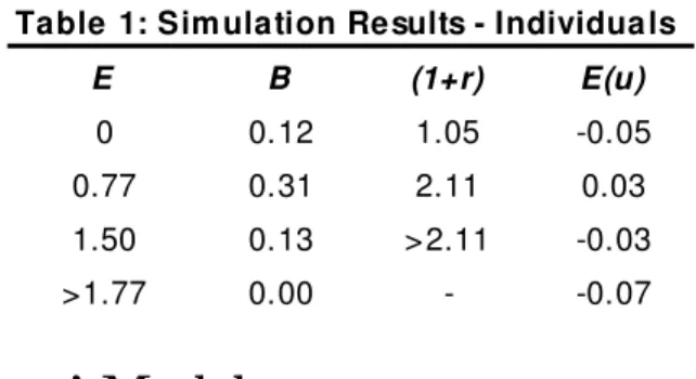
to have some amount of their goods if bad state of nature occurs makes them more willing to demand credit, even paying higher interest rates. This result is very intuitive because for risk-averse individuals, a moderate exemption level works as a security against bad realizations, where the cost of this security is the di¤erence between the current and the former interest rates. Increasing even more the exemption level, the welfare and the volume of credit decrease - considering that the supply is inhibited due to the major possibilities of strategic bankruptcy - and the interest rates charged to individuals increases (see proposition 1 and 2). Thus, the volume of equilibrium of the creditB is a non-monotonic function of the bankruptcy exemption levels E; where the optimal level of exemption is intermediary, providing a punishment neither too harsh nor too lenient.

Table 1: Sim ulation Results - Individua ls

E B (1+r) E(u)

0 0.12 1.05 -0.05 0.77 0.31 2.11 0.03 1.50 0.13 >2.11 -0.03 >1.77 0.00 - -0.07

4.2

Small Businesses’ Model

Now, there is only one time period, where the small …rms’ owners choose the necessary amount of capital B to invest in their investment project. Then, a random amount of output is produced by the borrower’s project. Finally, the payment speci…ed by contract and the consumption occur.

Each investment project requires capital as input to begin its operation, then it produces a random amount wB , where w is the random variable, B is the amount that was borrowed and invested in the project. The output, that is uncertain, varies according to the realization of the states of nature ws 2[w1; wS]: Each state occurs with probability ps, where ps >0 8s and

X

s

ps = 1: As before, the project return is free observed by the borrower, but the lender may

verify the return at a monitoring cost proportional to the borrowed amount B:The monitoring cost will be denoted by B:

There is a large number of agents divided in two di¤erent groups: borrowers and lenders. Here, borrowers may be thought of as entrepreneurs of small …rms. Lenders and borrowers di¤er in their preferences, their access to capital, and their access to the investment technology. Each lender is endowed with the capital input that can be used to put the entrepreneur’s project in operation. If it happens, they lend their capital to the borrowers with rate r; otherwise they purchase a risky-free asset paying an exogenously given rate of return rf: Each borrower

is endowed with an investment project, but none of the capital input required to operate the project initially. Also borrowers own an amount of tangible goods denoted by D that can not be used as capital input.

If at least some debt will be held by the …rms’ owners, so that B > 0, we can divide their actions in three distinct choices:

C1 does not …le for bankruptcy if: wsB +D (1 +r)B and(1 +r)B max(wsB +D E;0)

C2 strategic bankruptcy if: wsB +D (1 +r)B and (1 +r)B >max(wsB +D E;0)

C3 bad fortune bankruptcy if: wsB +D <(1 +r)B:

Thus, the lender’s participation constraint is:

(1 +rf)B

X

s

ps s(1 d)(1 +r)B + (2)

+X

s

ps[ s d+ (1 s)] [max(wsB +D E;0) B] ;

where s = 1 if wsB +D (1 +r)B and d= 1 if (1 +r)B >max(wsB +D E;0):

For a menu of the described contracts, the entrepreneur chooses a pair(r; B)that maximizes his expected utility function.

max

(r;Bl)Eu(cs) = S

X

s=1

psu(cs)

st (2) and

cs =wsB +D min[(1 +r)B;max(wsB +D E;0)] 8s (3)

The constraint (2) is always valid with equality, since a smaller rate of return r makes the borrower strictly better and still makes valid the lender’s participation constraint. Since the lender pays the monitoring cost to verify the productivity (w) in default states, the contract speci…ed above is incentive-compatible in the sense that borrowers do not have incentive in declaring a false state of nature.

The supply of credit, which is described by the lenders’ participation constraint, depends directly from the exemption level imposed by local legislation. The intuition of individuals’ case works perfectly here, where the higher level of bankruptcy exemption acts to increase the number of states of nature that debtors …le for strategic default and to reduce the recovery of lenders in bankruptcy, increasing the interest rate charged by them. At the limit, the supply of credit disappears.

Proposition 4 Any value of exemptions above the critical value E* makes the supply of credit

to small businesses zero.

Proof. See Appendix A.

Proposition 5 As the bankruptcy exemption decreases, the interest rate charged to small

Proof. See Appendix A.

The bankruptcy exemption value also has a strong e¤ect on the entrepreneurs’ demand for credit. For higher levels of bankruptcy exemption, the entrepreneurs tend to keep a signi…cant part of their goods and gains from production, allowing a fresh re-start in case of bankruptcy and making more attractive the demand for credit. Conversely, for lower levels of bankruptcy exemptions the entrepreneurs may avoid demand for credit, fearing a bad realization of the states of nature. This happens because for w is su¢ciently low, the borrower does not have enough wealth to ful…ll the repayment promise, i.e. wB +D <(1 +r)B; leaving to the …rm’s owner a small amount (or even nothing) of her wealth, practically eliminating the possibility of a fresh re-start.

Proposition 6 As the bankruptcy exemption rises, the small businesses’ demand for credit

increases.

Proof. See Appendix A.

As the individuals’ problem, there are two distinct forces acting in this situation: the supply of credit that is boosted when E decreases and inhibited when it increases, and the demand of credit that has the inverse behavior. The existing trade-o¤ between strategic bankruptcy and the level of credit provide a non-monotonic shape in the relation between bankruptcy exemptions and small businesses’ credit and welfare. As we will see next, in equilibrium the level of credit provided by extreme levels of exemption (0 or 1) tends to be very low or even zero, while the maximal level of credit and welfare occurs when the level of bankruptcy exemption E is intermediary.

The Simulation of the Equilibrium

To simulate the model we made the same simpli…cations as the individuals’ case: two states of nature and two types of agents where lenders are neutral and entrepreneurs are risk-averse with logarithm utility function.

The entrepreneurs’ problem is:

max

r;B Elog(c) = pHlog(cH) +pLlog(cL)

st(2);and

cL =wLB +D min[(1 +r)B;max(wLB +D E;0)]

cH =wHB +D min[(1 +r)B;max(wHB +D E;0)]

The model simulation will be done according to the following value of parameters: = 0:3; D = 0:3; pH =pL = 0:5; wH = 1:5; wL = 0:5;(1 +rf) = 1:05 and = 0:01:Again, only the

parameter E will be varying.

Ta ble 2: Sim ula tion Re sults - Sm a ll Busine sse s

E B (1+r) E (u)

The same intuition used for individuals can be applied here. Simulation results tell us that lower levels of exemption inhibit the demand of credit, since the harsh punishment eliminates the possibility of fresh re-start, as the proposition 6 showed. As the exemption level increases, the amount of credit negotiated and welfare rise, reaching its maximal level. Even considering the increase in the interest rates, the possibility of entrepreneurs save some amount of their goods in case of bad state of nature make them more willing to demand credit, which raises their expected utility. It is very intuitive because for risk-averse entrepreneurs a moderate exemption level works as a security against bad realizations, which provides the possibility of a fresh re-start. Increasing even more the exemption level the welfare and the volume of credit decrease, once the terms of credit deteriorate due to the major possibilities of strategic bankruptcy. Thus, the equilibrium of the volume of credit B is a non-monotonic function of the exemption levels

E:

5

Empirical Tests

In this study we use data from 1992 to 1997 from the Federal Deposit Insurance Corporation

Statistics on Banking (FDIC) for small businesses and individuals’ loans in each U.S. state and

information on states’ bankruptcy exemption to examine the empirical hypothesis. Comparing each state, we have 51 observations for a cross-section analysis. Since several changes happened in the levels of bankruptcy exemptions (which determine the debtors’ punishment) during the period 1992-19978_{, we will test the relationship between the degree of punishment and the}

level of individuals and small businesses’ loans using a pooled cross-section method, raising the sample to 306 observations.

Most states have separate exemptions for equity in homesteads, personal property like equity in motor vehicles, some amount of cash, jewel, furniture, clothing etc, and miscellaneous category (wild card). Some states allow debtors to choose between the state’s exemption and the Federal exemption, and for empirical tests we will use the bigger one. Also, some states allow married couples who …le for bankruptcy to double (or raise) their exemptions. Because we are working with aggregated data, we assume that co-applicants are actually married couples9_{and we double}

(or otherwise raise) the exemptions in states that allow it. Table A in Appendix A lists the homestead, the personal property and the wild card exemptions in each state in 1992 and their changes until 1997. The table also indicates whether each state allows its residents to use Federal exemptions and whether it allows married couples to double the exemption.

The structure of the bankruptcy law and its reform in 1978 bene…ted our estimation in two di¤erent ways: the …rst is because inside the U.S. there is a well-controlled institutional environment where the only issue that distinguishes the bankruptcy procedure in the American states is the level of bankruptcy exemption, which varies widely across states; second is that the reform in the Personal Bankruptcy Law in 1978 provides a neat natural experiment.

To run our tests we construct a debtors’ punishment variable10_{. We can de…ne debtors’}

8_{See Table A in the appendix.}

9_{As in Lin & White (2001) and Berkowitz & White (2004). Usually, more than 70% of debtors are married}

(Sullivan (1982)).

10_{The option to use this variable instead of bankruptcy exemption was made because the bankruptcy exemption}

protection as a sum of homestead, personal property and wildcard exemption, that is how much cannot be taken o¤ from the debtor in case of bankruptcy11_{. Notice that this variable is}

inversely related to the penalty imposed on the debtors in their state, because the higher (lower) the debtor exemption, the less (more) the creditor can seize the debtors’s goods. So this variable can be seen as the inverse of debtors’ punishment. Normalizing the bankruptcy exemption by the lowest level and calculating its inverse, the variable used as the debtors’ penalty is:

Debtors’ Punishment = _{N ormalized Exemption}1 2[0;1]:

The measures of the aggregated level of equilibrium for individuals’ loans that we use to run the regressions are:

CCL=amount of credit card loans given by …nancial institutions to individuals divided by GSP,

P L = amount of personal loans12 _{given by …nancial institutions to individuals divided by}

GSP,

T IL = P L+CCL = total amount of loans given by …nancial institutions to individuals divided by GSP.

Concerning small businesses’ loans, the measures used to run the tests are:

SBL1 =amount of loans of $100,000 or less given by …nancial institutions to small business divided by GSP,

SBL2 =amount of loans between $100,000 and $250,000 given by …nancial institutions to small business divided by GSP,

SBL3 = amount of loans between $250,000 and $1,000,000 given by …nancial institutions to small business divided by GSP,

SBL= SBL1 +SBL2 +SBL3 = amount of loans given by …nancial institutions to small business divided by GSP.

To investigate the non-linear shape of the relationship between debtors’ punishment and each measure of loans we regress with and without state and year …xed e¤ects the logarithm13 of each measure of individuals and small businesses’ loans on the punishment variable, its square and other control variables.

To test our hypothesis, one possibility is to analyze whether di¤erences in punishment levels across states a¤ect the volume of credit. However, cross-section results are vulnerable to crit-icism because the punishment variables may be acting as proxies for nonbankruptcy variables

of the population. The debtors’ punishment variable works to full…l this feature.

11_{For states that have an unlimited exemption level, we decided to impose a level of $500,000 (quite above}

the highest level of exemption established by an American State, namely, $100,000). To check the robustness of this hypothesis tests were done with values of $250,000, $1,000,000 and1(debtors’ punishment equals zero) for unlimited bankruptcy exemptions. The regressions present only marginal changes compared with the last results and the variable of interest remains signi…cant in all cases.

12_{Other loans to individuals for household, family and other personal expenditures (consumer loans) including}

single payment, installment and all student loans. Included are loans for such purposes as: (1) purchases of private passenger automobiles, pickup trucks, household appliances, furniture, trailers, and boats; (2) repairs or improvements to the borrower’s residence (not secured by real estate); (3) educational expenses, including student loans; (4) medical expenses; (5) personal taxes; (6) vacations; (7) consolidation of personal (nonbusiness) debts; (8) purchases of real estate or mobile homes (not secured by real estate) to be used as a residence by the borrower’s family; and (9) other personal expenditures.

13_{Because the distribution of individuals and small businesses’ loans are right-skewed, we use the natural}

at the state level which are omitted from the regression. The usual response to this problem in the program evaluation literature has been to use pooled cross-section or panel data rather than single year cross-section data and to introduce both state and year …xed e¤ects14_{. Using}

pooled cross-section data and introducing state dummy variables into the estimation, the state dummies will capture the e¤ect of variation across states in the punishment levels, while the punishment variable themselves will capture only the e¤ects of changes in the punishment level between 1992 and 1997. We will report results using the following speci…cations:

ln(Lit) = + 1(punishmentit) + 2(punishmentit)2+ Xit+"it (4)

ln(Lit) = i+ t+ 1(punishmentit) + 2(punishmentit)2+ Xit+"it (5)

The same monetary penalty could vary with each person, and a monetary penalization could be stronger the less income the agent owns. Therefore, it is possible to de…ne a debtors’ punishment variable as the inverse of the sum of homestead, personal property and wildcard exemption weighing up for each state per capita income because, for example, an exemption of $10,000 in a rich state is a bigger penalty than the same exemption for a poor state. Let us call this variable as E¤ective Debtors’ Punishment15_{. Then, we re-estimate the equations (4) and}

(5) for all measures of loans replacing debtors’ punishment by e¤ective debtors’ punishment:

ln(Lit) = + 1(ef:punit) + 2(ef:punit)2+ Xit+"it (6)

ln(Lit) = i+ t+ 1(ef:punit) + 2(ef:punit)2+ Xit+"it: (7)

In the speci…cation without …x e¤ects the vector of control variables is composed by GSP (in logs), population (in logs), unemployment rate of previous year16, number of previous year of bankruptcy …lings17 _{per 1000 inhabitants or small businesses and dummies for American}

regions (Farwest is the excluded category)18_{. We control for total GSP on the theory that}

larger economies may have bigger credit markets because of economies of scale in organizing the supporting institutions. Inserting the population variable we also control by itself and for GSP per capita (log (GSP) - log (population) = GSP per capita). The inclusion of the variable number bankruptcy …lings in the area works to capture the strategic behavior of the local lending market. The state unemployment rate in the previous year controls for the labor market activity and for the potential bankruptcy by bad fortune. Finally, we use dummy variables for regions to account for potential geographic variation in credit markets. Except for the dummies for

14_{The state …xed e¤ects control for state-speci…c factors that are …xed over time, and the year …xed e¤ects}

control for factors that vary over time but are common accros all states.

15_{The range of this variable goes from zero to 5.5.}

16_{The data source of Gross State Product (GSP), population and unemployment rate is the U.S. Bureau of}

Economic Analysis.

17_{Source: www.uscourts.gov}

18_{The regions used as dummies are: Mideast, New England, Plains, Rocky Mountain, Southeast, Great Lakes,}

regions, we use the same controls in the …xed e¤ect speci…cation because there is some variation that is not state- and time-speci…c19_.

But there exists an important econometric question: should the exemption levels be endoge-nous? Exemption levels can be treated as exogenous to the development of the credit-market. The U.S. Congress adopted a new Bankruptcy Code in 1978 which speci…ed uniform federal bankruptcy exemptions that were applicable all over the United States, but also allowing states to opt out of the federal exemption by adopting their own bankruptcy exemption. The code went into e¤ect in late 1979, and all the states adopted their own bankruptcy exemptions within a couple of years thereafter, although about one-third of the states allowed their residents to choose between the state’s exemption and the federal exemption. Since the early 80s, the pat-tern has been that only a few states changed their exemption levels each year, mainly to correct nominal exemption levels for in‡ation. From 1992 to 1997, states changed their homestead exemptions 11 times and changed their personal property exemptions 10 times. Many of these changes were very small. In addition, the Federal bankruptcy exemption was raised in 1994 and this raised exemption levels in six states that allow their residents to use the Federal exemption. The fact that most states adopted their bankruptcy exemptions within a short period after the code went into e¤ect and that few states changed their exemption levels each year suggests that individual states’ bankruptcy exemptions can be treated as exogenous to the state credit market behavior.

5.1

Tests for Individuals’ loans

Table 3 reports the coe¢cient values of running an ordinary least-squares, with and without state and years …xed e¤ects, aiming at explaining the relationship between individuals’ loans and debtors’ punishment. For all types of loans (personal loans, credit card loans and total individuals’ loans) and econometric speci…cations the coe¢cients describing debtors’ punishment are highly signi…cant, and since the …rst coe¢cient is positive and the second is negative, the relationship has a concave form.

Figure 1 (T ILwith region dummies) that illustrates the non-monotonic shape of the studied relation shows that there is an intermediary penalty that is optimal for the development of the states credit market. Similar shapes hold for the other two measures of individuals’ credit: credit card loans and personal loans.

Notice that as we claim in the theoretical section, there is an intermediary level of debtors’ punishment - and consequently of bankruptcy exemption - that maximizes the level of indi-viduals’ credit negotiated in the economy. For lower levels of punishment (higher exemptions) the terms of credit o¤ered by the lenders tend to worsen, diminishing the supply of credit and increasing the interest rate since the possibility of strategic bankruptcy by the borrowers is higher (proposition 1 and 2), generating a low level of credit negotiated in the economy. As the punishment increases, the incentive to …le for bankruptcy declines, improving the terms of credit and the equilibrium level of credit. However, if the punishment increases too much, the demand for credit is inhibited since the debtors fear the consequences of bankruptcy (proposition 3), reducing again the amount of individuals’ loans. Therefore, there is an intermediary level that

19_{We also run the regressions without the controls, only with the …xed e¤ects. The varibles of interest present}

is optimal for the credit market which maximizes the amount of individuals’ credit.

Dependent variable

constant _-10.20a

62.00a -4.75b -2.18 -5.80a 6.51 (0.75) (19.11) (2.11) (35.08) (1.34) (23.47)

Debtors' Punishment _1.78a

3.99a 5.20a 5.67c 3.21a 3.35b (0.36) (1.12) (1.15) (2.95) (0.67) (1.56)

Debtors' Punishment^2 _-2.09a

-6.48a -5.45a -13.06b -3.57a -8.04b (0.44) (1.84) (1.47) (5.84) (0.82) (3.19)

ln(GSP) _-2.00a _1.25

-1.09a 1.98 -1.88a 2.13 (0.15) (1.12) (0.41) (2.39) (0.26) (1.36)

ln(population) _1.99a

-5.91a 0.99b -1.70 1.71a -2.30 (0.15) (2.01) (0.42) (3.66) (0.27) (2.42)

unemployment(-1) _-0.09a

-0.10a -0.36a -0.14c -0.22a -0.11a (0.02) (0.03) (0.05) (0.08) (0.04) (0.04)

Fixed Effects No Yes No Yes No Yes

Dummies of regions Yes No Yes No Yes No

R-square 0.56 0.82 0.23 0.85 0.35 0.87

Note: Standard errors and covariance robust to heteroskedasticity. Standart errors are in parentheses.

a-significant at 1%, b-significant at 5%, c-significant at 10%.

TIL CCL

PL

Table 3: OLS Regression - pooled cross-section with 306 observations

Figure 1: Debtors’ Punishment x Total Individuals’ Loans/GSP

-0,8 -0,6 -0,4 -0,2 0 0,2 0,4

0 0,1 0,2 0,3 0,4 0,5 0,6

Debtors' Punishment

T

ot

al

I

nd

iv

id

ua

ls

'

Lo

a

ns/

G

S

P

Con…dence Interval: optimal level of punishment and exemption

90% 95%

debtors0 _{punishment (0:192; 0:223) (0:188; 0:226)} bankruptcy exemption($24;663; $28;645) ($24;336; $29;255)

Moreover, since the bankruptcy exemption is a function of debtors’ punishment, we can calculate the con…dence intervals for the levels of bankruptcy exemptions that provide the maximal level of individuals’ credit.

We can say with 90% of con…dence that the optimal bankruptcy exemption level for an American state that maximizes total individuals’ credit in the economy belongs to the interval

($24;663; $28;645). Observe that it is not optimal for the economy a punishment to be neither su¢ciently harsh nor su¢ciently lenient.

Dependent variable

constant _-10.22a

64.33a -5.08b 12.26 -5.94a 11.13 (0.76) (18.97) (2.09) (35.84) (1.34) (23.78)

Ef. Debtors' Punishment _0.36a

0.64a 1.17a 1.41a 0.69a 0.52a (0.07) (0.16) (0.23) (0.41) (0.13) (0.20)

Ef. Debtors' Punishment^2 _-0.09a

-0.12a -0.27a -0.49a -0.17a -0.17a (0.02) (0.03) (0.06) (0.08) (0.03) (0.04)

ln(GSP) _-2.04a _1.33

-1.29a 2.19 -1.99a 2.34c (0.15) (1.12) (0.42) (2.32) (0.27) (1.34)

ln(population) _2.03a

-6.14a 1.16a -2.97 1.80a -2.81 (0.16) (2.00) (0.43) (3.64) (0.28) (2.41)

unemployment(-1) _-0.10a

-0.10a -0.36a -0.14c -0.22a -0.11a (0.02) (0.03) (0.06) (0.08) (0.04) (0.04)

Fixed Effects No Yes No Yes No Yes

Dummies of regions Yes No Yes No Yes No

R-square 0.56 0.83 0.24 0.86 0.35 0.87

Note: Standard errors and covariance robust to heteroskedasticity. standart errors are in parentheses

a-significant at 1%, b-significant at 5%, c-significant at 10%

TIL CCL

PL

Table 4: OLS Regression - pooled cross-section with 306 observations

In 1992, only eight states in the U.S. apply bankruptcy exemptions that are within the optimal range, while twenty-…ve apply exemptions above this range and eighteen below it. Until 1997 the set of states with exemptions above the optimal range increases dramatically to thirty-four, while the number states with exemptions within and below the optimal range falls to two and …fteen respectively. Moreover, the most signi…cant feature is that there are several states that apply extremely high exemptions, what diverges from its primary objective that was to bene…t the less-well-o¤ individuals20_{. In this case the state is protecting everybody too much,}

including those who have a signi…cant amount of wealth and who are able to repay their debts, giving a strong incentive to …le for bankruptcy.

It is observable that between 1991 and 1998 the median net value of holdings21 _{of an}

individ-ual ‡uctuates within a fairly narrow range from 40,000 to 46,000 dollars22_{. Applying the optimal}

exemption it is possible to provide both a fresh start to failed debtors - since they will still hold approximately between $24,000 - $29,000 dollars of their goods - and a signi…cant recovery to lenders (11,000 dollars at least) since the median amount of debts that …le for Chapter 7 bank-ruptcy is approximately 32,000 dollars23 _{(more than 34% of the debt). However, because of the}

higher levels of exemptions in most states what really happens is that debtors are motivated to …le strategically for default, and creditors do not receive a signi…cant amount of the debt (in 20 states the bankruptcy exemption is bigger than the median value of holdings).

To exemplify the e¤ect of the optimal bankruptcy exemption on individuals’ credit, suppose that a state that applies a bankruptcy exemption of 200,000 dollars (like Minnesota in 1997) decides to modify its bankruptcy exemption to the optimal level (approximately 26,500). Such a change, according to the regression results, tends to produce an increase of 30% in the level of credit, raising the level of individuals’ loans/GSP from 0.0975 to 0.127. Conversely, states with too low exemptions, like Nebraska with a bankruptcy exemption of 12,500 dollars, produces an increase of almost 54% raising the measure of individuals’ credit from 0.1024 _{to 0.154.}

Since the reaction of the credit market to debtors’ punishment was estimated, we can calcu-late the potential e¤ect of the upper bound of $125,000 for the homestead exemption imposed by the new personal bankruptcy law. Seven states are a¤ected by this new feature: Arkansas, Florida, Iowa, Kansas, Minnesota, Oklahoma and Texas. Except for Minnesota ($200,000 of homestead exemption), the rest apply the unlimited value. The change in the law may produce approximately an increase of 4.5% and 10% in the level of personal credit in Minnesota and the others states with unlimited value respectively.

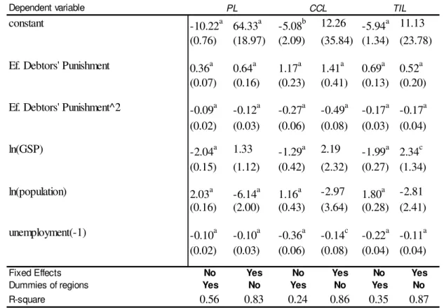
Running the same test for e¤ective debtors’ punishment, table 4 shows that the results are again highly signi…cant, independent of the speci…cation. For the three measures of individuals’ loans, the result of intermediary optimal level of debtors’ punishment still holds, meaning that even considering the penalty as a portion of individuals’ income (a real variable instead of a nominal variable) our claim is also valid.

5.2

Tests for Small Businesses’ loans

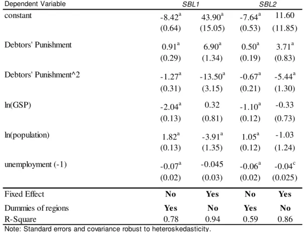
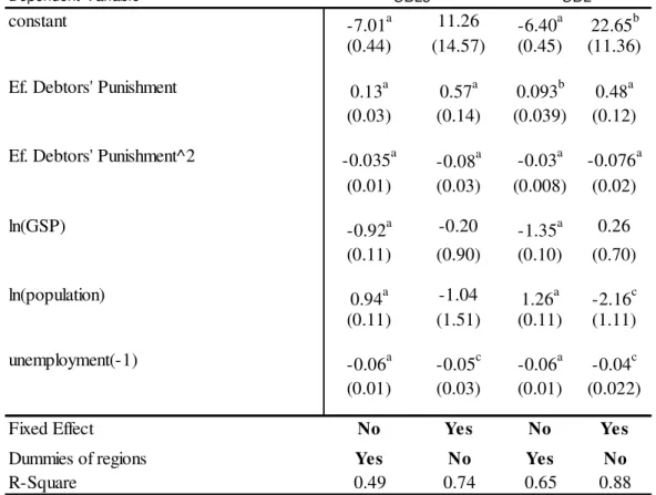
Table 5 reports the results of running a OLS regressions explaining how the debtors’ punishment a¤ects small business’ credit. The SBL1 columns report the regression when the dependent variable is loans under $100,000, the SBL2 and SBL3 columns report results for loans between $100,000 and $250,000, and $250,000 and $1,000,000 respectively. Finally the SBL columns report the total amount of loans to small businesses.

The coe¢cients describing debtors’ punishment are signi…cant at the 99% level in all cases, and since the …rst coe¢cient is positive and the second is negative, the relationship has a concave form. Moreover, since the debtors’ punishment varies in an interval between 0 and 1, there is an intermediary punishment that maximizes the volume of loans for small businesses. Figure 2

21_{Values in constant 1997 levels.}

(SBLwith …xed e¤ects) that illustrates the shape of the studied relation shows the intermediary penalty that is optimal for the development of the small business credit market.

When the levels levels of punishment are low (higher exemptions) the terms of credit o¤ered by the lenders tends to worsen, since the possibility of strategic bankruptcy by the borrowers is higher (proposition 4 and 5), producing a low level of small business’ credit. As the punishment increases the incentive to …le for bankruptcy declines, improving the terms of credit and the equilibrium level of credit. However, if the punishment increases too much, the demand for credit is inhibited since the debtors fear the consequences of bankruptcy (proposition 6), reducing again the amount of small business’ loans.

Dependent Variable

constant _-8.42a

43.90a -7.64a 11.60 (0.64) (15.05) (0.53) (11.85)

Debtors' Punishment _0.91a

6.90a 0.50a 3.71a (0.29) (1.34) (0.19) (0.83)

Debtors' Punishment^2 _-1.27a

-13.50a -0.67a -5.44a (0.31) (3.15) (0.21) (1.30)

ln(GSP) _-2.04a _0.32

-1.10a -0.33 (0.13) (0.81) (0.12) (0.73)

ln(population) _1.82a

-3.91a 1.05a -1.03 (0.13) (1.35) (0.12) (1.24)

unemployment (-1) _-0.07a _-0.045

-0.06a -0.04c (0.02) (0.03) (0.02) (0.025)

Fixed Effect No Yes No Yes

Dummies of regions Ye s No Yes No

R-Square 0.78 0.94 0.59 0.86

Note: Standard errors and covariance robust to heteroskedasticity. Standart erros are in parentheses.

a-significant at 1%, b-significant at 5%, c- significant at 10%.

SBL1 SBL2

Dependent Variable

constant _-7.03a _11.01

-6.45a 22.57b (0.43) (14.90) (0.44) (11.02)

Debtors' Punishment _0.72a

3.87a 0.59a 4.58a (0.21) (1.00) (0.19) (0.88)

Debtors' Punishment^2 _-0.87a

-5.10a -0.85a -8.20a (0.22) (1.53) (0.20) (1.74)

ln(GSP) _-0.91a _-0.23

-1.34a 0.06 (0.11) (0.91) (0.10) (0.68)

ln(population) _0.92a _-1.00

1.26a -2.02c (0.11) (1.54) (0.10) (1.13)

unemployment(-1) _-0.06a

-0.05c -0.06a -0.05b (0.02) (0.03) (0.01) (0.02)

Fixed Effect No Ye s No Ye s

Dummies of regions Yes No Yes No

R-Square 0.50 0.75 0.68 0.88

Note: Standard errors and covariance robust to heteroskedasticity. Standart erros are in parentheses.

a-significant at 1%, b-significant at 5%, c- significant at 10%.

SBL3 SBL

Table 5 (Cont.): OLS Regression - pooled cross-section with 306 observations

Figure 2: Debtors´ Punishment x Small Businesses’ loans

-1 -0,8 -0,6 -0,4 -0,2 0 0,2 0,4 0,6 0,8

0 0,1 0,2 0,3 0,4 0,5 0,6 0,7 0,8

Debtors' Punishment

S

m

al

l

B

u

si

n

es

ses'

L

o

an

s/

GS

P

Con…dence Interval: optimal level of punishment and exemption

90% 95%

debtors0 _{punishment (0:273; 0:285) (0:272; 0:286)} bankruptcy exemption($19;300; $20;146) ($19;230; $20;220)

We can say with 90% of con…dence that the optimal level of punishment and the bankruptcy exemption for an American state that maximizes the small business’ credit in the economy belongs to the interval (0:273; 0:285) and ($19;300; $20;146) respectively. Again, notice that is not optimal for the economy a punishment to be neither su¢ciently harsh nor su¢ciently lenient.

Dependent Variable

constant _-8.34a

43.60a -7.58a 11.96 (0.63) (16.47) (0.53) (11.67)

Ef. Debtors' Punishment _0.15a

0.62a 0.074b 0.51a (0.05) (0.18) (0.037) (0.12)

Ef. Debtors' Punishment^2 _-0.05a

-0.12a -0.022b -0.08a (0.01) (0.03) (0.008) (0.02)

ln(GSP) _-2.04a _0.70

-1.10a -0.26 (0.13) (0.88) (0.11) (0.73)

ln(population) _1.82a

-4.14a 1.04a -1.09 (0.13) (1.36) (0.12) (1.21)

unemployment(-1) _-0.07a _-0.03

-0.06a -0.03 (0.02) (0.03) (0.02) (0.02)

Fixed Effect No Ye s No Ye s

Dummies of regions Yes No Yes No

R-Square 0.73 0.93 0.59 0.86

Note: Standard errors and covariance robust to heteroskedasticity. t-statistics are in parentheses

a-significant at 1%, b-significant at 5%, c- significant at 10%

SBL1 SBL2

Dependent Variable

constant _-7.01a _11.26

-6.40a 22.65b (0.44) (14.57) (0.45) (11.36)

Ef. Debtors' Punishment _0.13a

0.57a 0.093b 0.48a (0.03) (0.14) (0.039) (0.12)

Ef. Debtors' Punishment^2 _-0.035a

-0.08a -0.03a -0.076a (0.01) (0.03) (0.008) (0.02)

ln(GSP) _-0.92a _-0.20

-1.35a 0.26 (0.11) (0.90) (0.10) (0.70)

ln(population) _0.94a _-1.04

1.26a -2.16c (0.11) (1.51) (0.11) (1.11)

unemployment(-1) _-0.06a

-0.05c -0.06a -0.04c (0.01) (0.03) (0.01) (0.022)

Fixed Effect No Ye s No Ye s

Dummies of regions Yes No Yes No

R-Square 0.49 0.74 0.65 0.88

Note: Standard errors and covariance robust to heteroskedasticity. t-statistics are in parentheses

a-significant at 1%, b-significant at 5%, c- significant at 10%

SBL3 SBL

Table 6 (Cont.): OLS Regression pooled cross-section with 306 observations

As we did in the individuals’ subsection, considering the con…dence interval of the optimal exemption, for the period 1992 to 1997 only one state in U.S. apply the bankruptcy exemption that belongs to the optimal range, while more than two-third (thirty-six in 1992 and thirty-seven in 1997) of the states apply exemptions above this range. This feature means that the 1978 Bankruptcy Reform worked to push the bankruptcy exemption to extremely high and ine¢cient levels in most states, and despite the reform reach its central objective of provide a fresh-start to owners of failed small business, allowing them to keep a signi…cant share of their wealth, it contributes to worsen the credit market conditions in several states since the protection of creditors interests in case of bankruptcy is very low.

Putting together both intervals (individuals and entrepreneurs) we have that the optimal level of exemption for the economy belongs to($19;300; 28;645):In this case, in1997, only four states belong to this range, while thirty-four are above and thirteen below it.

58%.

The change in the law that determines $125,000 as the upper bound for the homestead exemption may produce an increase of 7% and 15% in the level of small businesses’ loans in Minnesota and the others states with unlimited value respectively.

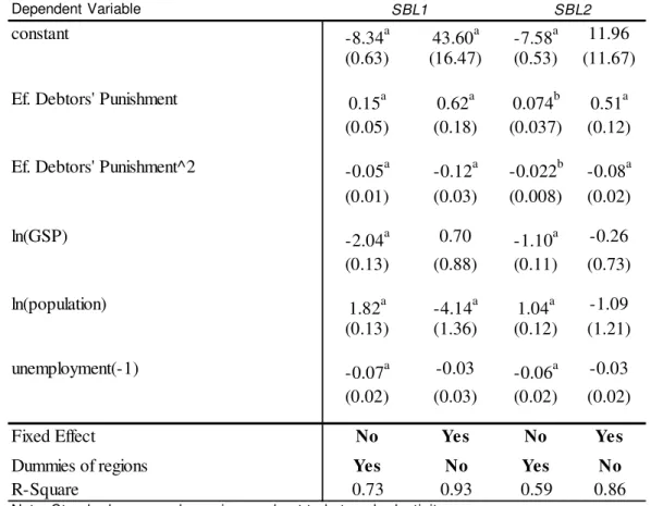
Running the same test for e¤ective debtors’ punishment, table 6 shows that results are again signi…cant in most classes of loans (the exception is SBL3 with …xed e¤ect). For all classes the result of intermediary optimal level of debtors’ punishment still holds, which means that even considering the penalty as a portion of individuals’ income (a real variable instead of a nominal variable) our claim is also valid.

6

Conclusion

The objective of this paper was to study the e¤ect of bankruptcy exemptions on the aggregated level of small businesses and individuals’ loans. We started with a simple model that provides some predictions about the behavior of the demand and supply of credit. On the supply side, the model predicts that as the bankruptcy exemption increases, the interest rates charged to borrowers increase, and when the exemption is su¢ciently high the supply of credit disappears. This is explained by the lower expected repayment and the higher possibilities of strategic default. On the demand side, the model predicts that as the bankruptcy exemption decreases the demand for loans is inhibited due to the fear that borrowers have of losing a signi…cant part of their wealth. To analyze the equilibrium we simulate the model to di¤erent levels of bankruptcy exemptions. The results show that both extreme levels of exemptions (high and low) provide a small level of credit negotiated between the interested parties. As expected, there is an intermediate level of exemption that maximizes the level of credit and welfare in the economy. Therefore, the equilibrium of the volume of credit is a non-monotonic function of the bankruptcy exemption levels, where the optimal level of exemption is intermediary with not too harsh neither too lenient punishment.

After the theoretical approach, we aimed at verifying empirically the e¤ect of bankruptcy exemption on credit. As expected, we …nd a non-monotonic relationship between debtors’ punishment (bankruptcy exemption) and the level of small businesses and individuals’ loans. It means that high bankruptcy exemptions are too lenient with debtors, providing incentive for default which produces a negative e¤ect on the supply of credit, since lenders expect to receive less in these states. On the other hand too low levels of bankruptcy exemptions provide to debtors a harsh punishment in case of default, inhibiting their demand for credit, fearing bad states of nature. Therefore, the optimal bankruptcy exemption is the one that allows a fresh re-start for debtors and a signi…cative recovery for lenders in case of bankruptcy. This level was estimated and the optimal bankruptcy exemption for small businesses and individuals are between ($19;300; $20;146) and ($24;663; $28;645); respectively, with 90% of con…dence: We also notice that just a few states in the U.S. were applying an exemption close to the optimal level, and therefore interventions on the exemption levels would be credit and welfare enhancing.

References

[1] Araújo, A., Monteiro, P. K., Páscoa, M. R., “Incomplete Markets, Continuum of States and Default”, Economic Theory, 11, 205-213, 1998.

vol. 20, no. 3, pp. 455-481, 2002.

[3] Barron, J. M. and Staten, M. E., "Personal Bankruptcy: A Report on Petitioners’ Ability-to-Pay", Credit Research Center, Georgetown University School of Business, mimeographed, 1998.

[4] Berkowitz, J., Hynes, R., "Bankruptcy exemptions and the market for mortgage loans,"

Journal of Law and Economics, 42, 809-830, 1999.

[5] Berkowitz, J., White, M., "Bankruptcy and small …rms’ access to credit", RAND Journal

of Economics 35, pp. 69-84, 2004.

[6] Boyes, W., Faith, R. L., "Some E¤ects of the Bankruptcy Reform Act of 1978," Journal of

Law and Economics, 29, 139-49, 1986.

[7] Djankov, S., McLiesh, C., Shleifer, A., “Private Credit in 129 Countries", working paper, 2006

[8] Domowitz, I., Eovaldi, T., "The Impact of the Bankruptcy Reform Act of 1978 on Consumer Bankruptcy," Journal of Law and Economics, 36, 803-35, 1993.

[9] Dubey, P., Geanakoplos, J., Shubik, M., “Default an E¢ciency in a General Equilibrium Model with Incomplete Markets”, Cowles Foundation Discussion Paper 879R, 1989. [10] Dubey, P., Geanakoplos, J., Shubik, M., “Default and Punishment in a General

Equilib-rium”, Econometrica vol.73, no_{1, 1-38, 2005.}

[11] Dubey, P., J., Shubik, M., “Bankruptcy and optimality in a closed trading mass economy modelled as a noncooperative game”,Journal of Mathematical Economics, 6, 115-134, 1979. [12] Elias, S., Renauer, A., Leonard, R., Michon, K., “How to …le for Chapter 7 Bankruptcy”,

11th edition, Nolo Press, 2004.

[13] Galindo, Arturo, “Creditor Rights and Credit Market: Where do we Stand?”, Seminar: Towards Competitiveness: The Institutional Path, Chile, 2001.

[14] Geanakoplos, J., “Promises Promises”, In W.B. Arthur, S. Durlauf and D. Lane, The

Economy as an Evolving Complex System, II. Reading, MA: Addison-Wesley, pp. 285-320.

[15] Gropp, R., Scholz, J. K., White, M., “Personal Bankruptcy and Credit Supply and De-mand”, 112, Quarterly Journal of Economics, 217-252, 1997.

[16] La Porta, R., Lopez-de-Silanes, F., Shleifer, A., Vishny, Robert W., “Law and Finance”,

Journal of Political Economy 106, pp. 1113-1155, 1998.

[17] La Porta, R., Lopez-de-Silanes, F., Shleifer, A., Vishny, Robert W., “Legal Determinants of External Finance”, Journal of Finance 52, pp. 1131-1150, 1997.

[18] Lin, E. Y., White, M., “Bankruptcy and the Market Mortgage and Home Improvement Loans”, Journal of Urban Economics, 50, pp. 138-162, 2001.

[19] Orzechowski, S. and Sepielli, P., "Net Worth and Asset Ownership of Households: 1998 and 2000", Household Economic Studies, U.S. Cesnus Bureau, 2003.

[20] Peterson, R. L., Aoki, K., "Bankruptcy Filings before and after Implementation of the Bankruptcy Reform Law," Journal of Economics and Business, 36, 95-105, 1984.

[21] Shepard, L., "Personal Failures and the Bankruptcy Reform Actof 1978," Journal of Law

and Economics, 27, 419-37, 1984.

[22] White, Michelle, “Bankruptcy and Consumer Credit in the U.S.”, NBER 2002.

[23] White, Michelle., "Personal Bankruptcy under the 1978 Bankruptcy Code: An Economics Analysis," Indiana Law Journal, 58, 1-53, 1987.

[24] White, Michelle, “Why Don’t More Households File for Bankruptcy”, Journal of Law,

[25] White, Michelle, “"Economic Analysis of Corporate and Personal Bankruptcy Law," NBER working paper 11536, July 2005.

A

Appendix

Proof of Proposition 1. Let

(1 +rf)B = p(C1)(1 +r)B +

X

s

ps[ s d+ (1 s)] [max(w2s+ D E;0) B] be the

function that determines the supply of credit. Let E be equal w2S + D: Thus, for every E

above E the borrowers will …le for bankruptcy in every state of nature since d = 1 for all s;

making pbankruptcy = S

P

s=1

ps = 1: Also, max(w2s + D E;0) = 0; making the supply function

(1 +rf)B = B: The only value of B that satis…es this expression is B = 0:

Proof of Proposition 2. Let

(1 +rf)B =p(C1)(1 +r)B+

X

s

ps[ s d + (1 s)] [max(w2s+ D E;0) B]

Suppose that the bankruptcy exemption E decreases. Thus, w2s+ D E will increase as

well as the probability of solvency since there will be more states of nature that (1 +r)B max(w2s+ D E;0):Both forces work to increase the expected return of lenders. To hold the

equality of the supply function it is necessary to reduce r.

Proof of Proposition 3. To prove it by contradiction let us suppose that ifEincreases toE0_;

B decreases. This condition means that u0

E(c1)< u0E0(c1); because w1+D+B > w1+D+B0:

By the individuals’ maximization problem, ifu0

E(c1)< u0E0(c1)holds, we have S

P

s=h

psu0E(c2s)<

S

P

s=i

psu0E0(c2s); where h and i are the worst states of nature that the agent chooses not …le for

default for E and E0 _{respectively.}

But if B > B0_{, the marginal utility at the second period forE is bigger than for E}0 _that

is u0

E(c2s) > u0E0(c2s) because w2s + D (1 +r)B < w2s+ D (1 +r)B0: Also, since E0

is bigger, the states of nature that the agents …le for default increase (or at least remain the same), thus i hmeaning that the debtors pay their debts in less states (S h S i).

Hence,u0

E(c2s)> u0E0(c2s)andi h) S

P

s=h

psu0E(c2s)> S

P

s=i

psu0E0(c2s), what is a contradiction.

Therefore, if E increasesB increases too.

Moreover, if E ! 1 the marginal cost of the debt is zero (u0

E0(c1) = 0) since min[(1 +

r)B;max(w2s+ D E;0)] = 0:Thus, c1 ! 1 and since w1+D are constant B ! 1:

Therefore, an increase in the bankruptcy exemption makes the demand for credit increase.

Proof of Proposition 4. Let

(1 +rf)B = p(C1)(1 +r)B +

X

s

ps[ s d+ (1 s)] [max(wsB +D E;0) B] be the

function that determines the supply of credit. Let E be equal wSB +D: Thus, for every E

above E the entrepreneurs will …le for bankruptcy in every state of nature since d = 1for all

s; makingpbankruptcy = S

P

s=1

ps = 1:Also,max(wsB +D E;0) = 0;making the supply function