October 30, 2001
Life Expectancy, Educational Attainment, and Fertility Choice
∗Abstract
This paper explores the role of mortality as a determinant of educational attainment and fertility, both during the demographic transition and after its completion. Two main points distinguish our analysis from the previous ones. Together with the investments of parents in the human capital of children, traditional in the fertility literature, we introduce investments of adult individuals (parents) in their own education, which ultimately determines productivity in both the goods and household sectors. Second, we let adult longevity affect the way parents value each individual child. Increases in adult longevity or reductions in child mortality eventually raise the investments in adult education. Together with the higher utility derived from each child, this tilts the quality-quantity trade offtowards less and better educated children, and increases the growth rate of the economy. This setup can explain both the demographic transition and the recent behavior of fertility in “post-transition” countries. Evidence from historical experiences of demographic transition, and from the recent behavior of fertility, education, and growth generally supports the predictions of the model.
Rodrigo Reis Soares
Department of Economics — University of Chicago, 1126 East 59thStreet, Chicago, Illinois, 60637;
∗I owe special thanks to Gary Becker, Steven Levitt, Kevin M. Murphy, and Tomas Philipson for important
1
Introduction
Major demographic changes swept the world in the course of the last century. Today, mortality reductions have reached virtually every corner of the globe — with some unfortunate exceptions — and the vast majority of the world population lives in countries where fertility has already shown a significant decline, and where population is expected to stabilize within the next 50 years (Robinson and Srinivasan, 1997). These are the main features of the so called demographic transition.
Generally, the transition has been characterized by significant reductions in mortality followed by reductions in fertility, implying a period of intense population growth, which progressively diminishes as fertility starts to decline (see Heer and Smith, 1968; Cassen, 1978; Kirk, 1996; Mason, 1997; and Macunovich, 2000). In the demographers’ view, “if there is a single or principal cause of fertility decline, it is reasonable to ascribe it to falls in mortality, which was the major cause of destabilization” (Kirk, 1996, p.379).1
Also, developed countries have recently experienced increasingly low fertility levels. In 1999, countries like Belgium, Germany, and Spain had fertility rates around 1.5, significantly below the replacement rate (' 2.1). Furthermore, several developed countries continue to experience decreasing fertility rates, despite very low fertility levels and the fact that the demographic tran-sition is already completed. This phenomenon has been largely overlooked both empirically and theoretically by the demographic and economic literature. It points to the necessity of under-standing the recent behavior of fertility from a more general perspective, not restricted to the process of demographic transition.
The goal of this paper is to explore the role of life expectancy as a determinant of educational attainment and fertility, both during the demographic transition and after its completion. In the last decades, economists have become increasingly interested in the question of fertility choice and investments in human capital. Although the more recent phenomenon of low and decreasing fertility in developed countries has not received much attention, the process of demographic tran-sition has been the subject of numerous studies (see, for example, Becker, 2000; Becker, Murphy, and Tamura, 1990; Ehrlich and Lui, 1991; Sah, 1991; Meltzer, 1992; Tamura, 1996; Blackburn and Cipriani, 1998; Galor and Weil, 2000; and Kalemli-Ozcan et al, 2000). We believe that our approach improves upon this literature in many respects. We deal with adult longevity, child mortality, human capital, and fertility in a straightforward way, which allows us to understand
1 Initial economic conditions varied a lot in the different experiences of demographic transition. Also, there is
the recent behavior of fertility in the more developed countries, ignored by the above-cited studies and incompatible with most of their results. Additionally, we are able to explain the fertility transition in a more complete fashion.
In the model, mortality is assumed to be exogenous at the individual level, and fertility is assumed to be always an object of individual choice.2 Although there are various actions that agents can take to improve their life prospects, our interest here is focused on the gains in life expectancy observed in the last two centuries, which were largely due to scientific revolutions and technical improvements. At the individual level, these were partly exogenous. And even though these gains were endogenous to the economic system as a whole, they were, to some extent, still exogenous to most of the less developed countries. These countries experienced longevity gains independent of improvements in economic conditions, partly as a consequence of the absorption of knowledge generated elsewhere and of the help provided by international aid programs (see Preston, 1975 and 1980; and Kirk, 1996).
Theoretically, two points distinguish our analysis from the previous ones. First, we let adult longevity affect the way in which parents value each individual child, in much the same way that the number of children does in the traditional literature. This assumption is simply an extension of the widely accepted effect of child mortality on fertility to later ages. Intuitively, it can also be understood in these terms, once one considers that individuals are not only concerned with the survival of their children, but also with the continuing survival of their whole descent. Acknowledging the importance of adult longevity to the way in which parents value each individual child has important consequences in terms of fertility choices. This hypothesis alone helps explain the behavior of fertility after the demographic transition.
Second, together with the traditional emphasis on investments of parents in the human capital of children, we introduce investments of adult individuals (parents) in their own education. This distinction between “basic” and “adult” human capital helps separate the effects of child mortality from those of adult longevity on investments in human capital and growth.3
These two features of our theory play central roles in the mechanics of the model. Briefly,
2The issue of fertility choice in underdeveloped economies is controversial in the demographic literature.
Never-theless, evidence indicates that there is always some margin of choice. Several kinds of actions taken in ‘pre-modern’ societies, directly or indirectly, affect fertility outcomes, including marriage patterns, breast feeding habits, abortion, and sexual practices (see Demeney, 1979; Caldwell, 1981; Kirk, 1996; and Mason, 1997). We abstract completely from this issue here, and assume that fertility was always, at no cost, an object of individual choice. Even though we acknowledge that technical developments made the control over the number and timing of births more precise, we believe that this is an issue more related to the uncertainty of the outcome than to the ideal choice itself, and our interest concerns mainly the latter.
3Furthermore, this approach is more realistic and brings the theory closer to the empirical accounts that justify
increases in adult longevity or reductions in child mortality eventually raise the investments in education, which increase the productivity of individuals both in the labor market and in the household sector. Also, higher life expectancy tilts the quantity-quality trade-offtowards less and better educated children and tends to move the economy out of a “Malthusian” equilibrium. Once the economy abandons the “Malthusian” regime, increases in life expectancy cause reductions in fertility, increases in educational attainment, and increases in the growth rate of the economy.
In the empirical discussion, we present different sets of evidence to support the predictions of the model. We justify the exogenous role played by life expectancy by showing that recent reductions in mortality were largely independent of improvements in economic conditions, so that they indeed appear to be a driving force behind changes in other demographic variables. We discuss historical experiences of demographic transition and argue that, generally, they agree with the patterns generated by the model. Finally, we test the theoretical predictions in relation to fertility, educational attainment, and growth in ‘modern’ economies, using a cross-country panel with data between 1960 and 1990. In brief, the estimated model implies that a 10 year gain in adult longevity reduces fertility by 1.7 points, increases the average schooling in the population by 1 year, and increases the growth rate by 5%; a reduction of 100 per one thousand in child mortality implies a decrease of 1.5 points in the total fertility rate.
The structure of the paper may be outlined as follows. Section 2 motivates the discussion by showing that while the cross-sectional relation between income and some key demographic vari-ables (life expectancy, fertility, and schooling) has been monotonically shifting in the last 35 years, the relation between life expectancy and the same demographic variables has remained consider-ably stable. Section 3 discusses the structure of the model, and the effects of adult longevity and child mortality on both the steady-state with growth and the Malthusian equilibrium. Section 4 summarizes the theoretical results and describes histories of demographic transition that would be expected to arise from our model. Section 5 discusses how the model fits the empirical evi-dence. We discuss how some recorded demographic transition histories fit the patterns described in section 4, and analyze whether the more recent cross-country behavior of fertility, education, and growth supports the predictions of the model. Thefinal section summarizes the main results of the paper.
2
The Behavior of Life Expectancy, Fertility, and
Educa-tional Attainment after the Demographic Transition
income improve nutrition and health consumption, which reduces mortality rates; income gains also change the quantity-quality trade off in terms of number and education of children, which reduces fertility and increases human capital investment. Statements like these are common places in the economics profession, and it seems fair to say that they give an accurate description of the consensus regarding the main changes taking place during the process of economic development.
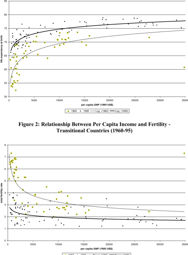
Even though there is obviously a lot of truth to this view, it is far from giving a complete picture of reality. Recently, the relationship between income and crucial demographic variables, such as life expectancy or fertility, has been clearly unstable. Figures 1 to 3 illustrate the changing relationships between income, life expectancy, fertility, and educational attainment.4 To concen-trate on economies that share the same demographic regime, the figures refer only to countries that had already started the demographic transition in 1960.5
Figure 1 shows that, for constant levels of income, life expectancy has been rising.6 Logarithm curves are fitted to the 1960 and 1995 cross sectional relation between per capita GNP and life expectancy. For lower levels of income, life expectancy at birth has increased by more than five years in the period between 1960 and 1995. This means, for example, that a country with per capita GNP of US$5,000 in 1995 had a life expectancy roughly 10% higher than a country with per capita GNP of US$5,000 in 1960.
Figure 2 tells an analogous story for the relationship between income and fertility. Again, curves are fitted to the 1960 and 1995 cross sectional relationship between income and fertility. For constant levels of income, fertility has been falling. These reductions have been as large as 2 points for countries with per capita income around US$3,000, and even larger for poorer countries. Finally, as Figure 3 shows, the story is not different for the relationship between education and income. Logarithm curves are fitted to the cross sectional relationship between income and average schooling in 1960 and 1990. Gains in average schooling in the period were usually over 1 year, for constant levels of income.
One immediately wonders whether these changes in life expectancy, education, and fertility are interrelated, and what the specific mechanisms connecting them are. An insight in this direction
4 The general results illustrated in Figures 1 to 5 do not depend in any way on the specific statistics used, or
on the presence of any particular country in the sample. Detailed description of the variables is saved until the empirical section. The logarithm curves used are of the general formy=α+βln(x),and the power curves used are of the general formy=αxβ.
5A more precise reason for the restricted sample is given in the theoretical section. Empirically, some objective
criterion defining whether a country already started the demographic transition has inevitably to be chosen. Our choice is the cutoffpoint ”countries that had life expectancy at birth above 50 years in 1960”, also to be justified later on. The results do not depend on the specific criterion chosen, and we believe that there should not be much discussion regarding the countries actually included in the sample (generally, OECD, Latin American, East Asian, and some Arab and North African countries).
is gained by looking at the relation between life expectancy and the other two variables.
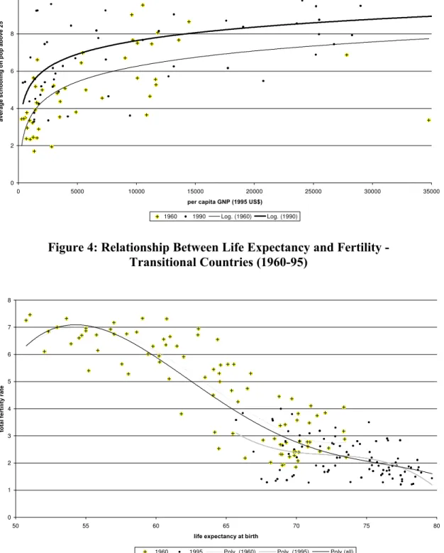
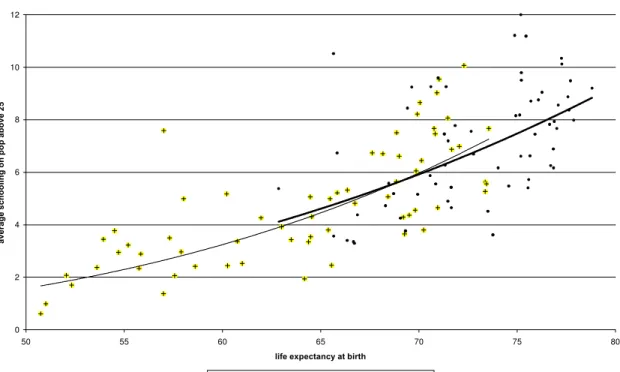
In Figure 4, we plot the cross sectional relation between life expectancy and fertility in 1960 and 1995. The lines are polynomials (3rd order)fitted to the different years.7 Atfirst sight, the shift in the position of the curve suggests that a change in the relationship is being portrayed. But if we look closely, there is not much overlapping of the two curves, and when the overlapping does actually occur, the points relative to the different years are more or less evenly distributed over the same area. The two segments look more like an approximation to a single stable nonlinear function than a description of a changing relationship. This point is further explored by fitting a single nonlinear function (3rd order polynomial) to the whole data set, assuming that a stable relation
is present throughout the period. Visually, the curve seems to have a goodfit, and the functions estimated separately for each sub-period seem to merge into it. The single fitted line actually explains more of the overall variation in the data than the two polynomials fitted independently to each year (R2of 0.78, against 0.76 for 1960 and 0.21 for 1995). The interesting part is that this curve does not separate points from 1960 and 1995 as being below or above it, as a curve fitted to all the data in Figures 1, 2, or 3 would do. Points from the different years are distinguished as being more on its left portion or on its right portion, as if countries were sliding on this curve through time, via increases in life expectancy and reductions in fertility.
The results regarding life expectancy and educational attainment are even stronger. Figure 5 plots the cross sectional relationship between these two variables in 1960 and 1990, and fits a power curve to each year. The stability of the relationship through time is clear. Indeed, the two curves almost merge into each other for the region over which there are observations for both years. Again, countries seem to be sliding on this curve through time, as life expectancy and educational attainment rise simultaneously.
So, for constant income levels, life expectancy is rising, fertility is declining, and educational attainment is increasing. At the same time, changes in fertility and schooling are following very closely the changes in life expectancy, such that, for constant life expectancy at birth, these variables seem to be constant. While fertility and education are direct objects of individual choice, life expectancy has a large exogenous component, related to scientific knowledge and technological development. This reasoning suggests that exogenous reductions in mortality together with a stable behavioral relationship between life expectancy and the other demographic variables are the driving forces behind these changes. In what follows, we develop a theory along these lines. Our goal is to explain the facts discussed above, together with the triggering of the demographic transition, as being determined by exogenous increases in life expectancy.
3
Theory
3.1
The Structure of the Model
Assume an economy inhabited by adult individuals, who live for a deterministic amount of time, when they work, consume, invest in their own education, have children, and invest in the education of each child. The model is the usual ‘one sex model,’ common to the fertility literature. We abstract from uncertainty considerations, to concentrate on the impact of adult longevity and child mortality on the direct economic incentives at the individual level. To make the model treatable, we also abstract from the presence of physical capital. Individuals, or households, have an endowed level of what we call ‘basic’ human capital (determined from previous generation’s decisions), based on which they decide on how much to invest in their own ‘adult’ education. Adult education determines productivity both in the labor market and in the household sector. Households possess backyard technologies for producing goods, adult human capital, and basic human capital, and they decide on how to allocate their time across these different activities in order to maximize utility. As we will see later on, changes in adult life expectancy and child mortality will change the incentives to engage in these different activities.
In the model, adults live forT periods, and at ageτ they have children. A fractionβ of the born children dies before reaching adulthood. Parents derive utility from their own consumption in each period of life (c(σt)σ), and from the children they have. Childhood can be thought of as an instantaneous phase: as soon as individuals are born they become adults, and there is no decision to be taken as a child.
We assume that adults are concerned directly with the level of human capital of their children, via a constant elasticity function hαc
of each individual child. Therefore, (1−β)nT assumes the role usually played bynalone in the traditional economic analysis of fertility. Intuitively, this set up extends the logic usually applied to the child mortality rate to later ages. It is a natural extension, once one considers that individuals are not only concerned with the survival of their children, but also with the continuing survival of their whole descent.8 Additionally, we also assume that there is a tendency towards satiation in terms of the total of child-years, in the sense that for sufficiently high values, its marginal utility is zero. This seems to be a sensible hypothesis once, holding T constant, we think about the biological constraints that nature imposes on the bearing and timing of births. It will also be important to assure that increases in life expectancy will eventually move the economy out of a Malthusian equilibrium.
Individuals face goods and time constraints: they have to allocate their total lifetime between working (l), raising kids (b), and investing in their own education (e); and they have to allocate goods between their own consumption and children’sfixed costs (f). Parents’ income is determined by how much human capital they have (Hp) and by how much they work, and borrowing from
future generations or monetary bequests are not allowed. Finally, we assume that the production functions of adult human capital, basic human capital, and goods are multiplicative on human capital and time. This means that adult human capital increases the individual’s productivity both in the labor market and in the household production of basic human capital, and that basic human capital increases the productivity of education in generating adult human capital.
Given these assumptions, individuals solve the following problem (IP):9
max
{c(t),n,l,b,e}t∈[0,T]
T
Z
0
exp(−θt)c(t) σ
σ dt+ρ[(1−β)nT]
hα
c
α
(IP)
subject to
8In this case, individuals take into account that their children will need enough time to have their own children
and raise them.
9Additionally, if we assume that parents enjoy having children only to the extent that they share part of their
lifetime, the second term in the expression has to be integrated over time fromτtoT, and discounted at the rate
y >
T
Z
0
exp(−rt)c(t)dt+ exp(−rτ)nf, T > l+bn+e,
Hp = Aehp+Ho,
hc = DbHp+ho,
y = lHp,
hp given.
where D, A >0; 0<σ,α<1;u0(.),ρ0(.)>0;u00(.),ρ00(.)<0;ρ0(x) = 0 for somex=x >0. f is the goodsfixed cost of having a child,bis the time investment in human capital per child, and eis the time devoted to adult education. c(t) is adult consumption at instant t,l is lifetime labor supply, nis the number of children, and ρ(.) is an increasing and concave function. D, A,
Ho, and ho are technological parameters, r is the interest rate, andθ is the subjective discount
rate.
We distinguish between basic human capital and adult human capital: hdenotes the kind of human capital formed during childhood, in which parents can invest, related to basic education and skills, and emotional development;H denotes the kind of human capital that can be obtained during young adulthood, related, for example, to college or graduate education, or to professional training. This set up assumes that individuals enter adulthood with a given level of basic education (hp), and then, by deciding on how much to invest in their own education, they choose a level
of adult human capital (Hp). hc is the level of basic human capital that parents gives to each
of their children. Ho and ho denote the levels of adult and basic human capital that individuals
have, even in the absence of investments of any sort in education, maybe determined from innate skills or natural learning throughout life. As will be clear in the following sections, these factors play an important role in allowing for the existence of a so called Malthusian steady-state, with no investment in human capital and zero growth.
To concentrate on the issues of interest, we depart from this formulation and introduce some simplifying assumptions. Since our central interest is the long run behavior of the economy, mainly the inter-generational fertility and human capital decisions, we abstract from life cycle considerations by assuming that subjective discount rates and interest rates equal zero. Given the separability of the utility function over time, this implies constant consumption throughout life.
max
{c,n,l,b,e}
½
Tc
σ
σ +ρ[(1−β)nT]
hαc
α ¾
,
and
lHp>T c+f n.
This is the benchmark model that guides our theoretical discussion. In the next subsection, we analyze the effects of adult longevity on educational attainment, fertility, and economic growth.
3.2
The Role of Adult Longevity
3.2.1 Static Implications of Longevity Gains
In this subsection, we look at the individual decision taking the initial level of basic human capital as given (hp). In the following subsections, we discuss the implications of this decision process to
the growth rate and dynamic behavior of the economy, and look at the properties of an equilibrium with zero growth and no investments in human capital.
As we hold child mortality constant, we save in notation by omitting the parameterβ. Also, given that we look at an equilibrium with growth, the parametersf,ho, andHobecome irrelevant
as time goes by, so we ignore them. Defining Ap =Ahp, Dp =DAp =DAhp, substituting for l in the time constraint, and for hc in the utility function, the first order conditions (foc’s) for,
respectively, c,n,b, andecan be written as:
T cσ−1 = T
Ape
λ, (1)
Tρ0(nT)(Dpbe)
α
α = bλ, (2)
ρ(nT)(Dpbe)α−1Dpe = nλ, (3)
ρ(nT)(Dpbe)α−1Dpb =
µ
1− T c
Ape2
λ; (4)
where λis the multiplier on the constraint above. Using equations 2 and 3 from the foc’s, we get:
nTρ 0(nT)
ρ(nT) =α. (5)
Ifε(.) is monotonic, this implies thatnT will always be constant, and that exogenous changes in T will have the following effect onn:
dn
dT =−
ε0(nT)n
ε0(nT)T =− n
T <0. (6)
The equalization of elasticities expressed in equation 5 comes from the fact thatnandbenter in a multiplicative way both in the objective function (via the sub-utility functions) and in the constraint. But the simple expression obtained above hinges on the additional assumption of constant elasticity for the hc sub-utility function. What this buys us is the independency of n
in relation to all other exogenous variables apart from T. With a more general specification,
hc would show up in the right hand side of 5, and it would allow the other exogenous variables
to affect the optimal choice of n. But also in this case, the force working towards a negative relationship between nand T would still be present, even though it could possibly be weakened by the adjustment onhc. The important factor here is the presence ofT in the discount function
ρ(.), and the way in whichT andnenter inside this function. As long as we have a specification wherenandT have similar effects onε(.), there will be a tendency fornandT to move in opposite directions.10 This is the role played here by the assumption that parents see number of children and adult lifetime of each child in similar ways, such that the relevant variable in determining how much parents care for each individual child is the total lifetime of the children, or the total of ‘child-years’.
Using equations 1, 3, and 4 from the foc’s, we get:
Ape2 = T c+Apebn, (7)
ρ(nT)(Dpbe)α−1D = ncσ−1. (8)
The constraint gives usT c+Apebn=T Ape−Ape2. Together with equation 7, this implies
e=T
2, and
de
dT =
1
2. (9)
Educational attainment increases with longevity. This should be expected, since increases in longevity increase the period over which the returns from investments in education can be
10More precisely, if the altruism function assumes the general formρ(n, T), andε(n, T) =ρn(n,T)n
ρ(n,T) denotes its
elasticity in relation ton, the condition for dn
dT to be negative is thatsign{εn(n, T)}=sign{εT(n, T)}, where the
enjoyed. Technological parameters, such asAandD, do not appear in expression 9 because they affect the costs and benefits of investments in education in the same way.11 Although we see
e here as a measure of educational attainment, it can also be regarded in more general terms as the specialization of individuals in the social division of labor. In this sense, this result is the one observed by Becker (1985) and Becker and Murphy (1992), where increases in the total time available for labor market activities tend to increase the amount of specialization.
With expressions 6 and 9 in hand, we can use equations 7 and 8 to determine the effects of exogenous changes inT oncandb (see Appendix A.1). This gives us
db
dT =
−nncσ−1h1
T + (1−σ) Ap
2c( bn
T +
1 2)
i
+ρ(nT)(α−1)(Dpbe)α−2DDpb2
o
ρ(nT)(α−1)(Dpbe)α−2DDpT2 −(1−σ)n2cσ−2A2p
≶0,
and
dc
dT =
Ap
n
n2cσ−1hT1 + (1−σ)Ap 2c(
bn T +12)
i
+ρ(nT)(α−1)(Dpbe)α−2DDp(nb+T4)
o
ρ(nT)(α−1)(Dpbe)α−2DDpT−(1−σ)n2cσ−2Ap ≶
0.
Both dc dT and
db
dT can be either positive or negative, but, as shown in Appendix A.1, they cannot
be both negative at the same time. cor bmust necessarily increase asT increases, and both can increase at the same time. This is an obvious result once we realize that an increase in T also means an expansion in the constraint set. Sincengoes down asT increases, andeincreases only proportionally toT, the additional resources have to be ‘consumed’ either via a raise inb or via a raise inc, and possibly via both.
The specific signs of dc dT and
db
dT depend on the values of the parameters, but the forces at
work can be understood by looking at the individual problem. We know that, asT increases, the shadow price of the timeb invested inhc (n) goes down, and the productivity of this investment
goes up (e), so that hc must increase in the new optimum, even though b itself may decrease.
Depending on the magnitude of the decrease in this shadow price, and on the concavity of the sub-utility functions (σandα), it will be worthwhile for the individual also to increasectogether withhc, or to letcdecrease ashc increases.
It is easy to show that hc unequivocally increases as T increases. Since hc =Dpbe, we have
that dhc
dT =Dp(b de dT +e
db
dT), which gives: dhc
dT =
−Dp
©
2cσ−1n£1 + (1−σ)bn c Ap
¤
+ (1−σ)ncσ−2A
pT2
ª
ρ(nT)(α−1)(Dpbe)α−2DDpT+ (σ−1)n2cσ−2Ap >0.
11This result is analogous to the one originally obtained by Ben-Porath (1967), regarding the effect of the price
It may seem counterintuitive thatcmay actually go down asT increases, but it is important to keep in mind exactly what this theoretical experiment corresponds to. Here, we are analyzing an increase inTholding constant the level of basic human capital of parents (hp). So, the result means
that individuals entering adulthood that face an increase in their life expectancy will increase their own education and the basic education that they give to their children. And it may even be the case that they reduce their own consumption in each period in order to be able to invest more in the children’s human capital. This is different from analyzing what will be the effect of T on the consumption pattern across generations. As we will see now, the model predicts that increases in
T increase the growth rate of consumption across generations.
3.2.2 Dynamic Implications of Longevity Gains
The Possibility of a Steady-State
The possibility of a steady-state in this economy rests on the values of the parameters αand σ. Technological factors summarized by the goods constraint in problem IP imply that, in any
steady-state,candhp must necessarily grow at the same constant rate from one generation to the
next. But the individual maximization problem tells us, through equation 8, thatcandhpgrowing
at the same rate will not be consistent with the optimal choices of the different generations, unless α=σ. Therefore, for a steady-state to exist in this economy, it must be the case thatα=σ, so that individuals from different generations will make optimal choices such thatcandhpwill grow
at the same constant rate, andb,n,e, andl will be constant.
This can be formally seen once we realize that, in terms of the individual problem stated in IP, for a steady-state to exist it must be the case that the agent will not change his decisions regardingn,b,l, andeashpincreases. This means that the different generations, who differ only
in terms of their endowed hp and see it as a given parameter, will translate the higher levels of
basic human capital in increased consumption, leavingb,n,e, andl unchanged.
From the results obtained before, we already know that dhdnp =dhdep = 0. We can use equations 7 and 8 to show how bandcrespond to changes inhp. This gives the following expressions:
db dhp
= (σ−1)be
hp[(σ−α)bn+ (α−1)e]− b hp ≷
0, and
dc dhp
= Ae
2(1−α)(bn−e)
T[(σ−α)bn+ (α−1)e] >0, where the sign of dc
dhp comes from the fact thatσ<1.
As mentioned before, a steady-state requires a constantbwith an increasinghp. This will only
happen here ifσ=α, in which case we have db
dhp = 0 and
dc dhp =
A
that, in this case,candhp will grow at the same constant rate, given by (1 +γ) = hhcp =DAbe. Ifσ6=α, there is no steady-state, andbwill increase or decrease over time (with the increase in hp) until a corner solution is reached. Rewrite dhdbp in the following way:
db dhp
= b
hp
(σ−α)(e−bn) [(σ−α)bn+ (α−1)e]. So, ifα>σ, we have db
dhp >0; and if α<σ, we have
db
dhp <0, sinceσ<1.
The intuition for this result is clear. If α >σ, the sub-utility function related to hc is less
concave than the one related to c, such that when hp grows from one generation to the next,
younger generations tend to increase hc more than proportionately to c, and this is achieved
through increases inb. The same sort of argument works for the case whereα<σ, implying that
hc is increased less than proportionately toc, and that this is achieved through reductions inb.
Whenα=σ, every generation is just happy to increasecandhpin the same proportion in relation
to the previous generation, in which casebremains unchanged and we have a steady-state. If this actually happens, we will necessarily have hp and c growing at the same constant rate through
time. From now on, when discussing an equilibrium with growth, we will implicitly assume that α=σ, so that a steady-state exists.
The Effect ofT on the Steady-State Growth Rate
The production function ofhc implies that the growth rate of basic human capital is given by12
(1 +γ) = hc
hp = DAbe. From the goods constraint on problem IP we have that Ahple = T c, which implies that, in steady-state,cwill grow at the same rate ofhp, namely, (1 +γ). The same
will also be true for the level of adult human capital (Hp), as can be seen from the production
functionHp=Aehp.
The effect of longevity gains on the growth rate of this economy is given by
d(1 +γ)
dT =DA
µ
bde
dT +e
db dT
>0, where the sign comes from the fact that, as proved in subsection 3.2.1,¡bde
dT +e db dT
¢
>0. Longevity gains increase the steady-state growth rates of consumption and all forms of human capital across generations.
We see the intuition for these results as follows. As longevity increases, incentives to invest in adult human capital increase, so thate— the amount of time devoted to parent’s own education,
12IfDAbe <1, there is no growth in steady-state. In this case,H
oandhowill be important in determining the
or the educational attainment — increases. Once educational attainment and adult human capital (Hp) are higher, the individual becomes more productive in investing in children’s human capital.
The higher life span of each child also tilts the quantity-quality trade offtowards less and better educated children, what reduces fertility. Together with the higher adult productivity in the household sector, this increases the level of basic human capital given to each child. Higher basic human capital, and more investments in adult education (higher educational attainment), end up increasing the growth rate of the economy.
The goal of this section is to stress the role played by adult longevity, through changes in the return to education and the way parents value each child, in the fertility and educational choices. Even though the unambiguity of some of the effects depends on the functional forms adopted, these forces will always be at work, no matter how the model is specified. Our approach shows that, under reasonable assumptions, the role played by longevity gains is important enough to reduce fertility, increase educational attainment, and raise the growth rate of the economy.
3.2.3 The Malthusian Equilibrium
The model developed in the previous subsections can, with little modifications, accommodate a so called Malthusian equilibrium, where investment in all forms of human capital are at corner solutions and fertility varies positively with consumption and production. Besides, the model allows the characterization of the fertility transition as a natural consequence of the escape from such a steady-state, caused by successive increases in adult longevity.
We reincorporate the goodsfixed cost of children (f) and the lower bound levels of basic and adult human capital (ho and Ho) into the model. As mentioned before, in an equilibrium with
consumption and all forms of human capital growing, these constant terms become irrelevant, and all conclusions discussed in the previous subsections hold. But in an equilibrium with zero growth and no investment in human capital these elements play a key role.
A Malthusian equilibrium in this set up is a situation wherehp=ho, and the optimal choice
of the individual implies b=e= 0. Collapsing all the constraints into only one and writing the problem in terms of{c, n, b, e}, this equilibrium is characterized by the following foc’s, whereλis still the multiplier on the constraint:
cσ−1 = λ
Ho ,
Tρ0(nT)ho
α
α =
f Ho
λ,
ρ(nT)hαo−1DHo < nλ,
0 <
·
1−Aho(T cH2+f n)
o
We call this corner solution a Malthusian equilibrium because, in a situation like this, changes in productivity — brought about, for example, by exogenous changes in Ho — will be positively
correlated with changes in both consumption and fertility (for proof and further discussion, see Appendix A.2).
While this corner solution holds, changes inT will only be associated with changes in cand
n. Working with thefirst two foc’s and the constraint, we get the effects ofT oncandn:
dn
dT =
f2n
T2 (σ−1)cσ−2− hαo
α[nTρ00(nT) +ρ0(nT)]
T2ρ00(nT)hαo α +
f2
T(σ−1)cσ−2
≶0, and
dc
dT =
fh
α
o
α[2nTρ00(nT) +ρ0(nT)]
T3ρ00(nT)hαo
α +f2(σ−1)cσ−2
≷0.
Appendix A.2 shows that dc dT and
dn
dT may be positive or negative, but both cannot be negative at
the same time. Either cor nmust increase asT increases, since an increase inT corresponds to an outward shift in the constraint. Besides, −nTρ00(nT)<ρ0(nT)<−2nTρ00(nT) is a sufficient
condition for both dc dT and
dn
dT to be positive. The specific signs of dc dT and
dn
dT depend on the
properties of the ρ(.) function. This is expected, since the only way by which T changes the equality between marginal rate of substitution and price ratios of n and c is via the marginal utility ofn(see foc’s above).
While stuck in this Malthusian equilibrium, an economy can behave in many distinct ways as longevity increases: cand nmay increase, cmay increase and n decrease, or nmay increase and cdecrease. But as T keeps growing, no matter what happens to n and c, the inequalities characterizing the Malthusian equilibrium (last two foc’s above) are eventually broken, and the economy enters in the dynamic process described in the previous subsections, where consumption and human capital grow from one generation to the next, and fertility declines with increases in longevity. Appendix A.2 proves this claim.
sufficiently high, fertility will stop increasing and investments in children’s human capital will be eventually undertaken (makingb >0). If this assumption holds, sufficiently large adult longevity can always guarantee positive investments in adult and basic human capital (b ande >0). After this threshold point is reached, further increases in longevity trigger the demographic transition, and the economy moves into a sustained growth path.
In this setup, the only engine behind the demographic transition and the escape from the Malthusian steady-state is the exogenous change in longevity. In the next subsection, we show that reductions in child mortality can play a similar role, both in terms of the steady-state with growth and the escape from the Malthusian equilibrium.
3.3
The Role of Child Mortality
3.3.1 Child Mortality in the Equilibrium with Growth
We now reintroduce child mortality into the analysis, under the assumption that costs related to having and educating children depend on the total number of born children. Under this assump-tion, the individual problem is exactly the same stated in the beginning of section 3. We start by analyzing the static implications of child mortality reductions, and then go on to discuss its effects on the growth rate of the economy and on the possibility of escape from the Malthusian steady-state. First order conditions for the equilibrium with growth are identical to the ones from section 3.2.1, apart from equation 2, which becomes
(1−β)Tρ0[(1−β)nT](Dpbe)
α
α =bλ, (2’)
and from the fact that (1−β) should be introduced multiplying nT inside ρ(.), wheneverρ(.) appears.
To explore the properties of this equilibrium as β changes, we follow the same steps from subsection 3.2.1. Using equations 2’ and 3, we get
ε[(1−β)nT] =α,
so that dn dβ =
n
1−β >0. The model implies a constant total lifetime of surviving children. In a sense, parents have a kind of target of ‘child-years’, and they increase fertility when child mortality increases, to guarantee the achievement of this ‘goal.’
db
dβ =
(σ−1)bncσ−2−2cσ−1 Ap
(1−β)[(1−σ)ncσ−2+ρ[(1−β)nT](1−α)hαc−2D2T
n ]
<0, and
dc
dβ =
ρ[(1−β)nT](α−1)hα−2
c DpDeb+ncσ−1
(1−β)[(1−σ)ncσ−2+ρ[(1−β)nT](1−α)hαc−2D2T
n ]
≶0.
Also, since hc =DAehpb, we have dhdβc <0.
In an equilibrium with growth, reductions in child mortality will reduce fertility, increase investments in basic human capital, and leave adult educational attainment unchanged (so that
hc will increase). Parents’ consumption may go either up or down, depending on the value of the
parameters.
The growth rate of this economy is given by (1+γ) =DAeb, so it is easy to see that when there is a change inβ, this rate changes by d(1+γ)dβ =DAedb
dβ <0.Increases in child mortality reduce the steady-state growth rate of the economy, via reductions in the investment in basic human capital. Here, the main engine is the reduction in fertility. As child mortality decreases and fertility is reduced, resources are freed up to be used either in producingcor hc. But the reduction in n
also represents a reduction in the shadow price ofhc in relation toc, such thathc will certainly
increase (via an increase in b), and c may go either up or down, depending on how strong the income effect is.
3.3.2 Child Mortality and the Malthusian Equilibrium
We use the same strategy adopted in subsection 3.2.3 to characterize the Malthusian equilibrium in this economy. In this case, the corner solution yields:
ε[(1−β)nT] > αDf ho
, and
T Aho < Ho,
which are analogous to the inequalities obtained before. The behavior ofnandcin this equilibrium can be analyzed using the foc’s and the constraint:
dn
dβ =
Th
α
o
α{ρ0[(1−β)nT] + (1−β)nTρ00[(1−β)nT]} (1−β)2T2ρ00(nT)hαo
α +
f2
T(σ−1)cσ−2
≶0, and
dc
dβ =
−fh
α
o
α{ρ0[(1−β)nT] + (1−β)nTρ00[(1−β)nT]} (1−β)2T2ρ00(nT)hαo
α +
f2
T(σ−1)cσ−2
Note that these two expressions will never have the same sign: if one is positive, the other must be negative. This had to be the case, since changes inβdo not change the individual constraint, so that if the agent wants to increase the ‘consumption’ of some ‘good’, he has to decrease the ‘consumption’ of the other.
Anyhow, no matter what happens to n and c, reductions in child mortality will increase the total number of surviving ‘child-years’ ((1−β)nT), and will push the economy away from the Malthusian steady-state, into a steady-state with growth and positive investments in human capital. The difference here is that, at first, whenβchanges, nothing happens to the incentives to invest in adult human capital (second inequality), and only investments in basic human capital are undertaken. Only after basic human capital (hc) is accumulated from one generation to the
next, the incentives to invest in adult education increase. And if child mortality reduction is large enough, the economy enters a sustained growth path. These claims are proved in Appendix A.3.13
3.3.3 Costs of Children Depending on Number of Surviving Children
In our analysis of the effects of child mortality, we assumed that costs of children depend on the number of born children. Our results would change sensibly if costs of having children depended on the number of surviving children. Which one of the two specifications is the most accurate description of reality is an empirical matter. It probably depends crucially on which phase of childhood concentrates most of the reductions in mortality. We come back to this discussion in the empirical section, but now we briefly explore the theoretical consequences of changing the assumptions related to the costs of having children.
Once we assume that costs of children depend on the number of surviving children, the time and goods constraint in problem IP have to be substituted by the following:
lHp > T c+f(1−β)n, and T > l+b(1−β)n+e,
and the rest of the problem remains unchanged.
The only role of a change in child mortality in this set up will be to change the fertility rate, in such a way as to maintain exactly the same number of surviving children (n, the net fertility
13There are some appealing variations of the basic model that do not introduce any major change in terms of
rate), given constant values of the other parameters. Since child mortality affects the costs and benefits of having children in the same way, parents have a target number of surviving children that is kept no matter what is the child mortality rate. Reductions in child mortality reduce the fertility rate, and leave the other variables unchanged. There is no effect on growth or human capital accumulation, and reductions in child mortality do not tend to move the economy out of a Malthusian regime.
4
Synthesis of the Predictions of the Model
This section takes a step back and looks at the predictions of the model from a broader perspective. We describe histories of demographic transition that would come out of a model as the one outlined in the previous section. We look descriptively at the possible paths that an economy starting from a Malthusian equilibrium would follow as improvements in adult longevity and child mortality took place. Predictions related to adult longevity are basically the same across all the different specifications discussed. In relation to child mortality, predictions may be quite different, depending on the assumptions related to the costs of raising children.
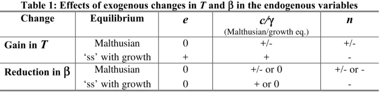
We concentrate the discussion on fertility (n), educational attainment (e), and consumption or growth (corγ), as exogenous changes are assumed to take place in child mortality (β) and adult longevity (T). Table 1 summarizes the effects ofT andβon these three endogenous variables.
For economies starting from the Malthusian equilibrium, the effects of T and β are very similar. At first, educational attainment does not change, while consumption and fertility may go either up or down. In any case, we know that increases in T and reductions inβ will tend to move the economy out of the Malthusian equilibrium, and into a steady-state with growth and investments in human capital. Given our assumptions, in the moments preceding the threshold of this transition, individuals will generally be in a situation where ε[(1−β)nT] has relatively small values, due to an almost constant ρ[(1−β)nT], and a decreasing ρ0[(1−β)nT] (equal to
zero for big enough (1−β)nT). This implies that the terms onρ0(.) andρ00(.) in dn dT and
dn dβ will become quantitatively less important, the closer we are to the beginning of the transition. If this process is strong enough such thatρ0(.) andρ00(.) become irrelevant in determining the signs of dn dT
and dn
but will not change with reductions in child mortality. In our set up, there is nothing that ties down the equilibrium fertility to some specific value. As long as life expectancy keeps growing, fertility will be reduced, possibly to values below replacement rate.
Another variable that deserves special attention from the perspective of the demographic tran-sition, but that we did not mention yet, is population. At any point in time, population is an intricate function of the cumulative effect of past fertility and child mortality rates on initial pop-ulation levels, and also a function of adult longevity. If we normalize our model in such a way that parents have children in the end of theirfirst period of life (τ= 1), and we callPsthe population
at periods, we have that:
Ps= s−1 X
j=s−T
" j Y
i=s−T
(1−βi)ni
#
Ps−T−1=
s−1 X
j=s−T
" j Y
i=0
(1−βi)ni
#
P0,
where s > T, and P0 is the initial population.
This expression helps understand the direct effect of longevity on population size. For illustra-tional purposes, assume an economy in a Malthusian long run equilibrium, where the net fertility rate (n = (1−β)n) equals one. If this has been the case for a sufficiently long time, we have that Ps =Ps−T−1
TP−1
j=1
[(1−β)n]j =P
s−T−1(T −1). Additionally, assume that the fertility rate
does not respond much to changes in adult longevity in this equilibrium, such that dn
dT '0. In
this case, gains on T are translated in an almost one to one basis into population increases: for
T large enough, a 50% gain in adult longevity will represent a long run increase of almost 50% in population.
With child mortality reductions, the effects are even more dramatic, given the cumulative way in which it enters the determination of population size. Even if fertility falls, as long as its fall does not offset completely the child mortality reduction, the long run effects will be enormous. This is clear once we look at the net fertility rate n as a single variable. If we start from a Malthusian equilibrium wheren= 1, and there is a reduction in child mortality that is not completely offset by fertility declines, we will end up in a situation wheren >1. Given constant values for the other parameters,n determines alone the rate of population growth and, thus, anyn >1 represents a population growing exponentially at a constant rate through time. No matter how low this rate is, this means population explosion in the long run.14
What this means is that, as adult longevity increases and child mortality declines, and as the economy approaches the transition point, population should be growing considerably fast. This is even more so once we remember the point mentioned earlier, that, on the verge of the transition,
fertility is likely to rise with adult longevity and not to be very responsive to child mortality changes. And, from a simple accounting perspective, the growth will be faster, the faster are the longevity gains and child mortality reductions.
Thus, our model predicts that Malthusian economies experiencing increases in life expectancy ((1−β)T) would go through an initial phase with consumption and fertility changing in different ways, and with population increasing rapidly. This population increase would be driven mainly by the gains in life expectancy itself. If these gains were significant enough, economies would move to a new equilibrium with growth. From this point on, educational attainment would start rising and fertility would be reduced as life expectancy raised. Further increases in life expectancy in this new equilibrium would be associated with further reductions in fertility, and increases in growth and educational attainment. These are the basic facts that we will be looking for in our empirical investigation of the demographic transition, and of the recent behavior of fertility, educational attainment, and growth in post-transition countries.
5
Empirical Evidence
5.1
The Nature and Timing of Mortality Changes
The engine behind the demographic transition in the theory discussed above is the exogenous rise in life expectancy. For the model to be empirically relevant, it must be the case that longevity gains actually preceded fertility reductions in the real experiences of demographic transition, and that the mortality reductions were to some extent exogenous to economic development. Economic growth, maybe determined by technical development, could be the driving force behind the whole process, reducing mortality via improved nutrition and living conditions, and reducing fertility via the usual income induced quantity-quality trade off. To show that mortality was, per se, a driving force in the process, we have to show that some of the changes in life expectancy were not due to material improvements, nor to changes in behavior induced by increased income.
We do not claim that improvements in living conditions do not affect life prospects. This rela-tion is, indeed, an important part of the mechanism of checks and balances behind the Malthusian model. Our claim is just that changes in life expectancy at birth from 40 to more than 70 years, like the ones experienced during the demographic transition, are not entirely due to material improvements.
accounted for by improved nutrition, so that a gain of 10% in the probability of survival seems to come from sources unrelated to improved material conditions. It is also interesting to note that exactly from 1870 on, the French crude birth rate started to show a consistent declining trend.
The evidence for the less developed countries also indicates that a considerable part of the gains in life expectancy was not related to economic development. Preston (1980) discusses in detail the causes of mortality declines in less developed countries during the twentieth century, and argues that approximately 50% of the decline was not directly related to improved material conditions.
The evidence comes both from the changing relation between economic development and life expectancy, and from the diseases responsible for mortality declines. The changing cross-sectional relation between income and life expectancy was already mentioned (see Figure 1). Similar evi-dence is available regarding the relation between life expectancy and nutrition. Table 2, reproduced from Preston (1980, p.305), contains information on life expectancy at birth in 1940 and 1970, for countries at different income and nutrition levels. Life expectancy gains took place in all the nutrition brackets shown in the Table. For the lowest nutrition group (less than 2,100 calories daily), there was an increase of 10 years in life expectancy at birth. Preston (1980) also relates life expectancy changes to income and calories consumption, and concludes that approximately 50% of the changes in life expectancy were due to ‘structural factors,’ unrelated to economic development.
A look at the diseases responsible for mortality declines in developing countries leads to sim-ilar conclusions. Table 3, reproduced from Preston (1980, p.300), presents the approximate per-centage of the mortality decline in less developed countries accounted for by different diseases. Preston argues that the role of economic development in reducing mortality probably operated mostly through influenza/pneumonia/bronchitis, for which there was no effective deployment of preventive measures, and diarrheal diseases, for which the improvements came mainly through improvement in water supply and sewerage (Preston, 1980, p. 313). Apart from these diseases, preventive measures were probably the most effective ones. Simple changes in public practices and personal health behavior, brought about by knowledge previously inexistent, allowed for signifi -cant reductions in mortality at very low costs (Preston, 1996, p.532-4).15 Table 3 shows that this
15Most dramatically, the acceptance of the germ theory — developed on the turn of the nineteenth to the twentieth
view generates numbers similar to the ones obtained in the income—nutrition—mortality analysis, with a little more than 50% of the life expectancy gains being unrelated to economic development per se.
The chronology of events in the historical experiences of demographic transition also supports the exogenous role played by mortality. Even though there is considerable consensus in the demographic literature regarding this fact,16 we present here further evidence in this direction. Since the econometric modelling of the transition itself is a difficult task, the historical evidence constitutes an informal test of some of the predictions of the model.
Figure 6 presents data for life expectancy at birth, total fertility rate, and real wages in England, between 1541 and 1921. The life expectancy and fertility statistics are the usual ones, and they were constructed by Wrigley et al (1997, Appendix 9), based on reconstitution of families from parish records; data for the period posterior to 1871 was obtained from Keyfitz and Flieger (1968). The real wage data refers to the daily wage rate of building craftsmen, expressed in units of a composite good; these numbers were calculated by Wrigley and Schofield (1981, Appendix 9), based on the original work of Brown and Hopkins (1956).
Figure 7 presents similar statistics for the case of Sweden, between 1736 and 1936. Instead of life expectancy at birth, the mortality statistic is survival rate to the age offifteen. These series were obtained from Eckstein et al (1999) and Macunovich (2000). The real wage, for the period up to 1914, is the daily rate for male agricultural workers deflated by the price of rye and, for 1915 on, the summer wage for male casual labor deflated by a cost of living index. Real wage and fertility data come from Eckstein et al (1999).
Thefigure for England shows that consistent gains in life expectancy started happening around 1780, although life expectancy really took off only after 1840. Fertility, on the other hand, had a clear upward trend between 1660 and 1820. After that, it suffered a large reduction, until it started increasing again between 1840 and 1860. From 1860 on, fertility declined consistently, reaching its current levels. Real wages also showed a slight upward trend until 1800, when a structural break took place, and they started increasing rapidly.
For Sweden, events were a little smoother. Survival rates started increasing consistently around 1800, while fertility and real wages remained considerably stable during thefirst half of the nine-teenth century. Around 1850, fertility rates started dropping and wages started rising.
Generally, bothfigures are consistent with our model, and suggest two different demographic regimes for each country. In both cases, the transition seems to have happened at some point in the nineteenth century. England experienced a Malthusian regime in the period between 1650
and 1800, during which gradual long term increases in real wages were associated with gradual increases in fertility. After that, with consistent life expectancy gains, fertility started declining and real wages started rising. In Sweden, both real wages and fertility remained roughly constant until 1850, when, following increases in the survival rate, fertility dropped continuously and real wages started rising.
Even though the timing of changes in the cases of England and Swedenfit the general patterns generated by the model, the precise moment of the increase in life expectancy is not so clear, and this may bring some suspicion in relation to the sequence of events described above. The problem is that, in these cases, the process took place at a very slow pace, so it is difficult to identify exactly when it started. In this sense, a look at the more recent experiences of demographic transition may make things clearer. Developing countries that went or are going through the transition, did so in the second half of the twentieth century, and at a pace much faster than the one experienced by the industrialized nations. Data from the World Bank’s World Development Indicators allow us to look at these cases, for the period between 1960 and 1995.
Figures 8, 9, and 10 illustrate cases of, respectively, African, Asian, and Latin American countries that have already started the demographic transition. Eachfigure contains nine graphs, with data related to life expectancy at birth and total fertility rate. Data are averages for each
five year periods between 1960 and 1995. For all cases shown, life expectancy rises consistently through time, with the exception of the last couple of observations for the Democratic Republic of Korea, Kenya, and Zimbabwe. For several cases, it is also true that fertility falls constantly since the beginning of the period, what suggests that these countries had started their transitions before 1960. This would be the case of, among others, South Africa, Hong Kong, India, Republic of Korea, Brazil, and Chile. There are also several cases for which, during the initial decline in mortality, fertility remained roughly constant, or even increased, and after some later point it started to decrease at a very fast pace (for example, Algeria, Morocco, China, Indonesia, Bolivia, and Mexico). What we do not see are countries that, after experiencing large declines in fertility, experience increases that bring it back to its initial level. Once fertility decreases, it does not rise back again. Japan and Argentina, which may seem to contradict this claim, start the period already with considerably low fertility levels, and the magnitude of the changes they experience are minor in comparison to the other countries.
in others it has remained roughly constant. There are also cases for which reductions have been taking place, although the levels are very high and it is still too soon to identify any trend. What generally distinguishes these countries from the ones in the previous figures are the considerably higher mortality rates. In some cases, life expectancy at birth is, today, below 45 years (Ethiopia, Guinea-Bissau, and Sierra Leone). Presently, mortality levels as these ones are not observed in any other part of the world.
Summarizing, we see cases of modest longevity gains without fertility reductions, but we do not see cases of fertility reductions without longevity gains. The features of the data are consistent with the theory. Initial life expectancy gains, while the economy is still in the Malthusian equilibrium, may have distinct effects on fertility. But, inevitably, further mortality reductions end up moving the economy out of this equilibrium. Once this threshold is reached, fertility decreases with rises in life expectancy, and once this process starts, the trend is never reversed.
Additionally, the data supports the idea that there may be a cut offlevel of life expectancy that determines the escape from the Malthusian equilibrium. Strictly, this cut offlevel could be country specific, depending on cultural and natural aspects. But the evidence discussed above is consistent with a common threshold around 50 years of life expectancy at birth. If this is the case, reaching this level of longevity would mark the transition of a country from a Malthusian regime to an equilibrium with investments in human capital and the possibility of sustained growth.
In Figures 12 to 15 we explore this point further, by analyzing the behavior of fertility and edu-cational attainment before and after the year when life expectancy at birth reaches 50. Obviously, we do not imply that this specific number is the precise point at which all the different countries start their demographic transition, but rather that it is a reasonable approximation to the moment of change in the demographic regime. All countries that reach this level of life expectancy within the period of time contained in the sample are included in the Figures. They are aligned in time according to the year when the threshold was reached, such that the yearT is the “year when life expectancy at birth reached 50” for every country. Other years are measured as deviations from this reference point.
Figures 14 and 15 do the same exercise for average schooling in the population above 25. The results show an analogous pattern. While educational attainment does not have any clear trend before life expectancy at birth reaches 50, it shows a consistent upward trend for all countries after this cut offpoint is reached.
The overall historical evidence is consistent with the predictions of the model regarding the behavior of the economy before and after the triggering of the demographic transition.17 Besides, the data suggest that the transition usually starts at some moment around the time when life expectancy at birth reaches 50 years. This point will be important in our investigation of the recent behavior of fertility, educational attainment, and growth in “post-transition” countries.
5.2
The Behavior of the Economy in the Equilibrium with Growth —
Evidence from a Panel of Countries
5.2.1 Estimation Strategy
In this section, we analyze the behavior of fertility, educational attainment, and growth in a panel of countries, between 1960 and 1990. Our goal is to test whether the relation between these variables and child mortality and adult longevity agrees with the predictions of the model. In the model, the behavior of the economy suffers a significant change as we move from the Malthusian equilibrium to the equilibrium with positive investments in human capital. For this reason, it does not make sense to compare pre to post-transition economies, since they respond differently to changes in the exogenous variables. We opt, thus, to look at economies that had already started the demographic transition in 1960 and, therefore, should behave according to the properties of the model in the equilibrium with growth.
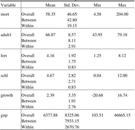
Following section 4, we concentrate on the endogenous variables for which we have observable statistics: fertility, educational attainment, and growth. The data are averages forfive year periods between 1960 and 1990. Variables corresponding to child mortality, adult longevity, fertility, and growth are taken from the World Bank’s World Development Indicators — 1999. These are, respectively: child mortality rate before 1 year (mort), life expectancy conditional on survival to
17The behavior of population in the second half of the twentieth century is also consistent with the discussion in
1 year (adult1), total fertility rate (f ert), and growth rate of the real GNP per capita (growth). Educational attainment is measured by the average schooling in the population aged 25 and above (schl), from the Barro and Lee data set (see Barro and Lee, 1993). The sample is restricted only to countries for which data is available for all the variables and years. This leaves us 71 countries and 7 points in time, which gives a total of 497 observations. Summary statistics for the relevant variables are presented in Table 4. Appendix B describes the data in more detail, and enumerates the countries included in the sample.
Thefirst order conditions for the individual problem implicitly give a set of reduced form equa-tions that express fertility, education, and growth as funcequa-tions of child mortality, adult longevity, and the other exogenous variables:
f ert = f(mort, adult1, X), schl = g(mort, adult1, X), and
growth = q(mort, adult1, X),
where X denotes all other exogenous variables apart from child mortality and adult longevity. Our strategy, in contrast with the traditional empirical growth literature, is to take the model seriously and estimate these reduced form equations. Apart from the life expectancy variables, the only exogenous factors in our model are related to tastes (parameters of the utility function) and technology (parameters of the production functions). To account for shifts in these exogenous variables across countries, we use country fixed effects, so that any systematic difference due to culture, religion, and technology is washed away. Also, to account for possible technological development or absorption through time, we include time dummies.
The issue of exogeneity of the life expectancy gains becomes extremely important here. To control for the changes in life expectancy that are simply a consequence of economic development, we include the natural logarithm of the real GNP per capita (lngnp) in the reduced forms above. This will isolate the changes due to life expectancy, from those directly attributable to development and to behavioral changes induced by increased in income.
With these considerations in mind, the basic specification of our empirical model is given by the following system of seemingly unrelated regressions:
f ertit = βf0+βf1mortit+βf2adult1it+βf3lngnpit+αfi +α f t +εit, schlit = βs0+β1smortit+βs2adult1it+βs3lngnpit+αis+αst+υit, and growthit = βg0+βg1mortit+βg2adult1it+βg3lngnpit+αgi +α