Title: Financial Guarantees in Brazilian Life Insurance and Pension Plans
Track:
Life Insurance
Authors’ Information:
Name: António Simões-Pereira
Title: PhD
Affiliation: F&C Portugal
Full Adress: Av. Jose Malhoa, Lote 1686 1070-157 Lisbon Portugal
Phone: (351) 21 0033247
Fax: (351) 21 0033239
Email:
antonio.pereira@fandc.com
Last name for indexing and correspondence: Simões-Pereira
Name: William Eid Junior
Title: PhD
Affiliation: EAESP / FGV - Escola de Administração de Empresas de São Paulo da
Fundação Getúlio Vargas
Full Adress: Av. Nove de Julho 2029 01313 902 Sao Paulo Brazil
Phone: (55) 11 3281 7994
Fax: (55) 11 3284 1789
Email:
weid@fgvsp.br
Last name for indexing and correspondence: Eid Jr
Financial Guarantees in Brazilian Life Insurance
and Pension Plans
November 2005
Abstract
Recently regulated Brazilian life and pension products offer a benefit structure composed of minimum guaranteed annual rate, inflation adjust-ment according to a price index and participation on an investadjust-ment fund performance. We present a valuation model for these products. We es-tablish a fair condition relationship between minimum guarantees and participation rates, and explore its behavior over a space of maturities, interest rates, and also fund and price index volatilities and correlation. Besides consistency to reference models, we found that the effect of the fund volatility is conditioned to the price index volatility level and the correlation between them.
1
Introduction
Deregulation in the financial and insurance industry during the past decades put life insurance products in direct competition with mutual funds and pension funds, for the savings market. Faced with a new fierce competitive environment, life insurance companies started to add some financial guarantees to their tra-ditional products in order to attract a bigger slice of this huge market. Capital guarantees, minimum annual guaranteed rates, participation on the company results or on specific equity or bond funds returns, early surrender as well as loans against the policy, are some typical examples of financial options that were attached to life insurance products and consequently transformed the liability nature of this industry. Mostly launched between the mid eighties and mid nineties, these options started to be issued at a considerably higher interest rate world. As a consequence they were very cheap, not even considered for pricing, which was ordinarily taken using quite conservative actuarial rates. From mid to late nineties on, interest rates decreased and of course those old cheap liabil-ities which had not even been priced, suddenly became valuablein the money
options. The need for market value turned increasingly evident, since the valu-ation of embedded options became crucial to an assessment of the risk of these products. Several models have been developed since then, identifying and eval-uating these embedded options, like [3], [4],[6] and many others. These models
use financial economics tools to identify and evaluate the options embedded in the products. They provide a guideline to the pricing of these products since they establish, in a very simple way, the price limits that keep the contracts under fair conditions. Normally not considering actuarial risks, their method invariably consists of finding the set of pairs of minimum guarantees and partic-ipation rates, implied by a fairness condition, and to track their behavior under the change of state variables, mainly interest rates and asset volatility. The main findings provided by these models are:
- An inverse relationship between minimum guarantees and participation rates;
- Contract values increase as a result of interest rates reduction;
- In the absence of credit risk, the participation rates are inversely related to the asset volatility;
- Contract values have relatively low sensibility to the correlation between interest rates and asset returns.
In this paper, we develop a simple model applied to Brazilian products, following the same methodology. The main difference to be noticed is the inflation adjust-ment. In this sense we try to investigate the effects of an inflation adjustment to the minimum guarantee on the behavior of fair participation rates.
In the following section we develop the equations of the contracts and define a fair condition. In section 3, we develop the valuation model based on a change of numeraire technique. Then, Section 4 shows the main results comparing them to the above main findings and presenting the effects of new variables. The last section concludes, discusses about the limits of the model and suggest some paths for future research.
2
New Brazilian Life and Pension Products
L(P)MGP - Life (Pension) with Minimum Guarantee and Performance1 were regulated in early 2003 [12]. They differ from traditional Brazilian life insur-ance products, mainly by the segregated character of the assets. In fact, the participation rate is measured on the return of a perfectly defined portfolio, called Specific Investment Fund2. Premiums can be paid either as unique
ini-tial sums or by periodic payments or even at arbitrary amounts and times at policyholder’s whim. Benefits can be paid either as maturity lump-sums or in the form of annuities which, in their turn, can be temporary, life, and so on. Apart from this benefit structure, these products offer the possibility of early surrender as well as the transfer from life to pension plans of the same type, and vice versa. Also, the participation rate can vary in an increasing way, provided
1
Which is called V(P)RGP - Vida (Plano) com Remunera¸c˜ao Garantida e Performance 2
it is pre-established in the contract. Adding some variations on the way manage-ment expenses can be paid, we face a highly complex product to model. In face of such complexity we chose to establish a simpler treatable generic contract, which will be our valuation object.
2.1
A generic simplified contract
Assumptions:
- Actuarial risks are not considered.
- Premium is unique and paid at the beginning of the contract.
- Benefit is paid in a lump-sum at timeT, the maturity of the contract.
- This generic contract does not allow for early surrender.
- Underwriting and management expenses are not considered.
- Reversion of performance participation to the reserve account is considered to be made at maturity only.
Taking this simplified framework, a policyholder pays a premium X at the momentt= 0 to the insurance company, who invests it in a specific investment fundS. A reserve accountM 3is created in the liability side of the balance sheet
and represents at every moment theminimumbenefit owed to the policyholder if she surrendered at that given moment. The excess result Ei at the end of
each monthiis defined as:
Ei =Mi−1.[(1 +δi)−(1 +gm)(1 +θi)] (1)
where:
- E, is the excess return of S over the minimum guarantee adjusted for inflation.
- Mi−1, is the reserve account at the end of the previous month.
- δi is the return ofS during the period (i−1, i)
- gm, is the monthly equivalent minimum guaranteed rate.
- θiis the inflation rate during the period (i−1, i) measured as the variation
of the price indexIduring that period.
When positive, a shareα.Eiof the monthly excess return is credited in a second
liability account named Provision for Excess Results which we denote byB 4.
The complement of that share, (1−α).Ei is credited in an equity account C
3
This account is named Provis˜ao Matem´atica de Benef´ıcios a Conceder 4
of the company. When negative, it means the return ofS won’t be enough to pay the minimum guarantee, i.e. it is below the minimum adjusted guarantee. The difference must be covered by the balances ofB and Cin the proportions
α and (1−α) respectively. In case the balance of B is not enough to cover
α.Ei, the difference will also be covered by the equity accountC, regarding that
it will be repaid by future positive balances ofB, capitalized by the return of
S. The balance of B account is periodically reverted to the reserve account
M. Although not mandatory on a periodic basis, the reversion periodicity cannot exceed five consecutive years. As stated in the last assumption, we restrict our analysis to the case of maturity reversion. Meanwhile, for the sake of understanding the dynamics of the different accounts let us assume for now that reversion is made on an annual basis.
Let us now define A, the policyholder account, whose balance is the sum of the balances ofM andE. Whenever reversion takes place the balance of A
equals the balance ofM. From that moment on, until the next reversion, M
evolves according to minimum adjusted guaranteed rate and E, according to the excess results obtained every month. Immediately after every reversion, the balance ofE is, of course, zero. So, assuming the reversion at the end of each yeart, it is not difficult to conclude that:
At=At−1(1 +g)(1 +θt) +α.[Et]+ (2)
Ct = Ct−1(1 +δt) + (1−α).[Et]+−[Et]−
= Ct−1(1 +δt) + [Et]+−α.[Et]+−[Et]− (3)
where
- Et=Mt−1[(1 +δt)−(1 +g)(1 +θt)].
- [Et]+=max[Et,0]
- [Et]−=max[−Et,0].
- δtis the return ofS during the interval [t−1, t].
- g is the minimum annual guaranteed rate.
- θtis the inflation rate, between (t−1) andt.
The options involved are clearly shown. Considering now that reversion takes place only at maturityT, we can say that:
AT =X.(1 +g)T.
IT
I0
+α.[ET]+ (4)
Another way to expressAT in which we can clearly see the exchange of options
between insurance company and policyholder, is:
AT =X T
Y
t=1
(1 +δt)−(1−α)[ET]++ [ET]− (6)
One sees immediately that the policyholder is long a put option on the per-formance. This put is indeed the minimum adjusted guarantee; short on a (1−α) percentage of a call option on the performance. The insurance company is short the same put option and long the same percentage on the performance. Summing up 5 and 6 we obtain:
AT +CT =X T
Y
t=1
(1 +δt) =XT (7)
In continuous time, we can write forA:
AT =X.
(
egT.IT I0 +α
·S
T
S0 −e gT.IT
I0
¸+)
(8)
3
Fair Contracts
The so called Contribution Principle, states that benefits must be shared be-tween the policyholder and the insurance company in the proportion of the contributions made. According to this principle, a contract is said to be fair when the present value of the premium equals the present value of the expected benefits. It must be stressed that this present value calculation implies an ex-pectation calculated under an equivalent martingale measure. Following [9] we can write that:
V0(AT) =V0(X) (9)
V0(CT) = 0 (10)
WhereV0 is merely a present value operator. Thus,
V0(AT)
V0(X)
= 1 (11)
Considering that the initial premium X is evaluated at t = 0, we can write
V0(X) =X:
V0( AT
X ) = 1 (12)
V0(AT
X ) = 1 =e
−rTEQ
(
egT.IT I0
+α
·
S(T)
S(0) −e
gT.IT
I0
¸+)
(13)
whereEQ is an expectation under the equivalent martingale measure, andris
the risk free short rate of interest.
4
A Simple Valuation Model
AT/X can then be seen as the contract function for an European derivative
that, att = 0, has value 1. This means we face an inverted problem, like the well known case of implied volatilities. In fact we want to find pairs (g, α) that satisfy that fairness condition. We use the notation Υ for this contract function. Thus, we have:
Υ(T) = (
egT.IT
I0
+α
·S(T)
S(0) −e
gT.IT
I0
¸+)
(14)
and then, we designate Ψ(t,Υ) the price process of the contract, which has value 1 att = 0. To obtain Ψ(t) we follow closely [1], using a change of numeraire technique to evaluate options which strike price is a function of a price index. To start with, we consider an economy with the following assumptions:
- A temporal horizon [0, T].
- There are no transaction costs and every security is considered perfectly divisible.
- Short selling is allowed.
- Trade is continuous.
- Real interest rateRis assumed to be constant.
- There are no opportunities of arbitrage.
- Uncertainty is represented by a probability space (Ω,F, P), where Ω is the set of all possible states of natures,F is theσ-algebra of the subsets of Ω andP is a probability measure. Information is revealed through time by the filtration F ={Ft, t∈[0, T]}, consisting in an increasing sequence of
σ-algebras, i.e.,Fs⊂ Ftfort≥s. Att= 0 there is no information
avail-able and at momentT uncertainty ceases, since all information relative to the temporal horizon is already available [11].
At these conditions the value of an european derivative can be expressed by:
Ψ(t,Υ(T)) =U(t)EQU t
· Υ(T)
U(T) ¸
whereQU is the probability measure induced by the numeraireU. Numeraire is
any tradeable asset that pays no dividends, at least during the temporal horizon considered. It is the asset in terms of which other asset values are expressed. In these more general terms, we can express 13 as:
U(0)EQU t
( 1
U(T) "
egT.IT I0 +α
·S(T)
S(0) −e
gT.IT
I0
¸+#)
= 1 (16)
For the sake of clearness we can divide the contract function in two parts: The guarantee termegT.IT
I0; And the option term, h
S(T) S(0) −e
gT.IT I0
i+
. We take first the later, and denote its contract function by Φ:
Φ =max[S(T)
S(0) −e
gTI(T),0] (17)
without any loss of generality, we can assume that:
S(0) = 1
I(0) = 1
Following [1], the underlying assetS, is assumed to evolve according to a geo-metric brownian motion like:
dS(t) =S(t)µdt+S(t)σ′
SdW (18)
or,
dS(t) =S(t)rdt+S(t)σ′
SdWQ (19)
under a risk neutral measureQ[2]. On its turn, based on [8] and [7], we consider the following process for the price index,I:
dI(t) =I(t)(r−R)dt+I(t)σ′
IdWQ (20)
also under the measureQ. In these processes,rrepresents the nominal risk free short term interest rate,Ris real interest rate anddWQa vector of two standard
Wiener processes defined on the probability space (Ω,F, P), constituting the two sources of uncertainty of this economy:
µ
dw1 dw2
σS andσI are two column vectors:
µ
σS1(I1) σS2(I2)
where σ2
Sj(Ij) represents the variance ofS (orI), per unit of time, originated
by the source of uncertainty j = 1,2. As we can see, the strike price of the option is a function of the price indexI. At every momentt, this exercise price can be expressed by:
K(t) =egTI(t)
To evaluate this option we use a change of numeraire technique. A natural candidate for numeraire would be the price indexI, itself. However, I is not a tradeable asset and, as such, it cannot play that role. Notwithstanding, consid-ering a constant real interest rateR, we can define an assetU:
U(t) =eRt.I(t) (21)
which stands for a deposit that pays a constant real interest rate plus inflation, as measured by the price indexI. By direct application of Ito’s Lemma, the processU(t) can be expressed by:
dU(t) =U(t).rdt+U(t)σIdWQ (22)
U(t) is then a tradeable asset that pays no dividends and, this being so, it can be chosen for numeraire. The process value of the option can then be written as:
Π(t,Φ(T)) =U(t)EQU
t [maxZ(T)−K(T),0] (23)
where:
- Π(t,Φ) is the process value for the option.
- Φ(T) is the option’s contract function.
- QU is the equivalent martingale measure induced by the numeraireU.
- Z(T) =US((TT)).
- K(T) = egTU(IT(T))=e(g−R)T, considering thatI(T) =U(T)e−RT.
By Ito’s Lemma and the Main Theorem on [1], we see that Z has null drift underQU:
dZ(t) =Z(t)(σS−σI)dWU (24)
Π(t,Φ) can then be calculated by direct application of Black-Scholes for a call option with strike priceKon an asset with scalar volatility expressed by5:
5
δZ =kσ′S−σI′k=
q
kσSk2+kσIk2−2σSσ′I =
q
δ2
S+δ2I−2ρδSδI
in a normalized economy with a zero risk free rate of interest, since UU((tt)) = 1. In these terms, the value of this option can be written as:
Π(t,Φ) =U(t){Z(t)N[d1]−KN[d2]} (25)
with:
d1=
1
δZ.
√ T −t
½
ln
µZ(t)
K
¶ +1
2δ
2 Z(T−t)
¾
d2=d1−δZ
√ T−t
substituting the expressions forZ(t) andK, and taking S(0) = I(0) = 1, we obtain:
Π(t,Φ) =S(t)N[d1]−I(t)e−R(T−t)egT S(0)
I(0)N[d2] (26) with
d1= 1 δZ
p (T −t)
½
ln
µ
S(t)I(0)
I(t)S(0)egT
¶ +
µ
R+1 2δ
2 Z
¶ (T−t)
¾
(27)
d2=d1−δZ
√
T−t (28)
where, as already seen,
δZ=
q
δ2
S+δI2−2ρδSδI (29)
But the contract does not resume to the call itself. In fact, taking 16, we have:
Ψ(t,Υ(T)) =U(t)EQU t
½
e(g−R)TU(T)
U(T)+α.max[Z(T)−K(T),0] ¾
(30)
or,
Ψ(0,Υ(T)) = U(0)EQU t
n
e(g−R)To+
+ U(0)EQU
t {α.max[Z(T)−K(T),0]}= 1 (31)
substituting Π(0,Φ(T)) for the option term:
Ψ(0,Υ(T)) =U(0)e(g−R)T+α.Π(0,Φ(T)) = 1 (32)
e(g−R)T +α.£
N(d1)−eg−RN(d2)¤= 1 (33)
with d1 e d2 as expressed in 27 e 28 respectively. That’s precisely under this
closed solution that we will find pairs ofgandαwhich satisfy the fair condition of the contract, Ψ(0,Υ(T)) = 1. Before we proceed, three observations must be made. First, the process we used for the price index is based on an analogy established by [8] and [7] from the Garman and Kholhagen (1983) model, where the process of an exchange rate is of the same nature of an equity that pays a constant dividend yield. Second, the equivalent martingale measures were not explicit because we simply do not need them in the Black-Scholes framework. Third, notice the market is complete, since the depositU does not exclude the existence of the bank accountB that pays nominal risk free interest rate,r. In fact, we have two sources of uncertainty, two risky assets,SandU, and the risk free asset,B.
5
Main results
In quite general terms, we want to find pairs (g, α) that satisfy:
F(g, α, T;δS, ρ, δI, R) = 0 (34)
where the functionalF is a simplified representation for 33.
5.1
Defining a Universe
Through 33 equation above we find (g, α) keeping the remaining variables con-stant. First, we distinguish the contract parameters,g,αandT, over which the company has some control, from the external variables,δS,δI andρ. Of course,
in a way, the company has some control over the asset volatility since it can choose the asset allocation ofS, and consequently the same forρ. Second, based either in regulation statements or in historical series, we establish a universe for each parameter and external variable.
- g has a regulated cap of 6%. For our purposes, we chose
{0%,1%,2%,3%,4%,5%,6%}
.
- α, is considered in the interval{0,1}.
- T is, for a unique maturity reversion, limited to 5 years, by regulation. Anyway, we assume higher maturities in order to evaluate the effects ofT
- δS is made to variate in the set ∆S = {20%,30%,40%,50%,60%,70%}
which is based on a series of annualized IBOVESPA daily volatilities over five year windows6 between 1989 and 1998.
- δI, was observed over monthly variations of the price index IGP −M,
between June 1989 and November 2003, also on five year windows. Given the difference in values for the periods before and after Real Plan, we chose two separate universes, so that we can evaluate the effects of changingδI
on both regimes: pre-Real Plan ∆I1 = {60%,50%,20%} and post-Real
Plan ∆I2 ={2%,3%,4%}.
- The universe forρwas established taking parallel series of IBOVESPA and IGP-M monthly returns from June 1989 to November 2003, taking their maximum, minimum and average values, over pre and post Real Plan:
ρ={10%,30%,60%,80%}
- Finally, real interest rates were taken from [10] and [5]. The universe is Ψ ={3%,6%,10%,15%}.
For each parameter or variable universe, a reference value was defined, as the value to be kept constant when any other parameter or variable variation is at stake. So, we have:
Reference Set
T (years) 5
Volatility S 40% Volatility I 3% Correlation 30%
R 6%
g 3%
Table 1: Reference set
Using the Excel Goal-Seek numerical search algorithm within a macro for a table of numbers, we simply constructed the matrices:
αg,Q=α(g, Q)Qr
which is F explicit in α. Each of these matrices shows fair α for eachg and a second argumentQ, keeping the rest of the arguments Q at their reference values.
6
5.2
Main Findings
- The minimum guaranteeg is bounded by the real interest rate. In fact, if g > R, the guarantee will be above 1, keeping the participation rate negative, meaning that the insurance company will have a (1 +α) over the excess result. In this case, the company would promise an above risk free rate of interest on a no risk product and then should be compensated, by a long position in a share of a call. Of course one needs to notice that this boundary is made in terms of the real rate and that constitutes a limitation of the model.
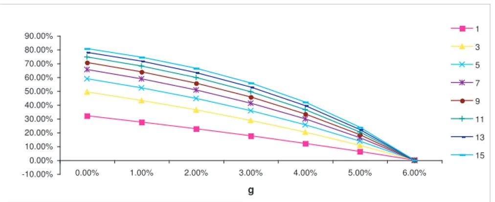
- An inverse relationship between minimum guaranteed rate and participa-tion rate is clear from the model. Figure 1 illustrates this relaparticipa-tionship, for different maturities. This kind of graph is meant to be a pricing guide, since it relates the three contract parameters. Higher minimum guarantee implies a lower participation. In fact, as the insured gets a higher guaran-teed rate, she will accept a lower participation. Guarantees are normally issued below risk free interest rates, the participation rate making up the difference to get a fair return, i.e., a return that compensates the policy-holder for the risk she takes. When no credit risk is considered as is the case, fair return means risk free interest rate.
-10.00% 0.00% 10.00% 20.00% 30.00% 40.00% 50.00% 60.00% 70.00% 80.00% 90.00%
0.00% 1.00% 2.00% 3.00% 4.00% 5.00% 6.00%
g
1
3
5
7
9
11
13
15
Figure 1: Participationα(alpha) as function ofg, varyingT. R=6%,δS= 40%,δI= 3%,
ρ= 30%.
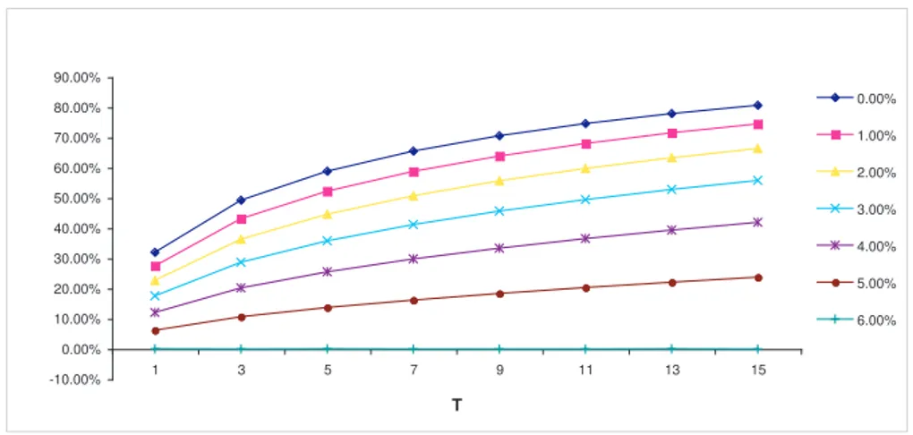
- Higher maturities allow for higher levels of participation. In fact, higherT
implies a lower value guarantee term and, to get the fair condition, a higher participation is then required. Notice that the option value increases with
T, but this effect is clearly dominated by the effect on the guarantee term. Figure 2 shows fair contract curves for each maturity, considering reference values for external variables.
- For a giveng, the effects ofδS, δI and ρon the level of participation are
-10.00% 0.00% 10.00% 20.00% 30.00% 40.00% 50.00% 60.00% 70.00% 80.00% 90.00%
1 3 5 7 9 11 13 15
T
0.00%
1.00%
2.00%
3.00%
4.00%
5.00%
6.00%
Figure 2: Participationα(alpha) as function ofT, varyingg.R= 6%,δS= 40%,δI= 3%,
ρ= 30%.
dα dδS
=−
∂F ∂δS ∂F ∂α
(35)
where
∂F ∂δS
= ∂F
∂δZ
.∂δZ ∂δS
Substituting Eq.33 for F, it is immediate to see that ∂F
∂α is the value of
an option and, as such, is non negative. Also, ∂δ∂FZ has positive sign, since the option value increases with its underlying asset’s volatility. Then, the sign of Eq.35 will be negative when:
∂δZ
∂δS
>0
It is easy to conclude that, forρ >0:
∂δZ
∂δS
>0⇔ δδS
I
> ρ
Then, forρ >0, the participation rate decreases withδS if δδSI > ρ. Using
the same reasoning forδI, we obtain:
∂δZ
∂δI
>0⇔ δδI
S
> ρ
Then, forρ >0, the participation rate decreases if δI
δS > ρ. Of course, if
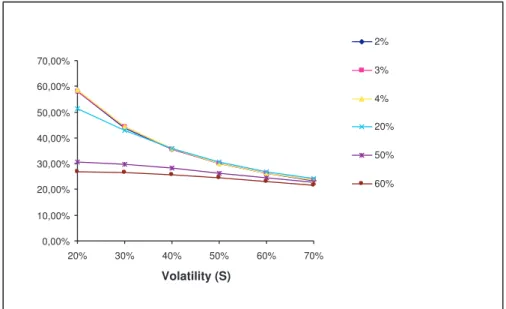
of αwith δS for all considered levels of δI keeping the correlation at its
reference level, 30%. It is easy to see the lower influence of δS on α, for
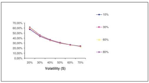
higher levels ofδI. Also, Figure 4 shows a decreasingα(δS), forδI = 3%,
not being significantly affected across all considered levels of ρ. Figure 5 illustrates precisely the same relationship, but now keepingδI at its Pre
Real reference level of 50%. We can see αincreasing to the point where
δS =ρ.δI, when ρ = 80% orρ= 60% . For lower levels of δI, as is the
case for Post Real Plan,αshows a decreasing behaviour withδS.
0,00% 10,00% 20,00% 30,00% 40,00% 50,00% 60,00% 70,00%
20% 30% 40% 50% 60% 70%
Volatility (S)
2%
3%
4%
20%
50%
60%
Figure 3: Participationα (alpha) as function of δS, varying δI. T = 5 years, g = 3%,
R= 6%,ρ= 30%.
The analysis forδI is entirely analogous, although one must pay attention
to the universes ofδS and δI. Forρ, we have:
dα dρ =−
∂F ∂ρ ∂F ∂α
and
∂δZ
∂ρ = −δSδI
δZ
0,00% 10,00% 20,00% 30,00% 40,00% 50,00% 60,00% 70,00%
20% 30% 40% 50% 60% 70%
Volatility (S)
10%
30%
60%
80%
Figure 4:Participationα(alpha) as function ofδS, varyingρ.T = 5 years,g= 3%,R= 6%,
δI= 3%.
|∂α∂ρ|
|∂α ∂δS|
= δSδI
|δS−ρδI|
and analogously,
|∂α ∂ρ|
|∂α ∂δS|
= δSδI
|δS−ρδI|
Then, it is immediate: when negative, ρ has a smaller influence on α, compared to δS and δI. However, when positive, its influence on the
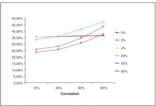
participation depends on the levels ofδS andδI. 6 showsα(ρ) practically
constant for lower Post Real Plan levels ofδI, and increasing for higher
Pre Real Plan δI. Even a high correlation does not appear to affect α
providedδI is low enough.
Summing up, we could see the intimate relationship among these variables. When the volatility of its underlying asset increases, the value of the option also increases.
0,00% 5,00% 10,00% 15,00% 20,00% 25,00% 30,00% 35,00% 40,00% 45,00% 50,00%
20% 30% 40% 50% 60% 70%
Volatility (S)
10%
30%
60%
80%
Figure 5:Participationα(alpha) as function ofδS, varyingρ.T = 5 years,g= 3%,R= 6%,
δI= 50%.
is a normalized asset entity, which volatility depends on the volatilities of
S,Ias well as their correlation. For a given investment fund volatilityS, the effect of the volatility ofI, depends first on its level. Then this first effect can be expanded or amortized depending on the correlation. Higher positive correlation toI, amortizes the effect ofδIon the aggregate
volatil-ity, diminishing then the risk and possibly increasing the participation rate to the policyholder. On the contrary, negative correlation toδI expands
the effect of δI on the aggregate volatility, and then causes lower
par-ticipation to the policyholder. All these aspects are therefore intimately related.
6
Conclusions
The model proposed above shows good coherence with reference models’ results. It shows also the importance of the relationship among asset volatility, price in-dex volatility and their correlation, in determining fair levels of participation rates. We found that the effects of asset volatility on the fair level of partici-pation rate are conditional to the volatility level of the index price and to the their correlation.
0,00% 5,00% 10,00% 15,00% 20,00% 25,00% 30,00% 35,00% 40,00% 45,00% 50,00%
10% 30% 60% 80%
Correlation
2%
3%
4%
20%
50%
60%
Figure 6: Participationα (alpha) as function of ρ, varying δI. g = 3%, T = 5 years,
δS= 40%ρ.
generic ideal product full of simplifications. Of course, early redemptions, rever-sions, periodic premiums and annuities will add a lot of complexity to the model. Also, the model assumptions put some simplification to the problem: constant real interest rates, geometric brownian motions both to the asset and price in-dex dynamics. These are, of course limitations that clearly indicate future field of research. Notwithstanding, the use of this simplified structure will certainly be helpful in binding the price process of life insurance and pension products, precisely in terms of identifying financial sources of risk formerly treated in a deterministic and sometimes, overly conservative way.
References
[1] S. Benninga and Z. Bjørk, T.and Wiener. On the use of numeraires in option pricing. The Journal of Derivatives, pages 43–58, Winter 2002.
[2] T. Bjørk. Arbitrage Theory in Continuous Time. Oxford University Press, 1998.
[4] E. Briys and F. De Varenne. Life insurance in a contingent claim frame-work: Pricing and regulatory implications. The Geneva Papers on Risk and Insurance Theory, (19):53–72, 1994.
[5] M.G.P. Garcia. Brazil in the 21 century: How to escape the high real interest trap? Technical report, Pontifcia Universidade Catlica - Rio de Janeiro, January 2004.
[6] A. Grosen and P.L. Jørgensen. Fair valuation of life insurance liabilities.
Insurance: Mathematics and Economics, 26(1):37–57, 2000.
[7] R.A. Jarrow and Y. Yildirim. Pricing treasury inflation protected securi-ties and related derivatives using an hjm model. Working paper, Johnson Graduate School of Management, Cornell University, and School of Man-agement, Syracuse University, Syracuse, Ithaca, N.Y., February 2002.
[8] Y. Landskroner and A. Raviv. Pricing inflation-indexed and foreign-currency linked convertible bonds with credit risk. Working paper, School of Business Administration, Hebrew University of Jerusalem, Israel,and Stern School of Business, New York University, N.Y., March 2003.
[9] K.R. Miltersen and S.-A. Persson. Guaranteed investment contracts: Dis-tributed and undisDis-tributed excess returns. Working paper, Institute of Fi-nance and Management Science, Norwegian School of Economics and Busi-ness Administration, Hellevian 30, N-5045 Bergen Norway, 2000. Forth-coming in Scandinavian Actuarial Journal.
[10] P.C. Miranda and M.K. Moinhos. Taxa de juros de equilbrio: Uma abor-dagem mltipla. Working Paper 66, Banco Central do Brasil, Fevereiro 2003.
[11] S.-A. Persson and K.K. Aase. Pricing of unit-linked life insurance policies.
Scandinavian Actuarial Journal, (1):26–52, 1994.