Submitted 29 March 2015
Accepted 11 May 2015
Published7 July 2015
Corresponding authors Xinping Cui, xinping.cui@ucr.edu Kang Ning, ningkang@qibebt.ac.cn
Academic editor Yong Wang
Additional Information and Declarations can be found on page 23
DOI10.7717/peerj.993 Copyright 2015 Wang et al.
Distributed under
Creative Commons CC-BY 4.0 OPEN ACCESS
MetaBoot: a machine learning
framework of taxonomical biomarker
discovery for di
ff
erent microbial
communities based on metagenomic data
Xiaojun Wang1,2, Xiaoquan Su1,3, Xinping Cui1,4and Kang Ning1,2,3 1Bioinformatics Group of Single Cell Center, Shandong Key Laboratory of Energy Genetics and
CAS Key Laboratory of Biofuels, Qingdao Institute of Bioenergy and Bioprocess Technology, Chinese Academy of Sciences, Qingdao, Shandong Province, People’s Republic of China
2University of Chinese Academy of Sciences, Beijing, People’s Republic of China 3CUDA Research Center, Qingdao Institute of Bioenergy and Bioprocess Technology,
Chinese Academy of Sciences, Qingdao, Shandong Province, People’s Republic of China
4Department of Statistics, University of California, Riverside, CA, USA
ABSTRACT
As more than 90% of species in a microbial community could not be isolated and cultivated, the metagenomic methods have become one of the most important methods to analyze microbial community as a whole. With the fast accumulation of metagenomic samples and the advance of next-generation sequencing techniques, it is now possible to qualitatively and quantitatively assess all taxa (features) in a microbial community. A set of taxa with presence/absence or their different abundances could potentially be used as taxonomical biomarkers for identification of the corresponding microbial community’s phenotype. Though there exist some bioinformatics methods for metagenomic biomarker discovery, current methods are not robust, accurate and fast enough at selection of non-redundant biomarkers for prediction of microbial community’s phenotype. In this study, we have proposed a novel method, MetaBoot, that combines the techniques of mRMR (minimal redundancy maximal relevance) and bootstrapping, for discover of non-redundant biomarkers for microbial communities through mining of metagenomic data. MetaBoot has been tested and compared with other methods on well-designed simulated datasets considering normal and gamma distribution as well as publicly available metagenomic datasets. Results have shown that MetaBoot was robust across datasets of varied complexity and taxonomical distribution patterns and could also select discriminative biomarkers with quite high accuracy and biological consistency. Thus, MetaBoot is suitable for robustly and accurately discover taxonomical biomarkers for different microbial communities.
Subjects Bioinformatics
INTRODUCTION
The approximate estimation of microbial cells on earth is 1030(Proctor, 1994), which is huge, and a large number of novel genes with useful functions might be contained within the genomes of these unknown communities of microbes. However, it was estimated that more than 90% of species in the microbial communities are unknown and uncultivable (Jurkowski, Reid & Labov, 2007). Therefore, the traditional processes for isolation and cultivation of microbes are not applicable for the analyses of many microbial communities. Based on the development of Next Generation Sequencing (NGS), the metagenomic method become one of the important methods that could provide direct access to genomes of as-yet-uncultivated microorganisms in native environments (Eisen, 2007). Metagenomics makes it possible to better understand microbial diversity as well as their functions. Metagenomics has become an increasingly popular research area when its diverse and multiplicity of metagenomics and its potential applications in environmental sciences, bioenergy and human health is considered.
One of the most broadly applicable and successful means of translating molecular and genomic data into applications such as clinical practice (Segata et al., 2011) and environmental monitoring (Lam & Gray, 2003) is the identification of biomarkers. Comparisons among different types of tissues or samples have highlighted the importance of detecting novel subtypes of a disease or determining the subtype of a new sample (Golub et al., 1999;Tothill et al., 2008). In any genomic dataset, identifying the most biologically informative features which can differentiate two or more sets of samples remains an obstacle, and for metagenomic biomarkers this is particularly true.
Other than the challenges associated with high-dimensional data which includes different meta data or data type, metagenomic analysis additionally presented their own specific issues, including sequencing errors, chimeric reads (Swan et al., 2002;Wooley & Ye, 2010) and complex underlying biology (multiple species and their uniqueness, relative abundances, complex functions, etc.). Remarkable inter-subject variability would usually present a profound property of many microbial communities as well, which has made biomarker identification a big hurdle. For instance, both environmental and human microbiomes might be subjected to a long tail distribution of rare organisms (Liao et al., 2011;Pedr´os-Ali´o, 2006). Therefore, robust and efficient bioinformatics tools that could ensure the reproducibility of biomarker identification from metagenomic data, which is crucial for its applications, are needed. Further, as mentioned inSegata et al. (2011), elucidating the biological consistency and roles of selected biomarker, especially non-redundant biomarkers, is a crucial step to understand the underlying mechanisms of community–community or host-community interactions.
comparing different communities. TreeClimber (Schloss & Handelsman, 2006b), UniFrac (Lozupone & Knight, 2005) and Meta-Storms (Su, Xu & Ning, 2012) compare sets of metagenomics in a phylogenetic context. Secondly, there are tools for comparing two sets of samples. MEGAN (Huson et al., 2007) is a metagenomic analysis tool providing a graphical interface that allows users to compare the taxonomic composition of samples, with additions for phylogenetic comparisons and statistical analyses. MEGAN, however, can only compare single pairs of metagenomic samples, which is also the case with STAMP (Parks & Beiko, 2010). Thirdly, statistical model based methods were developed for the comparison of samples. MG-RAST (Meyer et al., 2008), ShotgunFunctionalizeR (Kristiansson, Hugenholtz & Dalevi, 2009), Mothur (Schloss et al., 2009) and METAREP (Goll et al., 2010) all compare metagenomic samples through standard statistical tests. However, none of these methods directly identify biological features responsible for group relationships (Gower, 1966).
The identification of biomarkers for metagenomic data could illustrate the reason for metagenomic sample differences. There are two general approaches for metagenomic biomarker discovery: bottom-up and top-down. The bottom-up method is the one that tested each taxa and selected ones that would led to the variations between groups. Typical bottom-up methods include Wilcoxon rank-sum test (Wilcoxon) (Bauer, 1972). The top-down method is based on statistical analysis of the overall distribution of taxon in the metagenomic samples. Currently, Metastats (White, Nagarajan & Pop, 2009) and LEfSe (Segata et al., 2011) are the only two available methods that explicitly apply statistical assessment of metagenomic difference for metagenomic biomarker discovery. LEfSe further considered biological relevance, biological consistency and effect size estimation of predicted biomarkers. As pointed out by LEfSe (Segata et al., 2011), to ensure reproducibility of biomarker identification from metagenomic data, robust statistical tools are needed, which is also critical for clinical applications. However, none of the aforementioned two methods have addressed the issue of robustness. In addition, redundancy is a serious issue for metagenomic data analysis, especially for biomarker discovery. Taxonomically, as microbial community is dynamic, it is very common that there exist many similar strains as well as multiple similar mutants of the same strain. However, to maximize the power of biomarkers for clinical diagnostic application, it is desirable to find biomarkers that are both distinguishable and representative. Therefore, biomarkers from the same strain and its mutants or from similar strains are considered as redundant biomarkers since they contain similar genetic and/or clinical information. Note that redundancy in biomarker discovery from gene expression data is less of an issue in that even though two or more genes might be similar, they might play significantly different roles in the biological system (biological importance). Additionally, the evolutionary relationship among similar genes might not be that close enough to treat them as the redundant biomarker.
structure of the microbial community, and then summarized such property for biomarker identification. The MetaBoot framework is based on taxonomical profiles generated from the microbial community’s 16S rRNA gene sequences. It selects discriminative features as candidate features through bootstrap resampling. This general procedure is simple in principle, yet it is significantly different from previous biomarker discovery methods: the final results would be a set of non-redundant and informative features (genes) selected by mRMR, rather than a complex taxonomy structure or a set of many biologically redundant features. Also, it introduces bootstrap resampling procedure to ensure the robustness and reproducibility.
MetaBoot has been put to the test and compared with other methods on well-designed simulated metagenomic datasets with known biomarkers and realistic taxonomical distribution properties. Results have shown that MetaBoot was robust for biomarker discovery across datasets of varied complexity and taxonomical distribution patterns. On real oral and soil metagenomic datasets, MetaBoot could also select discriminative biomarkers with high specificity and clear biological meaning.
MATERIALS AND METHODS
Data description
Synthetic datasets
We generated three collections of artificial datasets in order to compare MetaBoot with other methods.
Synthetic dataset S1 (normal dataset). To demonstrate the ability of our method to select features with lower redundancy compared with LEfSe, Metastats and Wilcoxon, we built synthetic datasetS1(Fig. 1). DatasetS1includes 2 classes with three subclasses each, and each subclass has 20 samples. For each sample, there are 10 feature groups (with 10 features in each group) for positive biomarkers and 1 feature group (with 900 features) for negative biomarkers. Therefore, there are 1,000 features and 120 samples in total. For each of the 1,000 features, the values is sampled from a Gaussian normal distribution as described in
Fig. 1. DatasetS1has two properties: first, for positive marker groups, features in class 1 and class 2 have clear difference in mean values, and the between-class differences are larger than between-subclass differences. Secondly, there are feature-to-feature variations within the same feature group due to random distribution function. Nevertheless, features within the same feature groups are considered as redundant features in the dataset.
Figure 1 The structure of synthetic datasetS1(dataset with normal distributions).There is a 20(sam-ples)*10(features) matrix in each subclass and positive marker group. And data in each matrix was generated by the normal distribution function (rnormin R) . More specifically, for group 1–5, the mean parameters for subclass 1, 2, 3 were randomly sampled from the vector (11, 12, 13 and 14); while the mean parameters for subclass 4, 5, 6 were randomly sampled from the vector (17, 18, 19 and 20). Data in group 6–10 were generated in a similar way by using these two vectors reversely. The 900 features in negative marker group all had the same mean value of 15. All features had the same standard deviation (sd) parameters.
of gamma distribution than that ofrateparameter, most of the positive markers among subclasses have differentshapeparameter. The biomarkers that could differentiate “class 1” and “class 2” samples were the subject of biomarker identification.
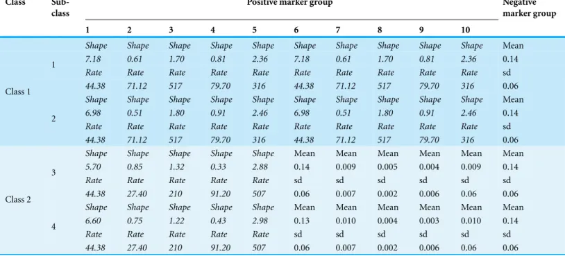
Synthetic dataset S2 (mixture dataset). The detailed parameter settings were shown inTable 1. For positive marker groups 1–5, features in class 1 and class 2 have clear difference inshapevalues. And for positive marker groups 6–10, features in class 1 (gamma distribution) and class 2 (normal distribution) have clear difference inmeanvalues. (The meanandsdvalues of features in class 2 are determined based onmeanandsdvalues from corresponding features in class 2 with gamma distribution.) DatasetS2(mixture dataset) has three properties: first, for positive marker groups, features in class 1 and class 2 have clear difference inshapeormeanvalues, and the between-class differences are larger than between-subclass differences. Secondly, for negative marker groups, there is no difference between classes inmeanvalues. Thirdly, there are feature-to-feature variations within the same feature group due to random distribution function. Nevertheless, features within the same feature groups are considered as redundant features in the datasetS2. The biomarkers that could differentiate “class 1” and “class 2” samples were the subject of biomarker identification.
Synthetic dataset S3 (gamma dataset). The detailed parameter settings were shown in
Table 1 The structure of synthetic dataset S2 (dataset with mixture distributions). In positive marker group, each square is a 25(sam-ples)*10(features) matrix in which each feature was generated by gamma (the red cells) or normal (the green cells) distribution function (generated byrgammaorrnormin R). But in negative marker group, each square is a 25(samples)*900(features) matrix in which each feature was also generated by normal distribution function.
Class
Sub-class
Positive marker group Negative
marker group
1 2 3 4 5 6 7 8 9 10
Shape Shape Shape Shape Shape Shape Shape Shape Shape Shape Mean
7.18 0.61 1.70 0.81 2.36 7.18 0.61 1.70 0.81 2.36 0.14
Rate Rate Rate Rate Rate Rate Rate Rate Rate Rate sd
1
44.38 71.12 517 79.70 316 44.38 71.12 517 79.70 316 0.06
Shape Shape Shape Shape Shape Shape Shape Shape Shape Shape Mean
6.98 0.51 1.80 0.91 2.46 6.98 0.51 1.80 0.91 2.46 0.14
Rate Rate Rate Rate Rate Rate Rate Rate Rate Rate sd
Class 1
2
44.38 71.12 517 79.70 316 44.38 71.12 517 79.70 316 0.06
Shape Shape Shape Shape Shape Mean Mean Mean Mean Mean Mean
5.70 0.85 1.32 0.33 2.88 0.14 0.009 0.005 0.004 0.009 0.14
Rate Rate Rate Rate Rate sd sd sd sd sd sd
3
44.38 27.40 210 91.20 507 0.06 0.007 0.002 0.006 0.06 0.06
Shape Shape Shape Shape Shape Mean Mean Mean Mean Mean Mean
6.60 0.75 1.22 0.43 2.98 0.13 0.010 0.004 0.003 0.010 0.14
Rate Rate Rate Rate Rate sd sd sd sd sd sd
Class 2
4
44.38 27.40 210 91.20 507 0.06 0.007 0.002 0.006 0.06 0.06
groups, features in class 1 and class 2 have clear difference inshapevalues, and the between-class differences are larger than between-subclass differences. Secondly, for negative marker groups, there is no difference between classes inshapevalues. Thirdly, there are feature-to-feature variations within in the same feature group due to random function. Nevertheless, features within the same feature groups are considered as redundant features in the datasetS3. The biomarkers that could differentiate “class 1” and “class 2” samples were the subject of biomarker identification.
Real datasets
Table 2 The structure of synthetic dataset S3 (dataset with gamma distributions). In positive marker group, each square is a 20(sam-ples)*10(features) matrix in which each feature was generated by gamma distribution function (rgammain R). But in negative marker group, each square is a 20(samples)*300(features) matrix in which each feature was also generated by gamma distribution function.
Class
Sub-class
Positive marker group Negative marker
group
1 2 3 4 5 6 7 8 9 10 1 2 3
Shape Shape Shape Shape Shape Shape Shape Shape Shape Shape Shape Shape Shape 7.18 0.61 2.22 1.70 1.29 0.87 0.81 2.56 1.50 1.66 6.20 3.10 0.61 Rate Rate Rate Rate Rate Rate Rate Rate Rate Rate Rate Rate Rate 1
44.38 71.12 33.40 517 94.70 203 79.70 316 44.4 66.16 24.30 66.40 71.10 Shape Shape Shape Shape Shape Shape Shape Shape Shape Shape Shape Shape Shape 7.38 0.71 2.12 1.80 1.19 0.67 0.91 2.46 1.50 1.56 6.20 3.10 0.61 Rate Rate Rate Rate Rate Rate Rate Rate Rate Rate Rate Rate Rate 2
44.38 71.12 33.40 517 94.70 203 79.70 316 44.4 66.16 24.30 66.40 71.10 Shape Shape Shape Shape Shape Shape Shape Shape Shape Shape Shape Shape Shape 6.98 0.51 2.02 1.90 1.09 0.77 1.01 2.36 1.50 1.46 6.20 3.10 0.61 Rate Rate Rate Rate Rate Rate Rate Rate Rate Rate Rate Rate Rate Class 1
3
44.38 71.12 33.40 517 94.70 203 79.70 316 44.4 66.16 24.30 66.40 71.10 Shape Shape Shape Shape Shape Shape Shape Shape Shape Shape Shape Shape Shape 5.70 0.85 1.72 0.92 0.50 1.37 0.53 3.28 0.91 2.49 6.20 3.10 0.61 Rate Rate Rate Rate Rate Rate Rate Rate Rate Rate Rate Rate Rate 4
44.38 27.40 37.68 210 66.20 734 91.20 507 42.32 171 24.30 66.40 71.10 Shape Shape Shape Shape Shape Shape Shape Shape Shape Shape Shape Shape Shape 5.60 0.75 1.62 0.82 0.40 1.47 0.43 3.28 0.81 2.39 6.20 3.10 0.61 Rate Rate Rate Rate Rate Rate Rate Rate Rate Rate Rate Rate Rate 5
44.38 27.40 37.68 210 66.20 734 91.20 507 42.32 171 24.30 66.40 71.10 Shape Shape Shape Shape Shape Shape Shape Shape Shape Shape Shape Shape Shape 5.80 0.95 1.52 0.72 0.60 1.57 0.33 3.28 0.71 2.59 6.20 3.10 0.61 Rate Rate Rate Rate Rate Rate Rate Rate Rate Rate Rate Rate Rate Class 2
6
44.38 27.40 37.68 210 66.20 734 91.20 507 42.32 171 24.30 66.40 71.10
Oral dataset2. Oral dataset2 from Human Microbiome Project (HMP,http://www. hmpdacc.org) includes 812 samples in which 344 samples are from saliva and other 468 samples are from subgingival plaque. Oral dataset2 includes 44, 69 and 96 features at order, family and genus level, respectively. For each of samples, 16S rRNA sequencing data were generated, and microbial community structure were then analyzed by Parallel-Meta (Su et al., 2014) for taxa and their relative abundances in the sample. The biomarkers that could differentiate “saliva” and “subgingival plaque” origins were the subject of biomarker identification.
for taxa and their relative abundances in the sample. The biomarkers that could differentiate “pH=4.9” and “pH=8.4” were the subject of biomarker identification.
MetaBoot algorithm
The overall MetaBoot algorithm includes (1) normalization step, (2) first feature selection step, (3) bootstrap and feature selection step and (4) feature rank step.Figure 2is the flow chart of MetaBoot process.
Data normalization
To account for difference of read counts across multiple samples in magnitude, we pre-process the data and convert the raw read counts into relative abundances with per-sample normalization to sum to one (raw read counts/total counts in each sample). And the feature whose 80% values are 0 should be deleted. Notice that for each of samples from real datasets, 16S rRNA sequencing data analyzed by Parallel-Meta (Su, Xu & Ning, 2012) for taxa and their relative abundances in the sample. Every taxa’s relative abundances were already normalized by Parallel-Meta as default setting.
Dataset is discretized before input into mRMR feature selection process. The discretiza-tion of the data into categorical data not only helps reduce the substantial noise contained in raw data but also increases the power of mRMR method selecting discriminative features. In our method, we use the method mentioned in previous work (Ding & Peng, 2003) to discretize our data into categorical data. Each feature (also called attribute or variable) of data is discretized using itsµ(mean) andσ (standard deviation): any data larger thanµ+σ/2 are converted into 1; any data smaller thanµ−σ/2 are converted into
−1; otherwise, data are converted into 0.
Main process
The input dataset for feature selection are required to be normalized data.
(1) In the first feature selection step, a number of candidate features (Parameter 1,M.M represents the number of features in the first feature selection step.) would be selected by mRMR that could discriminate different samples, but might include many redundant features. Therefore, we employed the following two steps to minimize redundancy. The dataset which includedMselected features would be used in the subsequent steps.
(2) The bootstrap process (parameter 2,B.Brepresents the number of bootstrapping process in this step) is employed to eliminate negative markers and redundant positive markers. Here we have implemented bootstrapping with a principle that the number of samples in each subclass (For example, subclass 1 inFig. 1; or, alternatively, class when the original data has no subclasses) of the bootstrapped dataset must be equal to that in the same subclass (or class) of original dataset. In other words, we require that the new dataset generated by bootstrapping has the same structure as original dataset. The only difference between original datasets and bootstrapped datasets would be that some samples may appear more than once and some samples may not appear in new dataset.
Figure 3 The distribution plot of taxonLeptotrichiaandActinonyces.(A) The distribution of relative abundances for taxonLeptotrichiabased on all samples in two categories (EG and NG) from Oral dataset1 (refer to “Materials and Methods” for details). Thex-axis is relative abundance, andy-axis represents the number of samples. (B) The QQ plot of class EG (the red line in (A)) in taxonLeptotrichia. The
p-value of Shapiro–Wilk Normality Test (Shapiro & Wilk, 1965) is 0.93. (C) The QQ plot of class NG (the green line in(A)) in taxonLeptotrichia. Thep-value of Shapiro–Wilk Normality Test is 0.02. But the
p-value of Kolmogorov–Smirnov Tests (Birnbaum & Tingey, 1951) (KS test) is 0.46 when testing whether the distribution of class NG (the green line in (A)) in taxonLeptotrichiaconform gamma distribution. (D) The distribution of EG and NG for taxaActinonyces. Thex-axis is relative abundance, andy-axis represents the number of samples.
be selected by mRMR. All selected features were ranked according to the number of occurrences.M′of the top ranked features will be selected as our final biomarkers.
Assessment methods for comparison of different biomarker identification methods
To evaluate and compare different biomarker identification methods, we have defined the redundancy rate, non-redundancy rate, error rate, and classification accuracy as follows:
Redundancy rate=# redundancy features
# features selected ∗100% (1)
Non-redundancy rate=1−Redundancy rate (2)
Error rate= # negative features
# features selected ∗100% (3)
Classification accuracy=# samples correctly classified
# samples in testing dataset ∗100%. (4)
Implementation and availability of the method
The MetaBoot method is implemented in MATLAB. The software and simulated data that used in this paper could be found online athttp://www.computationalbioenergy.org. /metaboot.html. The original mRMR codes are wrapped for feature selection module within MetaBoot. Therefore, MetaBoot cannot be used for commercial application without consent from the author of mRMR and MetaBoot.
The selection standard or parameter setting for different methods
LEfSe: Selecting the features with (1) lowerp-value and (2) higher effect size (Segata et al., 2011). About parameter setting, we used the default parameters.
Metastats: Selecting the features with lowerp-value (White, Nagarajan & Pop, 2009). About parameter setting, we used the default parameters.
Wilcoxon: Selecting the features with lowerp-value.
MetaBoot: Selecting the features with higher bootstrapping frequency.
LIBSVM: optimizing the parameters by using the script (easy.py) to achieve the best classification accuracy. Therefore, for different datasets, the parameters might be different.
mRMR: the feature selection scheme we used was MID (Mutual Information Difference) (Ding & Peng, 2005).
RESULTS AND DISCUSSIONS
Taxonomical distribution patterns of real metagenomic samples One of the most critical problems in identification of biomarkers from microbial community data is the lack of “ground truth.” Although a simulated synthetic dataset could contain such “ground truth,” simulating taxonomical distribution properties of real metagenomic samples is critical for the validity of such synthetic dataset.
In this work, we used oral dataset1 to analyze distribution properties of real metage-nomic samples. Also, we have generated 3 sets of synthetic metagemetage-nomic datasets. Firstly, some literatures suggested the taxonomical distribution of microbial community conform to normal distribution (Segata et al., 2011). Therefore, we have generated synthetic datasets S1(Normal dataset) based on normal distributions (see ‘Materials and Methods’ for details).
Secondly, we have evaluated the taxonomical distribution properties for taxa at genus level as features. Based on the analysis of the distribution of oral microbial community dataset (dataset described in “Materials and Methods”), we observed that the distribution of a couple of features (about 10% taxa) conformed a mixture of normal and gamma distribution. For example, taxonLeptotrichiaand its mixture of distributions were shown inFigs. 3A–3C. Therefore, we generated synthetic datasetS2(Mixture dataset) based on the mixture of normal and gamma distribution (see “Materials and Methods” for details).
Thirdly, we have found that the distribution of over 40% taxa (one example for taxon Actinonycesshown inFig. 3D) in oral dataset1 conformed gamma distribution tested by the Kolmogorov–Smirnov Tests (Birnbaum & Tingey, 1951) (functionks.testin R). Thep-values of KS test were 0.78 and 0.93, respectively, for the two sets (EGandNG) of samples. Therefore, we generated synthetic datasetS3(Gamma dataset) based on gamma distribution (see “Materials and Methods” for details).
MetaBoot analysis
Here we chose taxa at genus level for analysis, which could be accurately identified by Mothur (Schloss et al., 2009) and Parallel-Meta (Su, Xu & Ning, 2012) software based on the OralCore (Griffen et al., 2011) and GreenGenes (DeSantis et al., 2006) databases, and are detailed enough and widely used for differentiating ingredients of communities. For each synthetic datasets (S1,S2andS3), we aimed to differentiate “class 1” and “class 2” samples using MetaBoot (see “Materials and Methods” for details).
The MetaBoot process includes 3 major steps: first feature selection step, bootstrap and feature selection step, feature rank step. Throughout the entire workflow of MetaBoot, 3 parameters (M,M′andB, see “Materials and Methods” for details) are most important for the quality of selected biomarkers.
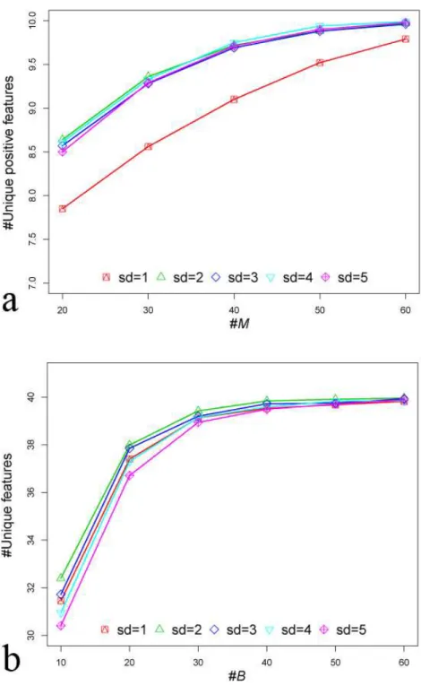
For synthetic datasetS1,Mwas set to be 50, because we observed that whenMwas set to 50, enough or all unique positive features could be obtained from 1,000 features using mRMR (Fig. 4A). Notice that we treated features from the same group as redundant features. After eliminating redundant features, the remaining features wereunique features. If the unique features were from positive marker groups, we called those as
Figure 5 Comparison of results by 4 methods for synthetic datasetS1in selecting non-redundant features.Thex-axis is the standard deviation (sd) representing the parametersds in synthetic dataset
S1. They-axis is the non-redundancy rateEq. (2)in 10 selected features. The error bar represents 95% confidence interval.
groups, we setM′to be 10. In order to determine parameterB, we set a series gradient of the bootstrap process. We observed that whenBwas more than 40, the number of total unique features selected did not increase. Therefore, theBvalue was set to 40 (Fig. 4B). For synthetic datasetS2andS3, we have observed similar patterns (seeSupplemental Information 1for details). Therefore, in this work, parametersM,BandM′were set to be 50, 40 and 10, respectively, for all datasets.
A comparison with current tools using synthetic data
Redundancy analysis based on synthetic datasets
For comparison of 4 methods as regard to redundancy rate (Eq. (1)), non-redundancy rate (Eq. (2)) and error rate (Eq. (3)), we applied LEfSe, Metastats, a bottom-up method Wilcoxon rank-sum test (Wilcoxon) and our method (MetaBoot) on synthetic datasetS1 (There are 10 positive biomarker groups and each group has 10 redundant biomarkers.), respectively. As shown inFig. 5, MetaBoot can select more non-redundant positive features than LEfSe, Metastats and Wilcoxon. Additionally, because the 100 positive markers have the samep-value (see “Materials and Methods” for details), Metastats inFig. 5does not include error bars which indicate that the 10 selected features are from the same positive marker group (the first positive maker group). Therefore, Metastats could not eliminate redundant features when analyzing synthetic datasetS1.
Table 3 Results about redundancies when applied these methods on synthetic datasetS2(Mixture dataset) andS3(Gamma dataset) to select 10 features.In columns for “LEfSe,” “Metastats,” “Wilcoxon” and “MetaBoot,” the values were the non-redundancy rate (Eq. (2)) of non-redundant biomarkers with standard deviation of 1.
Dataset LEfSe Metastats Wilcoxon MetaBoot
S2(Mixture dataset) 36.0±5.5 26.0±5.5 38.0±8.4 42.0±4.5
S3(Gamma dataset) 46.0±11.4 31.4±9.0 50.0±12.2 50.9±8.1
Table 4 Results about robustness when applied these methods on synthetic dataset S2(Mixture dataset) andS3(Gamma dataset) to select 100 positive features.In columns for “LEfSe,” “Metastats,” “Wilcoxon” and “MetaBoot,” the values were “# of positive features” with standard deviation of 1.
Dataset LEfSe Metastats Wilcoxon MetaBoot
S2(Mixture dataset) 67.2±2.6 48.6±4.0 69.0±2.5 70.1±1.1
S3(Gamma dataset) 70.4±5.5 73.3±2.9 83.4±2.3 81.6±2.8
synthetic datasetS3(Table 3), LEfSe and Metastats could only select less than 5 out of 10 non-redundant positive features on average. Both Wilcoxon and MetaBoot outperformed LEfSe and Metastats in that they both can select at least 5 out of 10 non-redundant positive biomarkers. Among these two, MetaBoot was slightly better than Wilcoxon in selecting non-redundant positive markers.
When we further analyzed the differences between MetaBoot and mRMR, we could observe that MetaBoot had similar ability with mRMR in selecting unique positive markers based on synthetic datasetS1(seeFig. S2for details),S2(non-redundancy rate: 48.0%±11.0) andS3(non-redundancy rate: 53.6%±10.1). However, for most synthetic datasets fromS1,S2andS3, mRMR usually had about 10% error rate (Eq. (3)), while MetaBoot had much lower error rate (details of results not shown here).
Robustness analysis based on synthetic datasets
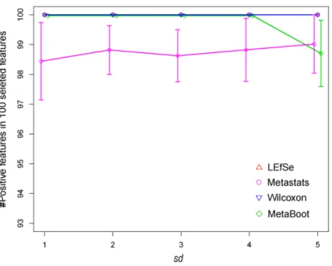
We have applied LEfSe, Metastats, Wilcoxon and MetaBoot on synthetic datasetS1,S2and S3to study their robustness defined by their ability to differentiate positive and negative biomarkers, respectively. For each method, 100 features (equal to the number of redundant positive markers in synthetic datasets) were selected as biomarkers; then, the correctly detected biomarkers were counted. Results (Table 4andFig. 6) have shown that MetaBoot and Wilcoxon method can detect larger number of correct biomarkers compared to other methods. Although all four methods were shown to be robust on synthetic datasetS1 (based on normal distribution), Wilcoxon and MetaBoot outperformed Metastats and LEfSe greatly on synthetic datasetS2(based on the mixture of normal and gamma distribution) andS3(based on gamma distribution), indicating the superiority of Wilcoxon and MetaBoot methods as regard to robustness.
Figure 6 Comparison of results by 4 methods for synthetic dataset S1 in selecting positive fea-tures.Thex-axis is the standard deviation (sd) representing the parametersds in synthetic datasetS1. They-axis is the number of positive features in 100 selected features. The error bar represents standard deviation of 1.
67.4±3.6) andS3(#positive features: 80.2±3.0). The built-in bootstrap process in
MetaBoot might attribute to MetaBoot’s advantage in selecting more positive biomarkers compared to mRMR.
Classification accuracy analysis based on synthetic datasets
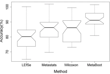
For comparison of different methods in classification accuracy (Eq. (4)), we have applied LEfSe, Metastats, Wilcoxon and MetaBoot on synthetic datasetS3to select 10 features by each of the methods. We then used these 10 features to perform classification by utilizing Support Vector Machine (SVM) implemented by LIBSVM (Chang & Lin, 2011). The reason that we have not done classification based on synthetic datasetS1was the large difference between 2 classes, making classification easy-proof by all methods.
Each class has 60 samples in synthetic datasetS3. We have performed 6-fold cross-validation to estimate the classification accuracy. Therefore, in the aforementioned formula, the average classification accuracy is shown inFig. 7. The highest accuracy was obtained when using 10 features selected by MetaBoot. We also observed that MetaBoot had the most stable classification performance (Fig. 7). We obtained similar results for synthetic datasetS2(seeFig. S3for details).
Biomarker identification based on real metagenomic datasets
Results on oral dataset1
Figure 7 Comparison of accuracies when using 10 features selected by 4 methods based on synthetic datasetS3.Thex-axis represents 4 methods andy-axis represents classification accuracy by SVM.
“Materials and Methods”). We have applied the same four methods on oral dataset1 to select 10 features. Biomarker identification results were shown inFig. 8.
FromFig. 8A, we observed that MetaBoot selected similar features (9 overlaps) with Wilcoxon, while only 4 and 5 feature overlapping with MetaBoot were found for LEfSe and Metastats, respectively. As shown inFig. 8B, the 10 features selected by each of these methods could be assigned to 6–7 phyla which are mostly overlapping. As shown inFig. 8, we observed thatStreptococcuswere selected by MetaBoot, as well as LEfSe and Metastats. Streptococcuswas linked with all kinds of oral problems (Munro & Grap, 2004;Fitzgerald, 1960;Jenkinson & Lamont, 2005). Therefore,Streptococcuscan serve as biomarker to distinguish different samples and be used for oral diagnosis (Bisno et al., 1997).Rothiawere selected by Wilcoxon, as well as LEfSe.Rothiais part of the normal community of microbes residing in the mouth. Previous work foundRothiain 3% of isolates of nitrate-reducing bacteria from the mouth (Doel et al., 2005).
To compare the discriminations accuracy of 10 features selected by different methods, we performed classification by LIBSVM (Chang & Lin, 2011). Each class in oral dataset1 has 50 samples. And we did 5-fold cross-validation (40 samples are used as training datasets) to estimate the classification accuracy. The classification results were shown in
Fig. 9, from which we could observe that MetaBoot still had the highest accuracy and the most stable classification performance.
Figure 8 (...continued)
tree of oral dataset1 at genus level. The tree was generated with RAxML and viewed in ITOL (Letunic & Bork, 2007). Genera are color-coded by phyla, except for the Firmicutes and Proteobacteria, which are shown at class level. We used the same phylogenetic tree plot from microbiome.osu.edu (Griffen et al., 2011), and we added legends onto this tree to show biomarkers selected by different methods.
Figure 9 Comparison of accuracies when using 10 features selected by 4 methods based on oral dataset1.Thex-axis represents 4 methods and they-axis represents the classification accuracy by SVM.
can be attributed to the bootstrap process included in MetaBoot. Therefore, apart from advantage in robustness, biomarkers selected by MetaBoot were considered more biologically meaningful comparing to mRMR (seeFig. S4for details).
Results on oral dataset2
2000), andTreponemawas reported to be associated with periodontal diseases (Chan & McLaughlin, 2000;Sela, 2001). But forPropionibacteriaceae(Fig. 10B), which was selected by LEfSe and Wilcoxon, though this species could be isolated from normal, gingivitis and periodontitis sample with small amount (Riggio et al., 2011), there was few report about the relationship between oral disease andPropionibacteriaceae. Therefore, these results on real oral samples have clearly shown the advantage of MetaBoot on discovery of biologically meaningful biomarkers.
Results on soil samples
For this dataset, we aim to identify biomarkers that could differentiate “pH=4.9” and “pH=8.4” from 16S rRNA sequencing data (details in “Materials and Methods”). Unlike two previous oral datasets that we have used in “Results on oral dataset1” and “Results on oral dataset2,” each class in soil dataset only has 7 samples. Therefore, we focused on the different features selected by different methods not the distribution properties of features. (The sample size is small for distribution analysis). Due to the complexity of soil microbial community samples, we chose taxa at phylum level for analysis.
When we performed classification by LIBSVM (Chang & Lin, 2011), the classification accuracy was always 100% regardless of either of the 5 or 10 features (selected by the four different methods) we used. For soil dataset, features selected by the four different methods all had distinguishing ability to identify different samples. However, biological explanation of features selected by the four different methods needed further research.
Based on the above results for soil samples, we could observe that features selected by the four different methods were quite different (Fig. 11A), yet most of these features had distinguishing power to identify different samples. Further investigation and interpretation of these features might provide more biological insights for the underline functionality of microbial community.
As shown inFig. 11B,Burkholderiaceae(selected by the four methods) was enriched in acidic condition (pH=4.9). But when pH of soil was 8.5, its relative abundance was low. And from different pH samples, the relative abundance ofBurkholderiaceaehad a significant difference (p-value=0.00058). Therefore,Burkholderiaceaecould serve as marker to differentiate soil samples with different pH values. Previous work has reported thatBurkholderiaceaeneeds oxalic acid as its source of carbon (Garrity, Bell & Lilburn, 2004), which partially support this finding.
CONCLUSIONS
The research in metagenomics becomes more and more popular as microbial communities were found to play important roles in many areas such as bioenergy, bioremediation and human health. The discovery of biomarker taxa for metagenomic datasets could facilitate identification of microbial community’s phenotype, thus making them important for community identification and even monitoring of the host or environment within which the community live.
Figure 11 Biomarker identification results on soil dataset.(A) The Venn diagram when we selected top 10 features from soil dataset using the four methods. (B) The bar-chart of average relative abundance of 5 features selected by MetaBoot under different pH values. The values for “Others” are computed as the average for other taxa. The dataset is small for standard parametric approaches. Therefore, thep-values (*, 0.01≤p-value<0.05; **,p-value<0.01) were calculated through permutation tests (a one-way exact test) (Kabacof, 2011). For these five features selected, the exact test indicates a significant difference (p-values are all less than 0.01) between two different pH samples.
We have proposed the MetaBoot method for metagenomic biomarker identification, which is a top-down method based on mRMR strategy and bootstrapping technique. The use of mRMR could reduce redundancies, while the use of bootstrapping could improve robustness of the MetaBoot method. It has been compared with two top-down methods (Metastats and LEfSe) and one bottom-up method (Wilcoxon rank-sum test) on simulated datasets, with results indicating that MetaBoot could identify more non-redundant biomarkers with high accuracy and robustness. On real oral and soil metagenomic datasets, it was also observed that MetaBoot could identify more reliable biomarkers for distinguish different types of microbial communities, showing that the results of MetaBoot were more biologically meaningful. Therefore, MetaBoot could serve well for metagenomic biomarker discovery.
Current taxonomical biomarker discovery methods still face several obstacles: Firstly most of them could identify biomarkers from only two groups of microbial communities, while biomarkers for a set of different groups could be more useful in several circum-stances. Secondly, the biomarker sets (with multiple biomarkers) might be useful for complex samples such as microbial community, yet none has been done on how such sets could be optimized. Thirdly, with the advancement of whole genome sequencing, important functional biomarker identification using not only taxa but also genes would become feasible as well, yet current methods cannot identify functional biomarkers well. All these analytical bottlenecks will be addressed in the future development of MetaBoot and companion tools, and they in turn will help for better understanding of microbial communities and their impacts on our environment.
ACKNOWLEDGEMENTS
We thank Dr. Shi Huang for discussions about building MetaBoot, and Xingzhi Chang for comments about writing codes.
ADDITIONAL INFORMATION AND DECLARATIONS
Funding
This work was supported by the Chinese Academy of Sciences’ e-Science grant INFO-115-D01-Z006, Ministry of Science and Technology’s high-tech (863) grant 2012AA02A707 and 2014AA21502, NSFC grant 61103167, and NSFC grant 31072115. The funders had no role in study design, data collection and analysis, decision to publish, or preparation of the manuscript.
Grant Disclosures
The following grant information was disclosed by the authors: Chinese Academy of Sciences e-Science: INFO-115-D01-Z006.
Competing Interests
All authors declare there are no competing interests.
Author Contributions
• Xiaojun Wang conceived and designed the experiments, performed the experiments, analyzed the data, contributed reagents/materials/analysis tools, wrote the paper, prepared figures and/or tables, reviewed drafts of the paper.
• Xiaoquan Su and Xinping Cui contributed reagents/materials/analysis tools, reviewed drafts of the paper.
• Kang Ning conceived and designed the experiments, performed the experiments, analyzed the data, contributed reagents/materials/analysis tools, wrote the paper, reviewed drafts of the paper.
Supplemental Information
Supplemental information for this article can be found online athttp://dx.doi.org/ 10.7717/peerj.993#supplemental-information.
REFERENCES
Bauer DF. 1972.Constructing confidence sets using rank statistics.Journal of the American Statistical Association67:687–690DOI 10.1080/01621459.1972.10481279.
Birnbaum Z, Tingey FH. 1951.One-sided confidence contours for probability distribution functions.The Annals of Mathematical Statistics22:592–596DOI 10.1214/aoms/1177729550.
Bisno AL, Gerber MA, Kaplan EL, Schwartz RH. 1997.Diagnosis and management of group A streptococcal pharyngitis: a practice guideline.Clinical Infectious Diseases25:574–583 DOI 10.1086/513768.
Caporaso JG, Lauber CL, Walters WA, Berg-Lyons D, Lozupone CA, Turnbaugh PJ, Fierer N, Knight R. 2011.Global patterns of 16S rRNA diversity at a depth of millions of sequences per sample.Proceedings of the National Academy of Sciences of the United States of America
108:4516–4522DOI 10.1073/pnas.1000080107.
Chan E, McLaughlin R. 2000.Taxonomy and virulence of oral spirochetes.Oral Microbiology and Immunology15:1–9DOI 10.1034/j.1399-302x.2000.150101.x.
Chang CC, Lin CJ. 2011.LIBSVM: a library for support vector machines.ACM Transactions on Intelligent Systems and Technology2(3):27DOI 10.1145/1961189.1961199.
DeSantis TZ, Hugenholtz P, Larsen N, Rojas M, Brodie EL, Keller K, Huber T, Dalevi D, Hu P, Andersen GL. 2006.Greengenes, a chimera-checked 16S rRNA gene database and workbench compatible with ARB.Applied and Environmental Microbiology72:5069–5072 DOI 10.1128/AEM.03006-05.
Ding C, Peng H. 2003.Minimum redundancy feature selection from microarray gene expression data.IEEE523–528.
Ding C, Peng H. 2005.Minimum redundancy feature selection from microarray gene expression data.Journal of Bioinformatics and Computational Biology3:185–205
DOI 10.1142/S0219720005001004.
Doel JJ, Benjamin N, Hector MP, Rogers M, Allaker RP. 2005.Evaluation of bacterial nitrate reduction in the human oral cavity.European Journal of Oral Sciences113:14–19
Downes J, Wade WG. 2006.Peptostreptococcus stomatissp. nov., isolated from the human oral cavity.International Journal of Systematic and Evolutionary Microbiology56:751–754 DOI 10.1099/ijs.0.64041-0.
Eisen JA. 2007.Environmental shotgun sequencing: its potential and challenges for studying the hidden world of microbes.PLoS Biology5:e82DOI 10.1371/journal.pbio.0050082.
Fitzgerald RJ. 1960.Demonstration of the etiologic role of streptococci in experimental caries in the hamster.Journal of the American Dental Association61:9–13
DOI 10.14219/jada.archive.1960.0138.
Garrity GM, Bell JA, Lilburn TG. 2004.Taxonomic outline of the prokaryotes. In:Bergey’s manual of systematic bacteriology. Berlin, Heidelberg: Springer.
Goll J, Rusch DB, Tanenbaum DM, Thiagarajan M, Li K, Meth´e BA, Yooseph S. 2010.
METAREP: JCVI metagenomics reports—an open source tool for high-performance
comparative metagenomics.Bioinformatics26:2631–2632DOI 10.1093/bioinformatics/btq455.
Golub TR, Slonim DK, Tamayo P, Huard C, Gaasenbeek M, Mesirov JP, Coller H, Loh ML, Downing JR, Caligiuri MA. 1999.Molecular classification of cancer: class discovery and class prediction by gene expression monitoring.Science286:531–537
DOI 10.1126/science.286.5439.531.
Gower JC. 1966.Some distance properties of latent root and vector methods used in multivariate analysis.Biometrika53:325–338DOI 10.1093/biomet/53.3-4.325.
Griffen AL, Beall CJ, Firestone ND, Gross EL, DiFranco JM, Hardman JH, Vriesendorp B, Faust RA, Janies DA, Leys EJ. 2011.CORE: a phylogenetically-curated 16S rDNA database of the core oral microbiome.PLoS ONE6:e19051DOI 10.1371/journal.pone.0019051.
Han XY, Falsen E. 2005.Characterization of oral strains of Cardiobacterium valvarum and emended description of the organism.Journal of Clinical Microbiology 43:2370–2374 DOI 10.1128/JCM.43.5.2370-2374.2005.
Huang S, Li R, Zeng X, He T, Zhao H, Chang A, Bo C, Chen J, Yang F, Knight R. 2014.Predictive modeling of gingivitis severity and susceptibility via oral microbiota.The ISME Journal
8:1768–1780DOI 10.1038/ismej.2014.32.
Huson DH, Auch AF, Qi J, Schuster SC. 2007.MEGAN analysis of metagenomic data.Genome Research17:377–386DOI 10.1101/gr.5969107.
Jenkinson HF, Lamont RJ. 2005.Oral microbial communities in sickness and in health.Trends in Microbiology13:589–595DOI 10.1016/j.tim.2005.09.006.
Jurkowski A, Reid AH, Labov JB. 2007.Metagenomics: a call for bringing a new science into the classroom (while it’s still new).CBE-Life Sciences Education6(4):260–265
DOI 10.1187/cbe.07-09-0075.
Kabacof R. 2011.R in action. Shelter Island: Manning Publications Co.
Kristiansson E, Hugenholtz P, Dalevi D. 2009.ShotgunFunctionalizeR: an R-package for functional comparison of metagenomes.Bioinformatics25:2737–2738
DOI 10.1093/bioinformatics/btp508.
Lam PK, Gray JS. 2003.The use of biomarkers in environmental monitoring programmes.Marine Pollution Bulletin46:182–186DOI 10.1016/S0025-326X(02)00449-6.
Letunic I, Bork P. 2007.Interactive Tree Of Life (iTOL): an online tool for phylogenetic tree display and annotation.Bioinformatics23:127–128DOI 10.1093/bioinformatics/btl529.
Lozupone C, Knight R. 2005.UniFrac: a new phylogenetic method for comparing microbial communities.Applied and Environmental Microbiology71:8228–8235
DOI 10.1128/AEM.71.12.8228-8235.2005.
Meyer F, Paarmann D, D’souza M, Olson R, Glass E, Kubal M, Paczian T, Rodriguez A, Stevens R, Wilke A. 2008.The metagenomics RAST server—a public resource for the automatic phylogenetic and functional analysis of metagenomes.BMC Bioinformatics
9:386DOI 10.1186/1471-2105-9-386.
Munro CL, Grap MJ. 2004.Oral health and care in the intensive care unit: state of the science. American Journal of Critical Care13(1):25–34.
Parks DH, Beiko RG. 2010.Identifying biologically relevant differences between metagenomic communities.Bioinformatics26:715–721DOI 10.1093/bioinformatics/btq041.
Pedr ´os-Ali ´o C. 2006.Marine microbial diversity: can it be determined?Trends in Microbiology
14:257–263DOI 10.1016/j.tim.2006.04.007.
Proctor GN. 1994.Mathematics of microbial plasmid instability and subsequent differential growth of plasmid-free and plasmid-containing cells, relevant to the analysis of experimental colony number data.Plasmid32:101–130DOI 10.1006/plas.1994.1051.
Riggio MP, Lennon A. 2003.Identification of oral Peptostreptococcus isolates by PCR-restriction fragment length polymorphism analysis of 16S rRNA genes.Journal of Clinical Microbiology
41:4475–4479DOI 10.1128/JCM.41.9.4475-4479.2003.
Riggio MP, Lennon A, Taylor DJ, Bennett D. 2011.Molecular identification of bacteria associated with canine periodontal disease.Veterinary Microbiology150:394–400
DOI 10.1016/j.vetmic.2011.03.001.
Schloss PD, Handelsman J. 2005.Introducing DOTUR, a computer program for defining operational taxonomic units and estimating species richness.Applied and Environmental Microbiology71:1501–1506DOI 10.1128/AEM.71.3.1501-1506.2005.
Schloss PD, Handelsman J. 2006a.Introducing SONS, a tool for operational taxonomic unit-based comparisons of microbial community memberships and structures.Applied and Environmental Microbiology72:6773–6779DOI 10.1128/AEM.00474-06.
Schloss PD, Handelsman J. 2006b.Introducing TreeClimber, a test to compare microbial community structures. Applied and Environmental Microbiology 72:2379–2384 DOI 10.1128/AEM.72.4.2379-2384.2006.
Schloss PD, Westcott SL, Ryabin T, Hall JR, Hartmann M, Hollister EB, Lesniewski RA, Oakley BB, Parks DH, Robinson CJ. 2009. Introducing mothur: open-source, platform-independent, community-supported software for describing and comparing microbial communities. Applied and Environmental Microbiology 75:7537–7541 DOI 10.1128/AEM.01541-09.
Segata N, Izard J, Waldron L, Gevers D, Miropolsky L, Garrett WS, Huttenhower C. 2011.
Metagenomic biomarker discovery and explanation.Genome Biology12:R60 DOI 10.1186/gb-2011-12-6-r60.
Sela MN. 2001.Role of Treponema denticola in periodontal diseases.Critical Reviews in Oral Biology & Medicine12:399–413DOI 10.1177/10454411010120050301.
Shapiro SS, Wilk MB. 1965.An analysis of variance test for normality (complete samples). Biometrika52:591–611DOI 10.1093/biomet/52.3-4.591.
Slotnick I, Dougherty M. 1964.Further characterization of an unclassified group of bacteria causing endocarditis in man:Cardiobacterium hominisgen. et sp. n.Antonie van Leeuwenhoek
Su XQ, Pan WH, Song BX, Xu J, Ning K. 2014.Parallel-META 2.0: enhanced metagenomic data analysis with functional annotation, high performance computing and advanced visualization. PLoS ONE9(3):e89323DOI 10.1371/journal.pone.0089323.
Su X, Xu J, Ning K. 2012.Meta-Storms: efficient search for similar microbial communities based on a novel indexing scheme and similarity score for metagenomic data.Bioinformatics
28:2493–2501DOI 10.1093/bioinformatics/bts470.
Swan KA, Curtis DE, McKusick KB, Voinov AV, Mapa FA, Cancilla MR. 2002.High-throughput gene mapping in Caenorhabditis elegans.Genome Research12(7):1100–1105.
Tothill RW, Tinker AV, George J, Brown R, Fox SB, Lade S, Johnson DS, Trivett MK, Etemadmoghadam D, Locandro B. 2008.Novel molecular subtypes of serous and
endometrioid ovarian cancer linked to clinical outcome.Clinical Cancer Research14:5198–5208 DOI 10.1158/1078-0432.CCR-08-0196.
White JR, Nagarajan N, Pop M. 2009.Statistical methods for detecting differentially abundant features in clinical metagenomic samples.PLoS Computational Biology5(4):e1000352 DOI 10.1371/journal.pcbi.1000352.