Claudinei de Moura Altea
Computational Determination of Convective
Heat Transfer and Pressure Drop
Coefficients of Hydrogenerators Ventilation
System
Dissertation presented to Escola Politécnica
da Universidade de São Paulo for the partial
requirement for the degree of Master of
Science in Mechanical Engineering
Supervisor: Prof. Dr. Jurandir Itizo Yanagihara
Este exemplar foi revisado e corrigido em relação à versão original, sob responsabilidade única do autor e com a anuência de seu orientador.
São Paulo, ______ de ____________________ de __________
Assinatura do autor: ________________________
Assinatura do orientador: ________________________
Catalogação-na-publicação
Altea, Claudinei de Moura
Computational determination of convective heat transfer and pressure drop coefficients of hydrogenerators ventilation system / C. M. Altea -- versão corr. -- São Paulo, 2016.
154 p.
Dissertação (Mestrado) - Escola Politécnica da Universidade de São Paulo. Departamento de Engenharia Mecânica.
Dedicatory
Acknowledgments
Above all, I thank God for having blessed me with a wonderful family, great opportunities and the provision of all my needs to walk his proposed ways for me, including the accomplishment of this work.
To my supervisor, Prof. Dr. Jurandir Itizo Yanagihara, for the thrust and belief from the earliest and all the support along the whole work.
To the company Voith Hydro and all the friends I have by been working there. For the knowledge acquired working for years with engineering teams, their support and encouragement for this work, as well the support from the workshop, field service and commissioning (HPP Teles Pires) colleagues for their support with field measurements development.
Resumo
O objetivo do presente trabalho é determinar os coeficientes de perda de carga e transferência de calor, normalmente aplicados nos cálculos analíticos de design térmico de hidrogeradores, obtido pela aplicação de cálculo numérico (Computacional Fluid Dynamics - CFD) e validado por resultados experimentais e medições de campo. O objeto de estudo é limitado à região mais importante do sistema de ventilação (os dutos de ar de arrefecimento do núcleo do estator) para obter resultados numéricos dos coeficientes de transferência de calor e de perda de carga, que são impactados principalmente pela entrada de dutos de ar.
Os cálculos numéricos consideraram escoamentos tridimensionais, em regime permanente, incompressíveis e turbulentos; e foram baseados no método dos volumes finitos. Os cálculos de escoamento turbulento foram realizados com procedimentos baseados em equações médias (RANS), utilizando o modelo k-omega SST (Shear-Stress Transport) como modelo de turbulência. Métricas de qualidade de malha foram monitoradas e as incertezas devido à erros de discretização foram avaliadas por meio de um estudo de independência de malha e aplicação de um procedimento de estimativa de incertezas com base na extrapolação de Richardson.
Finalmente, uma série de cálculos numéricos, variando parâmetros geométricos do design da entrada do duto de ar e dados operacionais, foram executados a fim de se obter curvas de tendência para coeficientes de perda de carga (resultados deste trabalho) a serem aplicadas diretamente à rotinas de cálculos analíticos de sistemas completos de ventilação de hidrogeradores. Paralelamente à isso, o cálculo térmico numérico foi executado na simulação do protótipo, a fim de se definir o coeficiente de transferência de calor por convecção.
Abstract
The objective of the present work is to determinate the pressure drop and the heat transfer coefficients, normally applied to analytical calculations of hydrogenerators thermal design, obtained by applying numerical calculation (Computational Fluid Dynamics – CFD) and validated by experimental results and field measurements. The object of study is limited to the most important region of the ventilation system (the cooling air ducts of stator core) to get numerical results of heat transfer and pressure drop coefficients, which are impacted mostly by the entrance of air ducts.
The numerical calculations considered three-dimensional, steady-state, incompressible and turbulent flow; and were based on the Finite Volume methodology. The turbulent flow computations were carried out with procedures based on RANS equations by selecting k-omega SST (Shear-Stress Transport) as turbulence model. Grid quality metrics were monitored and the uncertainties due to discretization errors were evaluated by means of a grid independence study and application of an uncertainty estimation procedure based on Richardson extrapolation.
The validation of numerical method developed by the present work (specifically to simulate the flow dynamics behavior and to obtain numerically the pressure drop coefficient of the airflow to enter and pass through the Stator Core Air Duct in a hydrogenerator) is performed by comparing the numerical results to experimental data published by Wustmann (2005). The reference experimental data were obtained by a model test. The comparison between numerical and experimental results shows that the difference of pressure drop for Reynolds numbers higher than 5000 is 2% at maximum, while for lower Reynolds numbers, the difference increases significantly and reaches 10%. It is presented that the most reasonable hypothesis for higher discrepancy at lower Reynolds numbers can be assigned to the experiment’s non-steady-state condition. It is to conclude that the proposed numerical method is validated for the upper region of the analyzed range. Additionally to the model test validation, field measurements were executed in order to confirm numerical results. Measurements of pressure drop in the stator core of a real hydrogenerator were a challenge. Nevertheless, despite all the difficulties and considerable high field measuring uncertainties, trend curves behavior are similar to numerical results.
ventilation systems. Parallel to it, thermal numerical calculation was executed in the prototype simulation in order to define the convective heat transfer coefficient.
VIII
Table of Contents
List of Figures ... 11
List of Tables ... 16
List of Symbols ... 17
List of Abbreviations and Acronyms ... 20
1 Introduction ... 21
1.1 Hydrogenerators ... 21
1.1.1 Hydrogenerators Cooling System ... 22
1.1.2 Hydrogenerators Ventilation Systems ... 23
1.1.3 Impact of Ventilation on Hydrogenerators Design ... 24
1.1.4 Verifications of Ventilation System ... 25
1.1.5 Model Tests ... 28
1.1.6 Field Measurements ... 29
1.1.7 Numerical Calculation ... 29
1.2 Objective ... 30
1.3 Object of Study ... 30
2 Literature Review ... 33
2.1 Experimental Analysis ... 33
2.2 Numerical Analysis and Experimental Validation ... 35
3 Computational Procedure ... 41
3.1 Solution Strategy ... 41
3.2 The Numerical Method ... 41
3.2.1 Governing Equations ... 42
3.2.2 The Finite Volume Method ... 43
3.2.3 Spatial Discretization Scheme ... 46
3.2.3.1 Taylor Series Expansion... 47
3.2.3.2 Upwind Interpolation (UDS) ... 48
3.2.3.3 High Resolution Scheme... 50
3.2.4 Shape Functions ... 50
3.2.5 Pressure-Velocity Coupling ... 52
3.2.6 Solution of Linear Equation Systems ... 54
3.2.7 Turbulence ... 56
3.2.7.1 Reynolds-Averaged Navier–Stokes (RANS) Equations ... 57
3.2.7.2 The − Model ... 61
IX
3.2.7.4 The SST − Model ... 63
3.2.7.5 Near-Wall Treatments ... 64
3.2.7.6 Summary of Turbulence Models ... 65
3.2.8 Discretization Grid ... 68
3.2.8.1 Grid Quality ... 69
3.2.8.2 Grid Quality Metrics ... 69
3.2.8.3 Grid Quality Metrics – Aspect ratio ... 70
3.2.8.4 Grid Quality Metrics – Orthogonality and Skewness ... 70
3.2.8.5 Grid Quality Metrics – Others Individual Cell Metrics ... 72
3.2.8.6 Grid Quality Metrics – Metrics for Domain Regions ... 72
4 Reference Laboratory and Field Measurements Data ... 74
4.1 Reference Laboratory Experimental Data from the Literature ... 74
4.2 Reference Field Measurement Data of Prototype ... 80
4.2.1 Development of Measurement Procedures and Devices ... 80
4.2.2 Installation of Measurement Devices at Site ... 81
4.2.3 Field Measurements ... 85
4.2.3.1 Measurement Instruments and Devices Arrangement ... 87
4.2.3.2 Field Measurements Uncertainty Analysis ... 89
4.2.3.2.1 Uncertainties of Evaluation Type A ... 89
4.2.3.2.2 Uncertainties of Evaluation Type B ... 90
4.2.3.2.3 Uncertainties Combination ... 91
4.2.3.3 Field Measurements Results ... 93
5 Application to the Model Test and Prototype Geometries and Conditions ... 96
5.1 Numerical Calculation Applied to the Model Test ... 96
5.1.1 Computational Domain... 96
5.1.2 Boundary Conditions ... 98
5.1.3 Discretization Grid ... 99
5.1.3.1 Verification of Grid Quality Metrics ... 101
5.1.3.2 Grid Independence Study ... 103
5.1.3.3 Estimation of Uncertainty due to Discretization Errors ... 104
5.2 Numerical Calculation Applied to the Prototype ... 106
5.2.1 Computational Domain... 106
5.2.2 Boundary Conditions ... 111
5.2.3 Discretization Grid ... 112
X
6 Results ... 116
6.1 Numerical Method Validation by Model Test ... 116
6.1.1 Flow Field Results ... 116
6.1.2 Experimental and Numerical Data Comparisons ... 118
6.2 Numerical Results Applied to the Prototype... 121
6.2.1 Flow Field Results ... 121
6.2.2 Field Measurements and Numerical Data Comparison ... 125
6.3 Determination of Coefficients ... 126
6.3.1 Pressure Drop Coefficient ... 127
6.3.2 Convective Heat Transfer Coefficient ... 136
7 Conclusions ... 142
7.1 Scope for Future Work ... 144
References ... 145
Appendix ... 150
Appendix A: Uncertainty of Pressure Measurements ... 150
Appendix B: Uncertainty of Velocity Measurements... 151
Appendix C: Numerical Results of Pressure Standard Uncertainties ... 152
Appendix D: Numerical Results of Velocity Standard Uncertainties ... 153
XI
List of Figures
Figure 1.1 - Example of hydrogenerator – Sanxia (Kramer, Haluska Jr., & Namoras, 2001). 21
Figure 1.2 - Axial-Radial ventilation systems (Meyer, 2006). ... 23
Figure 1.3 - Radial-Radial ventilation system (Meyer, 2006). ... 24
Figure 1.4 - Fluid Dynamics Network model of ventilation system (Meyer, 2006). ... 26
Figure 1.5 - Example of fluid dynamics calculation result (Meyer, 2006). ... 27
Figure 1.6 - Application of calculation methods (Ujiie, Arlitt, & Etoh, 2006). ... 30
Figure 1.7 - Typical stator core including stator winding bar. ... 31
Figure 1.8 - Costs of hydrogenerator components (Kramer, Haluska Jr., & Namoras, 2001). 32 Figure 2.1 - Comparison of pressure drop coefficients – experimental and numerical results (Wustmann, 2005). ... 34
Figure 2.2 - PIV measurements on stator core air ducts (Hartono, Golubev, Moradnia, Chernoray, & Nilsson, 2012a). ... 35
Figure 2.3 - Design proposed by Yanagihara & Rodrigues (1998). ... 36
Figure 2.4 - Velocity profile measurements on stator core air ducts outlet (Moradnia, Chernoray, & Nilsson, 2012a). ... 39
Figure 3.1 - Typical control volume definition (ANSYS CFX, 2012). ... 44
Figure 3.2 - Typical grid element (ANSYS CFX, 2012). ... 45
Figure 3.3 - Typical control volume and notation for Cartesian 2D grid (Ferziger & Peric, 2002). ... 48
Figure 3.4 – Left: Discritized solution. Right: Semeared solution (numerical diffusion) by first order UDS. (ANSYS CFX, 2012). ... 49
Figure 3.5 – Left: Discritized solution. Right: Numeical oscilation by second order UDS. (ANSYS CFX, 2012). ... 50
Figure 3.6 – Hexahedral Element. (ANSYS CFX, 2012). ... 51
Figure 3.7 - 1D grid example of co-located arrangement (Versteeg & Malalasekera, 2007). .. 52
Figure 3.8 - 1D grid example of staggered arrangement (Versteeg & Malalasekera, 2007). . 54
Figure 3.9 – Behaviour of Algebraic Multigrid method (ANSYS CFX, 2012). ... 56
XII
Figure 3.11 – Subdivisions of the Near-Wall Region (ANSYS CFX, 2012). ... 64
Figure 3.12 - Skewnness on a hexaedrical cell (ANSYS ICEM, Inc., 2012) ... 71
Figure 3.13 - Improvement of orthogonality (Ferziger & Peric, Computational Methods for Fluid Dynamics, 2002). ... 71
Figure 3.14 - Left: warping on hexaedrical cell (Ferziger & Peric, 2002); Right: warping on tetraedrical cell (Tu, Yeoh, & Liu, 2013). ... 72
Figure 3.15 - Dragged vertex on hexaedrical cell. Left: Ferziger & Peric (2002); Right: ANSYS ICEM CFD 14.5 (ANSYS ICEM, Inc., 2012). ... 72
Figure 4.1 – Experiment layout. Based on Wustmann (2005)... 74
Figure 4.2 – Rotor applied on model test (Wustmann, 2005)... 76
Figure 4.3 – Stator applied on model test (Wustmann, 2005). ... 77
Figure 4.4 – Model test wedge applied to the numerical simulation (Wustmann, 2005). ... 77
Figure 4.5 – Experimental complete model (Wustmann, 2005). ... 78
Figure 4.6 – Bypass circuit for flow volume rate measurement (Wustmann, 2005). ... 79
Figure 4.7 – Pressure measurements on model test (Wustmann, 2005). ... 79
Figure 4.8 – Wokshop tests of pressure wall tapping installation. ... 80
Figure 4.9 – Instruction of pressure wall tapping installation at site. ... 81
Figure 4.10 – Scheme of pressure tapping installation. ... 81
Figure 4.11 – Teles Pires UG05 Stator at generator’s pit. ... 82
Figure 4.12 – Stator frame inspection window. ... 83
Figure 4.13 – Axial location of pressure tapping installation. ... 83
Figure 4.14 – Tangential location of pressure tapping installation. ... 84
Figure 4.15 – Example of identified pressure tapping installation. ... 85
Figure 4.16 – Example of field mesasurement execution. ... 86
Figure 4.17 – Delimited areas prepared for measurements of air volume flow passing through one air cooler. ... 87
Figure 4.18 – Mesasurement instruments and devices arrangement. ... 89
Figure 4.19 – Measured results for pressure drop of nine working measuring devices. ... 94
XIII
Figure 4.21 – Measured results for total flow volume rate with uncertainties. ... 95
Figure 5.1 – Computational domain. ... 96
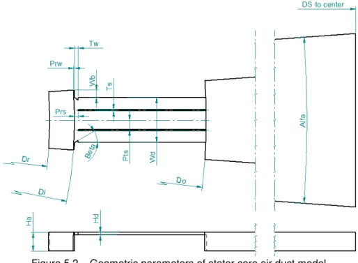
Figure 5.2 – Geometric parameters of stator core air duct model. ... 97
Figure 5.3 – Boundary conditions applied to stator core air duct model. ... 99
Figure 5.4 – Grid applied to the numerical simulations. ... 100
Figure 5.5 – O-Grid blocks applied for boundary layers cells. ... 101
Figure 5.6 – Grid of air duct entrance region (lowest aspect ratio colored). ... 102
Figure 5.7 – Air computational domain of numerical calculation applied to the prototype. ... 106
Figure 5.8 – Detail of axial connection between air ducts in the region of frontal wedges. .. 107
Figure 5.9 – Solid bodies computational domain (assimetric quarter) of numerical calculation applied to the prototype. ... 108
Figure 5.10 – Air volume geometric parameters. ... 109
Figure 5.11 – Boundary conditions applied to the air volume of prototype simulation. ... 112
Figure 5.12 – Grid applied to the prototype numerical simulations. ... 113
Figure 5.13 – O-Grid blocks applied for boundary layers cells. ... 113
Figure 5.14 – Grid of air duct region. ... 115
Figure 6.1 – Grapghic Output – Static pressure. ... 117
Figure 6.2 – Grapghic Output – Volume flow streamlines colored by velocities. ... 117
Figure 6.3 – Comparisons between experimental and numerical results of flow volume rate. ... 118
Figure 6.4 – Comparisons between experimental and numerical results of pressure drop. .. 119
Figure 6.5 – Comparisons between experimental and numerical results of pressure drop coefficient. ... 120
Figure 6.6 – Prototype simulation grapghic output – Static pressure. ... 122
Figure 6.7 – Prototype simulation grapghic output – Streamlines based on core vortex colored by velocity. ... 123
Figure 6.8 – Prototype simulation grapghic output –Volume flow streamlines colored by velocities – Detail. ... 123
Figure 6.9 – Prototype simulation grapghic output – Air temperature. ... 124
XIV Figure 6.11 – Comparisons between field measurements and numerical results of pressure
drop. ... 126
Figure 6.12 – Pressure drop coefficient as function of velocity ratio for 60o frontal wedge without relief. ... 127
Figure 6.13 – Velocity vectors for 60o frontal wedge without relief (Vr/Vt = 0.37). ... 128
Figure 6.14 – Velocity vectors for 60o frontal wedge without relief (Vr/Vt = 1.00). ... 128
Figure 6.15 – Velocity vectors for 60o frontal wedge without relief (Vr/Vt = 1.67). ... 129
Figure 6.16 – Volume flow streamlines colored by velocities for 60o frontal wedge without relief (Vr/Vt = 0.37). ... 130
Figure 6.17 – Volume flow streamlines colored by velocities for 60o frontal wedge without relief (Vr/Vt = 1.00). ... 130
Figure 6.18 – Volume flow streamlines colored by velocities for 60o frontal wedge without relief (Vr/Vt = 1.67). ... 131
Figure 6.19 – Pressure drop coefficient as function of velocity ratio for 60o frontal wedge with 45o relief. ... 132
Figure 6.20 – Velocity vectors for 60o frontal wedge with 45o relief (Vr/Vt = 0.07). ... 133
Figure 6.21 – Velocity vectors for 60o frontal wedge with 45o relief (Vr/Vt = 0.28). ... 133
Figure 6.22 – Velocity vectors for 60o frontal wedge with 45o relief (Vr/Vt = 1.55). ... 134
Figure 6.23 – Volume flow streamlines colored by velocities for 60o frontal wedge with 45o relief (Vr/Vt = 0.07)... 135
Figure 6.24 – Volume flow streamlines colored by velocities for 60o frontal wedge with 45o relief (Vr/Vt = 0.28)... 135
Figure 6.25 – Volume flow streamlines colored by velocities for 60o frontal wedge with 45o relief (Vr/Vt = 1.55)... 136
Figure 6.26 – Convective heat transfer coefficient as function of radial velocity in air channels. ... 137
Figure 6.27 – Temperature of air and solid bodies (Vr = 1.00 m.s-1). ... 138
Figure 6.28 – Temperature of air and solid bodies (Vr = 5.66 m.s-1). ... 138
Figure 6.29 – Temperature of air and solid bodies (Vr = 12.00 m.s-1). ... 139
Figure 6.30 – Temperature of insulation surfaces (Vr = 1.00 m.s-1). ... 140
XVI
List of Tables
Table 1.1 – Hydrogenerators ventilation system according to IEC 34-6 ... 24
Table 3.1 – Classification of turbulence models (Versteeg & Malalasekera, 2007). ... 60
Table 3.2 – Turbulence models applied in the reference works. ... 66
Table 3.3 – Comparisons between − and SST − turbulence models. ... 67
Table 4.1 – Reported constant values for experimental data (Wustmann, 2005) ... 75
Table 4.2 – Slot location of pressure tapping installation ... 84
Table 4.3 – Field measurement instruments and devices for pressure ... 88
Table 4.4 – Others field measurement instruments ... 89
Table 4.5 – Field measurement instruments standard uncertainties ... 90
Table 4.6 – Extra standard uncertainties ... 91
Table 5.1 – Geometric data of numerical calculation... 97
Table 5.2 – Grid quality metrics obtained for validation simulation ... 102
Table 5.3 – Grid quality metrics obtained for validation simulation (only air duct) ... 103
Table 5.4 –Summary of the grid independence study ... 104
Table 5.5 – Estimation of uncertainty due to discretization ... 105
Table 5.6 – Material data of numerical simulation applied to the prototype. ... 108
Table 5.7 – Geometric data of air volume domain. ... 110
Table 5.8 – Grid quality metrics obtained for prototype simulation ... 114
XVII
List of Symbols
English Symbols
acceleration
area
specific heat constant pressure specific heat constant volume
, diameter
duct hydraulic diameter
energy
function
force
acceleration of gravity
ℎ duct width, heat-transfer coefficient by convection, enthalpy electrical current
thermal conductivity characteristic length
mass
mass rate of flow
, amount of elements
, pressure
power index
heat-transfer rate
" heat-transfer rate per unit area
! volume flow rate
" gas constant
# entropy, experimental standard deviation
$ source or sink of scalar quantity
% time
& temperature
', (, ) Cartesian velocity components
* relative air humidity
( specific volume
XVIII
,, -, . Cartesian coordinates
/, 0, 1 generic variables
Dimensionless Groups
Eckert number, V36 ∆&
7 Froude number, V3⁄
Mach number, V⁄
' Nusselt number, 9 ⁄ ∆&
: Peclet number, ": 7
7 Prandtl number, ; ⁄
": Reynolds number, <+ ;⁄
Greek Symbols
= thermal diffusivity
> volumetric thermal expansion coefficient
∆ variation
? specific-heat ratio
@ velocity boundary layer
@∗ displacement boundary layer
@B temperature boundary layer
@C Kronecker delta, @C= 1 if F = G and @C= 0 if F ≠ G
JC strain-rate tensor
K second viscosity coefficient
L similarity variable, efficiency, rotational speed
; dynamic viscosity, standard uncertainties
;M turbulent viscosity
N kinematic viscosity
NM kinematic turbulent or eddy viscosity
O 3.14159…
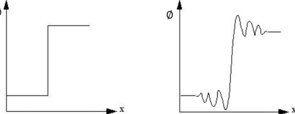
∅ scalar quantity
Q diffusivity of scalar quantity
Q% turbulent or eddy diffusivity
Φ dissipation function
S stream function
XIX
TC stress tensor
vorticity
Ω angular velocity
ζ pressure drop coefficient
Subscripts
∞ far field
0 initial or reference value
cross section
X Y combined
XZ conduction
XZ( convection
7F% critical
: freestream, boundary-layer edge
fluid
:Z generated
F, G, Cartesian coordinates index, counter index
[X## lost
mean
Z normal
7 radiation
) wall
, at position ,
Superscripts
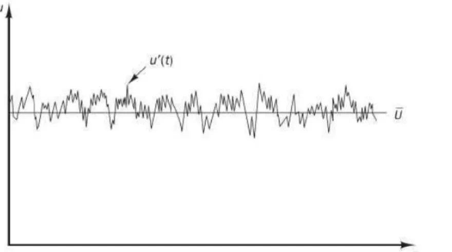
− time mean
′ differentiation
∗ dimensionless variable
XX
List of Abbreviations and Acronyms
AR Aspect Ratio
BDS Backward Difference Scheme CDS Central Difference Scheme CFD Computational Fluid Dynamics CHT Conjugate Heat Transfer
CTA Constant Temperature Anemometry DNS Direct Numerical Simulation
FDS Forward Difference Scheme
HPP Hydro Power Plant
HWA Hot-Wire Anemometry
IEC International Electrotechnical Commission
IC International Code
LDA Laser Doppler Anemometry
LES Large Eddy Simulation
LPTN Lumped Parameter Thermal-Network
MME “Ministério de Minas e Energia” (Ministry of Mines and Energy)
MG Multigrid
MT Mato Grosso (Brazilian State) PA Pará (Brazilian State)
PIV Particle Image Velocimetry
RANS Reynolds-Averaged Navier–Stokes RAM Random Access Memory
SIMPLE Semi-Implicit Method for Pressure-Linked Equations
SST Shear-Stress Transport UDS Upwind Differencing Scheme
UG “Unidade Geradora” (Generation Unit)
VDE “Verband der Elektrotechnik, Elektronik und Informationstechnik” (Association for Electrical, Electronic and Information Technologies)
21
1 Introduction
In 2013, with 88,966 MW of installed capacity, hydropower represents 67% of Brazilian power grid. According to the Brazilian Decennial Plan for Energy Expansion for 2020 (MME, 2011) this value shall be increased to 115,123 MW and will account for 67.3% of power generation.
Considering the growing demand for electricity and the representativeness of the hydroelectricity generation for the country, it is natural that studies of ways to optimize the use of hydraulic resources earn more importance. The study of thermal design of hydrogenerators is included in this context.
1.1 Hydrogenerators
Generator and Moto-generator differ between them according to its functionality (Wiedemann & Kellenberger, 1967). The first one converts mechanical energy into electrical energy and the second one does the same, but also the opposite. When applied in hydroelectric power plants, they are known as Hydrogenerators and Moto-Hydrogenerators. The object of study of this work is the ventilation system of those machines, which will be called just Hydrogenerators from now on.
The components of a hydrogenerator which impact the ventilation design are located both in the stator as in the rotor of the machine, as presented by Kramer, Haluska Jr., & Namoras (2001).
22 1) Rotor Hub: structure made of welded carbon steel which, due to its geometry, contributes in boosting and directing of required air for hydrogenerator cooling.
2) Rotor Rim: structure resulting from stacked and pressed plates of high strength steel which, due to its geometry (creating radial ducts), also contributes in boosting and directing of required air for hydrogenerator cooling, by its rotational movement.
3) Poles: compound of a steel core (stacked and pressed plates) wrapped in copper coil and insulating material. Due to the electric current flowing through the coil, it dissipates heat by Joule effect, which must be removed by the ventilation system. Considering the fact they are salient poles fixed on the rotor (with air occupying the spaces between them), they also contribute in boosting and directing of required air for hydrogenerator cooling.
4) Stator Winding: compound of conductors (bars or coils) of copper and insulating material. Due to the electric current flowing through the conductors, it also loses heat by Joule effect, which must be removed by the ventilation system.
5) Stator Core: structure resulting from stacked and pressed sheets of silicon electrical steel, which is designed to create ducts for the airflow in the radial direction.
6) Stator Frame: structure made of welded carbon steel designed to guide the air from the stator core to the heat exchangers.
7) Heat Exchangers: air-to-water type, responsible for removing heat from the warm air and returning it cooled to the system.
8) Air Guides: carbon steel structure (or fiberglass) responsible for guiding the air in the generator housing and delimiting the boundaries of suction and pressure regions of ventilation system.
Depending on the ventilation system type, components may exist with the sole and exclusive function of boosting the air of the ventilation system: e.g. radial or axial fans (fixed to the hydrogenerator shaft), or motor-fans, which operate independently mounted on stationary structure of the hydrogenerator.
1.1.1 Hydrogenerators Cooling System
23 air circulation system, driven by the hydrogenerator’s shaft (or external motor-fans) is called: "Ventilation System".
There is also the possibility of cooling the hydrogenerator partially with application of pure water as cooling fluid, which flows through internal channels into most critical components: the electrical conductors. However, this kind of cooling system is applied very rarely due to its high costs, and it is not covered by this study.
1.1.2 Hydrogenerators Ventilation Systems
Ventilation systems for medium and large size hydrogenerators can be classified into two groups (Meyer, 2006):
- Axial-Radial Ventilation
- Radial-Radial Ventilation
The names refer to the main direction in which the air is forced to flow in the rotor and the stator, respectively.
In Axial-Radial ventilation systems, the air is introduced into the rotor (space between poles) axially driven by fans, which are fixed to the rotor shaft (radial or axial fans) or work independently (motor-fans), and follows in radial direction through air ducts of stator.
Figure 1.2 - Axial-Radial ventilation systems (Meyer, 2006).
24 Figure 1.3 - Radial-Radial ventilation system (Meyer, 2006).
Wiedemann & Kellenberger (1967) presented a generic classification of cooling systems for electrical machines according to the German standard VDE 0530-6 (1996). Considering the corresponding international standard, IEC 34-6 (1991), the presented ventilation systems above can be classified as shown in Table 1.1.
Table 1.1 – Hydrogenerators ventilation system according to IEC 34-6
Ventilation System IC – According to IEC 34-6
Axial Fan IC8A1W7
Radial Fan IC8A1W7
Motor - Fan IC8A5W7
Rim Ventilation IC8A1W7
1.1.3 Impact of Ventilation on Hydrogenerators Design
Several materials used in the construction of hydrogenerators can withstand only a certain maximum temperature (especially insulating materials) without jeopardizing its properties or affecting its lifetime. Therefore, the detailed study of the ventilation system is essential to prevent damages arising from improper thermal effects.
25 hydrogenerator is designed to last for several decades, the ventilation study becomes relevant for the return of capital employed in a hydroelectric project.
The design of the ventilation system must then ensure that the temperature limits for the respective applied materials are not exceeded, and, at the same time, that the total amount of ventilation losses are minimized in order to maximize the efficiency of the hydrogenerator. An appropriated and adequate ventilation system design is a classic optimization problem, where high precision on calculation procedures is essential.
The complexity of optimization of a ventilation system increases with the size of the hydrogenerator. The electromagnetic losses, which generate heat to be removed by the ventilation system, become greater with the size of the machine.
As a first approximation, it can be asserted that the losses generated in the hydrogenerator ( ^_``) are proportional to its physical size. Keeping certain dimensional proportionality, the machine physical size and hence the generated losses are proportional to its volume, or to the cube of a machine reference dimension.
a ^_``∝ c (1.1)
As the ventilation system works primarily by convection, analogously one can imagine that the external surface and the dissipated heat of this volume are proportional to the square of a machine reference dimension.
d_e ∝ 3 (1.2)
Thus, for large hydrogenerators, the ratio of losses by heat generation, to the dissipation through convection at surfaces, increases linearly with a machine reference dimension (Ujiie, Arlitt, & Etoh, 2006).
∑ ^_``
d_e ∝
c
3= (1.3)
1.1.4 Verifications of Ventilation System
26 Cavagnino, Staton, Martin Shanel, & Mejuto, 2009): the first one applied to the airflow (Fluid Dynamics Network) and, the second one, to the heat flow (Thermal Network).
The Fluid Dynamics Network is based on the first law of thermodynamics where the balance of mechanical energy (kinetic and potential) can be applied. Considering the constant gravitational field and incompressible fluid, it is concluded that the sum of pressure in Fluid Dynamics Network is constant.
∆ ghe= − a ∆ ^_`` (1.4)
The Fluid Dynamics Network is then idealized with pressure sources (∆ ghe) and flow resistances (∆ ^_``).
Figure 1.4 - Fluid Dynamics Network model of ventilation system (Meyer, 2006). Applying the continuity equation at each node of the network, we have:
a = 0 (1.5)
27 localized and distributed pressure drops are accounted on the discretized terms of each component of the whole ventilation system.
Figure 1.5 - Example of fluid dynamics calculation result (Meyer, 2006).
The pressure drop for each component of the system is defined as a ratio of the loss (∆ ^_``⁄i< j) and the velocity head (+3⁄i2 j), which give us:
∆ ^_``=<2 +3ζ (1.6)
The pressure drop coefficients (ζ) commonly applied on hydrogenerators analytical calculations are consolidated on available literature (Idelchik & Fried, 1989) and defined by model tests of standardized geometries. However, these coefficients refer to settings of well-behaved flows (considering only preferential directions of fully developed flows) and cannot describe internal vortices, such as those occurring within a real hydrogenerator.
Just as for the fluid dynamics calculation, the network method is also usually applied for the thermal calculation, where a Thermal Network is idealized with thermal heat sources and thermal resistances.
28 ∆& = l_em
l +
l_e
ℎ 9 + 2 < ! (1.7)
From the variables shown in the Equation (1.7), the coefficient of heat exchange by convection (h) has the most complex determination, which can be done by applying the not necessarily linear function of dimensionless numbers:
' =ℎ = i":, 7j (1.8)
Thus, the coefficient of heat exchange by convection (h) is a function of several parameters (e.g. velocity, density, fluid dynamics viscosity, geometry, etc.) with a not necessarily linear relationship:
ℎ ≈ ℎi+, <, L, geometry, etc. j (1.9)
The determination of those coefficients is usually performed empirically or, more recently, by application of numerical calculation (as described in chapter 1.1.7).
By the written above, it is easy to realize the importance of the pressure drop and heat exchange coefficients accuracy to get good results when applying analytical Fluid Dynamics and Thermal Networks calculations (LPTN) for a hydrogenerator ventilation system. Researchers and the industry have been studying the determination of those coefficients for some hydrogenerator components and different operational conditions, applying analytical, experimental and numerical methods, as detailed described in the literature review (chapter 2). Nevertheless, this subject is far to be considered as an overcome issue and there is still a huge lack of accurate data. This work aims to be a contribution on this matter, presenting the determination of these coefficients for a specific component of the machine (described in chapter 1.3) and a range of operational conditions, applying a numerical method, validated by experimental data.
1.1.5 Model Tests
29 Researchers from universities in Germany, Sweden and Canada have conducted model tests especially dedicated to typical particularities of hydrogenerators, such as internal volumes of the rotor hub, air ducts of rotor rim, volume between poles, air ducts of stator core, volume of stator winding overheads region and volumes of generator housing (chapters 2.1 and 2.2).
There are also some records of model tests, which simulate the airflow within a whole hydrogenerator, usually ordered and financed by manufacturers or investors of megaprojects on hydropower business, who wanted to minimize the technical risk of ventilation system of large hydrogenerators (chapter 2.1).
1.1.6 Field Measurements
After installation, a hydrogenerator shall be commissioned by the manufacturer, who, among others, typically performs measurements in the ventilation system, getting results like flow rates, pressures and temperatures.
Nevertheless, these results are limited to be used for further studies, since: 1) the temperature can be measured only in discrete locations; 2) air volume flow results show the integral values of the whole system, not reflecting valuable information about the airflow distribution; 3) the values of ventilation losses can be calculated only indirectly (e.g. calorimetric method).
1.1.7 Numerical Calculation
Due to the time and cost constraints, model tests are performed only for special researches or during development of megaprojects in hydropower business. The direct application of specific tests results of hydrogenerator singularities (mentioned in chapter 1.1.5) faces deviations of similarities regarding geometry and Reynolds number. Therefore, extrapolations of definitions obtained from model tests to different geometries of real projects are limited.
30 There are some CFD studies, where the authors were aiming to get an overview of the ventilation system. Models of entire hydrogenerators were applied considering high level of simplifications and the results were compared with experimental data, field measurements or analytical results (chapter 2.2). Therefore, numerical, analytical and experimental methods can complete each other in the study of hydrogenerators ventilation systems.
Figure 1.6 - Application of calculation methods (Ujiie, Arlitt, & Etoh, 2006).
1.2 Objective
The purpose of present work is to determinate the pressure drop and the heat transfer coefficients, normally applied in analytical calculations of hydrogenerators thermal design, of Rim Ventilation machines. These coefficients shall be obtained by applying numerical calculation (CFD) and validated by experimental results and field measurements.
1.3 Object of Study
As described in chapter 1.1, a hydrogenerator consists of several components that affect the ventilation system. Some of them are heat sources (e.g. pole and stator windings) and others have the function of driving and/or guiding the circulating air (e.g. rotor hub, rotor rim and stator core respectively).
31 Figure 1.7 - Typical stator core including stator winding bar.
The selection of stator core and winding as object of study was based on the following reasons:
1. Heat Source: due to the electromagnetic losses, the highest amount of heat comes from the stator winding and it is dissipated through the stator core. In an optimized machine, the components located in this region are the ones working at temperatures very close to their material thermal limits.
2. Pressure Drop: depending on the design of a ventilation system, the stator core can represent the greatest resistance for the airflow in the machine. The energy dissipated by the airflow that leaves the machine rotor and gets into the air ducts of stator core is the main cause of the high pressure drop that is achieved in this region. To minimize significantly the ventilation losses of a hydrogenerator, the stator core (specially the inlet of air ducts) shall be necessarily improved.
32 material. The high material costs represent at the same time the highest potential of cost reduction to be achieved by the improvements of ventilation system.
Figure 1.8 - Costs of hydrogenerator components (Kramer, Haluska Jr., & Namoras, 2001). 4. Experimental Data: stator core with its air ducts have been studied by some
researchers over the last years. Consequently, some reliable model test results are available and can be used for validation of the numerical approach, which will be developed by the present work.
33
2 Literature Review
A literature review about the application of numerical and experimental analysis of hydrogenerators ventilation systems between 1995 and 2012 was done for the present work. During this period, studies including CFD simulations and experimental results of hydrogenerator ventilation systems have been published by researchers and manufacturers mostly in Germany, Sweden, Canada and Brazil.
2.1 Experimental Analysis
Wustmann (2005) reported a model test considering the entire circumference (360o, to
include periodical oscillations) of a complete hydrogenerator ventilation system, applying variations of air duct inlet design. Different from previous model tests performed in TU Dresden (Technischen Universität - Dresden, Germany), a bypass was installed in the model in order to improve the measurements of volume flow by means of an orifice plate. The tests were performed by varying the rotational speed and the frontal wedge shape. The following experimental data were obtained:
- 2D and 3D velocity field plots of air duct sections by means of interpolated HWA (Hot-Wire Anemometry) measurements;
- Pressure values along air duct (from inlet to outlet);
- Pressure pulsation along air duct (from inlet to outlet);
- Volume flow, by means of an orifice plate in a bypass circuit;
- Pressure drop coefficients calculated by measured pressure difference between air duct inlet and outlet.
34 Figure 2.1 - Comparison of pressure drop coefficients – experimental and numerical results
(Wustmann, 2005).
Hartono, Golubev, Moradnia, Chernoray, & Nilsson, (2012a) and (2012b), reported experiments where PIV (Particle Image Velocimetry) was applied to measure the velocity into the stator core air ducts (two-dimensional) and in the generator housing (three-dimensional with consecutive vertical shifting of horizontal measurement planes and interpolation). A significant amount of efforts was spent for improving the quality of the PIV measurements, by applying geometric modifications in order to enable optical access to the measured air ducts. Improvements of field of view were achieved by using specially designed channels and channel baffles, whose sharpened trailing edges reduced the shadow regions up to 85%. Two geometrical variations for the air ducts were tested (curved and straight baffles).
35 Figure 2.2 - PIV measurements on stator core air ducts (Hartono, Golubev, Moradnia, Chernoray, & Nilsson, 2012a).
Torriano, et al. (2014) studied the effect of rotation on heat transfer mechanisms in rotating poles of hydrogenerators. Using a simplified scale model with heated poles was possible to measure the temperature distribution on the pole surface and to deduce, through numerical simulations, the heat transfer coefficients. The results show an asymmetric profile in the tangential direction since lower coefficient values were found closer to the trailing edge due to the presence of a flow recirculation zone. Furthermore, the heat transfer profiles indicated that, although fans improve cooling at the top and bottom ends of the pole, the highest coefficient values were found in an intermediate region. This is due to the flow from the fans that enters the inter-pole space and, only after penetrating a certain distance in the axial direction, exits through the air gap and goes around the pole face. By post-processing the numerical results from ANSYS CFX and SYRTHES 4.0, the heat transfer coefficient profile along the pole face has been obtained at six different axial positions along the pole.
2.2 Numerical Analysis and Experimental Validation
CFD codes applied to three-dimensional problems were first developed in the early 1970s, and are still being developed today. First versions of general codes were established in the 1980s, but used mainly by researchers at the time. Commercial codes became available for the hydropower industry in the 1990s, and the application of this tool in hydrogenerator ventilation systems started only at the end of nineties.
36 considering the k-ε turbulence model with the set of constants suggested by the
computational code. The validation of numerical method was performed comparing simulation and experimental results of a simple “T” bifurcation model, which showed differences of pressure drop below 15% for almost all the cases and 24% when working with lower flow rates. Several design and dimensional configurations were simulated and it was concluded that the radial positioning of baffles has the highest impact on the pressure drop (the closer to the stator core inner diameter, the better the air can be guided and the less will the pressure drop). In order to improve the air guidance into the duct, it was proposed to adopt baffles with inclined ends near to stator core inner diameter.
Figure 2.3 - Design proposed by Yanagihara & Rodrigues (1998).
Advantages of CFD simulations applied to a hydrogenerator ventilation system are endorsed by Ujiie, Arlitt, & Etoh (2006). An example of a numerical simulation of complete hydrogenerator ventilation system, validated by experimental data of a scaled model test, is briefly presented. Different mesh resolutions and turbulence models were compared, and results were obtained with a standard k-ε turbulence model. To summarize the
agreement of numerical and experimental data, a deviation of global flow rate of 7%, pressure and velocity into the air duct at the average of 5%, were obtained. Finally, it is suggested that numerical results can used to improve the empirical correlations of analytical calculation methods.
A CFD simulation of complete ventilation system of a hydrogenerator in Brazil (Corumbá IV) was presented by Altea & Meyer (2007). The analysis was performed by applying the solver ANSYS CFX considering a convergence of the global flow rate into to hydrogenerator with a maximum residual at 2x10⁻³. High level of simplifications was
37 volume. The comparison between final numerical result (total volume flow) and field measurements showed a deviation of 26%.
Houde, Vincent, & Hudon (2008) published fluid dynamics numerical calculations performed in iterative processes. Global simulations of rotor and stator interaction (with boundary conditions defined by field measurements) were performed applying geometrical simplifications (e.g. porous volume for stator core air ducts and stator winding overhangs) to provide boundary conditions for local simulations of stator core air ducts region. Local simulations were done with detailed geometry, providing results to calibrate the global simulations. The simulations applied the solver ANSYS CFX 11, using RANS (Reynolds-Averaged Navier–Stokes) k-ε turbulence model using wall function. The
applied pressure-velocity coupling was done using a Rhie-Chow type interpolation scheme. The simulations were done with upwind scheme and the iterative process used to solve the resulting matrix was based on a first order Euler time marching scheme. The maximum residual at 10-4 was considered sufficiently low to provide a good resolution.
Results for the volume flow axial distribution behind the stator core had good agreement with field measurements, which did not happen with velocity results due to incompatibilities between simulation and measurement method. The non-uniform axial distribution of recirculation zones into the air ducts can be explained by the axial variation of inlet velocity profile. The same behavior shall occur with the heat transfer coefficients.
A 10 MW hydrogenerator Axial-Radial (with axial fans) ventilation system was numerically simulated by Gregorc (2011). Field measurements (temperature rises, air and water volume flows), performed during the machine commissioning, showed that the ventilation system was not cooling the machine properly. CFD simulations were done in an iterative process, in two steps: first from axial fans, trough poles up to the air gap (for determination of boundary conditions on stator core) and then locally within stator core air ducts including heat transfer effects. The used solver was ANSYS CFX 11, and k-ε (with a
wall-function) was the applied RANS (Reynolds-Averaged Navier–Stokes) turbulence model. The iterative process used to solve the resulting matrix was based on the first order Euler time marching scheme. The maximum residual at 10-4 was considered
sufficiently low. Local fluid dynamics and thermal simulations within stator core air ducts showed highly asymmetrical temperature distribution within the stator’s winding-bars: 1) intensified heat transfer at the pressure side of the cooling-duct due to high-intensity vortex within the gap between the rotor and stator; 2) the flow of cooling-air is substantially reduced on the suction-side of the cooling-duct, which remains uncooled.
38 The convective terms in the momentum equations were discretized using a second-order upwind scheme, while those of the turbulence equations were discretized using the first-order upwind scheme. A detailed study of many RANS models available in OpenFOAM was performed (that is, standard k-ε, realizable k-ε, RNG k-ε, k-ω SST,
Launder-Sharma k-ε, Lam-Bremhorst k-ε, Launder-Gilson RSTM, Lien cubic k-ε,
Non-linear Shih k-ε, LRR and Spalart-Almaras), applying a backward facing step as a test
case. The results of Launder-Sharma k-ε model were quite consistent with the
experimental results. Therefore, Launder-Sharma k-ε model was select to perform the
simulations. The ability of the numerical code to predict the pressure build-up due to the rotation of the air in the space between rotor poles and stator core was validated by the simulation of a theoretical Couette flow. Four design variations were simulated, showing that the inclusion of air guides and radial blades improved the flow dynamics performance (the initial design was considering the airflow built up only by rotor salient components: e.g. poles). The numerical method could not be validated with experimental data from prototypes or hydrogenerator model tests.
In a following publication (Moradnia P. , 2010), a sequence of a previous study was presented with more detail and some additional design variations applied to the rotor poles. These last variations did not present so much difference between them. The same work was republished (Moradnia & Nilsson, 2011) where some numerical convergence problems seems to have been solved.
39 Figure 2.4 - Velocity profile measurements on stator core air ducts outlet (Moradnia, Chernoray,
& Nilsson, 2012a).
Fluid Dynamics numerical simulations applied to ventilation systems of hydrogenerators were performed by Moradnia, et al. (2012b), comparing the codes OpenFOAM and ANSYS CFX. The simulations used 2D and 3D models of a sector of a hydrogenerator region (rotor poles, air gap and stator deflectors) by defining boundary conditions for airflow velocities. The comparisons were applied between the simulation strategies and parameters such as steady and unsteady simulation, boundary conditions, meshes and resolution strategies. The results (rotor torque, radial and tangential velocities, pressure drop and computational time) did not show any significant difference between both codes. Regarding to the rotor-stator interface method, simulations with frozen rotor were always dependent on the interface position. The problem vanishes in sliding grid solutions, as the transient flow in each time step were simulated with new boundary conditions.
Vogt & Lahres (2013) presented an overview of the application of Computational Fluid Dynamics (CFD) and Conjugate Heat Transfer (CHT) to a large external fan-ventilated motor-generator, applying the code ANSYS CFX and k-ε as RANS (Reynolds-Averaged
40 A half-scale model of an electric generator was designed and manufacture specifically for detailed experimental and numerical studies of the flow of cooling air through the machine by Moradnia, Golubev, Chernoray, & Nilsson (2013). The experimental measurements include PIV measurements at the rotor inlet, inside the machine, and total pressure measurements at the outlet of the stator channels. Computational Fluid Dynamics (CFD) simulations are performed using two approaches. In the first one, the flow rate at rotor inlet and stator outlet boundary conditions were specified from the experimental data. In the second one, the flow rate is determined from the numerical simulation, independently of the experimental results, yielding predictions differing by 2–7% compared to the experimentally estimated values. The numerical simulations were performed with the OpenFOAM CFD tool, using the cyclic steady-state frozen-rotor concept and Launder-Sharma k-ε model. The numerically predicted flow features agreed very well with
the experimental results, for both numerical approaches. Large recirculation regions at the rotor inlet and inside the machine were captured similarly by the experimental measurements and the numerical simulations with a high level of accuracy.
In a following publication, CFD calculation with fully predictive computational fluid dynamics approach was assessed for the flow of cooling air in an axially cooled electric generator (Moradnia, Chernoray, & Nilsson, 2014). In this case, the flow is driven solely by the rotation of the rotor, as in the real application. A part of the space outside the generator is included in the computational domain to allow for the flow of air into and out of the machine. The numerical simulations were performed with the OpenFOAM CFD tool, using the cyclic steady-state frozen-rotor concept and Launder-Sharma k-ε model, as occurred
41
3 Computational Procedure
3.1 Solution Strategy
The numerical method is deeply analyzed and applied in the determination of the pressure drop and the heat transfer coefficients of a hydrogenerator ventilation system. In order to validate the numerical method, the first calculations simulate an experiment (model test) published by TU Dresden (Technischen Universität - Dresden, Germany) and reported by Wustmann (2005), and the numerical results are compared to the experimental ones.
Once numerical method is validated, it can be applied to the prototypes (real hydrogenerators), as long as geometrical design differences between model and prototypes are small and the similarity rules are considered. Results of numerical simulations of prototype can also be compared to field measurements, despite all the difficulties it represents. For the present work, results of numerical simulations of prototype were compared to field measurements performed in a power unit of HPP Teles Pires.
Parametric studies, varying the geometrical parameters of the air-duct inlet design (first without relief, based on the reference model test; and second with 45o relief, based on HPP Teles Pires prototype) and operational data, are done. The goal of such studies is to identify optimized air-duct inlet designs for the hydrogenerator ventilation system by the reduction of pressure drop coefficient (ventilation losses).
The results of numerical simulations for pressure drop coefficients are equated as function of geometrical and operational parameters. The obtained trend curves (results of this work) can be directly applied to analytical calculation routines of whole hydrogenerator ventilation systems.
Parallel to the studies for definition of pressure drop coefficients, thermal numerical calculation was executed in the prototype simulation in order to define the heat transfer coefficient.
3.2 The Numerical Method
42
3.2.1 Governing Equations
As was detailed described by Ferziger & Peric (2002), the generic equation for a scalar quantity conservation can be written as follows:
xi<∅j
x% + divi<∅(j = diviQgrad∅j + $∅ (3.1)
In Cartesian coordinates and tensor notation, the differential form of the equation is:
xi<∅j
x% +x}<'x,CC∅~= x x,C•Q
x∅
x,C€ + $∅ (3.2)
The equation above is the starting point for computational procedures in the finite volume method (Versteeg & Malalasekera, 2007), since conservation equations are defined as following:
• Mass conservation, by setting ∅ = 1, Q = 0 and $∅= 0:
x<
x% +x}<'x,CC~= 0 (3.3)
• Momentum conservation, by setting ∅ = ', Q = ; and $∅= −ix x,⁄ j:
xi<' j
x% +x}<'x,CC' ~ = x x,C•;
x' x,C€ −
x
x, (3.4)
• Energy conservation, by setting ∅ = &, Q = and $∅= − }x'C⁄ ~ + Φx,C :
xi<&j
x% +x}<'x,CC&~ = x x,C•
x& x,C€ −
x'C
x,C+ Φ (3.5)
The dissipation function is defined by:
Φ = T•Cx'x, C = TC
x' x,C+
x'C
x,C (3.6)
For the present work, the following assumptions are made:
43 • Other constant fluid properties: viscosity, specific heat and thermal conductivity;
• Steady state dynamic flow and heat transfer;
• Body force and dissipation terms neglected.
Thus, simplifications of conservation equations can be done as following:
• Mass conservation:
x}<'C~
x,C = 0 (3.7)
• Momentum conservation:
x}<'C' ~ x,C =
x x,C•;
x' x,C€ −
x
x, (3.8)
• Energy conservation:
x}<'C&~ x,C =
x x,C•
x&
x,C€ (3.9)
3.2.2 The Finite Volume Method
ANSYS CFX uses an element-based finite volume method, which first involves discretizing the spatial domain using a grid. The grid is used to construct finite volumes, which are used to conserve relevant quantities such as mass, momentum and energy.
44 Figure 3.1 - Typical control volume definition (ANSYS CFX, 2012).
All solution variables and fluid properties are stored at the nodes (vertices). A control volume (the shaded area) is constructed around each mesh node using the median dual (defined by lines joining the centers of the edges and element centers surrounding the node).
The governing equations (chapter 3.2.1), namely the conservation equation of mass (3.3), momentum (3.4) and energy (3.5), are integrated over each control volume, and Gauss’ Divergence Theorem is applied to convert volume integrals involving divergence and gradient operators to surface integrals. If control volumes do not deform in time, then the time derivatives can be moved outside of the volume integrals and the integrated equations become:
• Mass conservation:
% ‚ < + ƒ
+ ‚ <'C ZC „
45 • Momentum conservation:
% ‚ <' + ƒ
+ ‚ <'C' ZC „
= ‚ ; •x'x, C+
x'C x, € ZC „
− ‚ ZC „
(3.11)
• Energy conservation:
% ‚ <& + ƒ
+ ‚ <'C& ZC „
= ‚ •x,x& C€ ZC „
+ ‚ $… + ƒ
(3.12)
Where + and $ respectively denote volume and surface regions of integration and ZC are the differential Cartesian components of the outward normal surface vector. The volume integrals represent source or accumulation terms, and the surface integrals represent the summation of the fluxes (finite volume balance).
Once the conservation equations are integrated for each control volume, the next step in the numerical algorithm is to discretize the volume and surface integrals of each grid single element, like the one shown below.
Figure 3.2 - Typical grid element (ANSYS CFX, 2012).
46 and then distributed to the adjacent control volumes. Because the surface integrals are equal and opposite for control volumes adjacent to the integration points, the surface integrals are guaranteed to be locally conservative.
After discretizing the volume and surface integrals, the integral equations become:
• Mass conservation:
+ †< − <Δ% ‰ + a‡ = 0 (3.13)
• Momentum conservation:
+ Š<' − <‡'‡
Δ% ‹ + a i' j = a •; •x'x,C + x'C
x, € ΔZC€ − ai ΔZ j (3.14)
• Energy conservation:
+ Š<& − <Δ%‡&‡‹ + a & = a • •x,x&
C€ ΔZC€ + $ŒŒŒŒ+… (3.15)
Where = }<'CΔZC~, + is the control volume, Δ% is the time step, ΔZC is the discrete outward surface vector, the subscript F denotes evaluation at an integration point, summations are over all the integration points of the control volume, and the subscript 0 refers to the old time level. Note that the First Order Backward Euler scheme has been assumed in these equations, although a second order scheme (discussed in chapters 3.2.3.2 and 3.2.3.3) is usually preferable.
3.2.3 Spatial Discretization Scheme
47
3.2.3.1 Taylor Series Expansion
Any continuous differentiable function ∅i,j can, near to ,, be expressed as a Taylor series:
∅i,j = ∅i, j +i, − , j1! Šx∅x,‹ +i, − , j2! 3•xx,3∅3€ +i, − , j3! c•xx,c∅c€ +i, − , jZ! e•xx,e∅e€ + • (3.16)
From the Taylor series above, one can obtain approximate expression for the first derivative by changing , for ,•‘:
Šx∅x,‹ =∅,•‘− ∅ •‘− , −
i,•‘− , j
2! •x
3∅
x,3€ −i,•‘− , j 3
3! •x
c∅
x,c€ + • (3.17)
By truncating the approximation just after the first term, the formulation for FDS (Forward Difference Scheme) is presented as:
Šx∅x,‹ ≈∅,•‘− ∅
•‘− , (3.18)
From the Taylor series, one can also obtain approximate expression for the first derivative by changing , for ,’‘:
Šx∅x,‹ =∅ − ∅, − , ’‘ ’‘+
i, − ,’‘j
2! •x
3∅
x,3€ −i, − ,’‘j 3
3! •x
c∅
x,c€ + • (3.19)
On truncating the approximation just after the first term, the formulation for BDS (Backward Difference Scheme) is presented as:
Šx∅x,‹ ≈∅ − ∅, − , ’‘
’‘ (3.20)
From the Taylor series, one can also obtain approximate expression for the first derivative by changing , for ,•‘ and ,’‘:
Šx∅x,‹ =∅,•‘− ∅’‘ •‘− ,’‘−
i,•‘− , j3− i, − ,’‘j3 2! i,•‘− ,’‘j •
x3∅
x,3€ −i,•‘− , j
c− i, − ,’‘jc 3! i,•‘− ,’‘j •
xc∅
48 On truncating the approximation just after the first term, the formulation for CDS (Central Difference Scheme) is presented as:
Šx∅x,‹ ≈∅,•‘− ∅’‘
•‘− ,’‘ (3.22)
Approximations of the second derivate, for cases with constant spacing, can be defined by applying Taylor series forward and backward (FDS with ,•‘ and BDS with ,’‘) and summing the equations. The result is the Equation (3.23), which is applicable for FDS, BDS and CDS, with constant spacing i∆,j:
•xx,3∅3€ ≈∅•‘+ ∅i∆,j’‘3− 2∅ (3.23)
3.2.3.2 Upwind Interpolation (UDS)
The Figure 3.3 shows a typical control volume for a Cartesian 2D grid, which is applied to exemplify the upwind interpolation method.
49 ∅h= “∅∅” F i (h> 0j;
— F i(h< 0j. (3.24)
Applying Taylor series expansion about P gives (for Cartesian grid and (h> 0):
∅h= ∅”+ i,h− ,”j Šx∅x,‹ ”+
i,h− ,”j3
2 •x
3∅ x,3€
”+ •
(3.25)
In ANSYS CFX code (ANSYS CFX, 2012) the advection term requires the integration point values of ∅ to be approximated in terms of the nodal values of ∅. Its implemented schemes can be cast as following:
∅h= ∅”+ > ∇∅ ∙ ∆7œ (3.26)
Where > is the blend factor and ∆7œ is the vector from the upwind node (∅”) to the ∅h. Particular choices for > and ∆7œ yield different schemes.
A value of > = 0 yields a first order UDS, which is a very robust scheme. However, it will introduce diffusive discretization errors that tend to smear steep spatial gradients as shown below:
Figure 3.4 – Left: Discritized solution. Right: Semeared solution (numerical diffusion) by first order UDS. (ANSYS CFX, 2012).
50 The choice > = 1 is formally second-order-accurate in space, and the resulting discretization will more accurately reproduce steep spatial gradients than first order UDS. However, it is unbounded and may introduce dispersive discretization errors that tend to cause non-physical oscillations in regions of rapid solution variation as shown below.
Figure 3.5 – Left: Discritized solution. Right: Numeical oscilation by second order UDS. (ANSYS CFX, 2012).
3.2.3.3 High Resolution Scheme
The applied spatial discretization the High Resolution Scheme uses a special nonlinear recipe for the blend factor (>) at each node, computed to be as close to 1 as possible (second order UPS). The advective flux is then evaluated using the values of > and •∅ from the upwind node. The recipe for > is based on the boundedness principles used by Barth and Jesperson (1989).
This methodology involves first computing a ∅ž eand ∅žŸ at each node using a stencil involving adjacent nodes (including the node itself). Next, for each integration point around the node, the Equation (3.33) is solved for > to ensure that it does not undershoot ∅ž e or overshoot ∅žŸ .
The nodal value for > is taken to be the minimum value of all integration point values surrounding the node. The value of > is also not permitted to exceed 1.
3.2.4 Shape Functions
51 approximations. Finite-element shape functions describe the variation of a variable ∅ varies within an element, as follows:
∅ = a ∅
¡ e_mh
¢‘
(3.27)
Where is the shape function for node F and ∅ is the value of ∅ at node F. The summation is over all nodes of an element. Key properties of shape functions include:
∅ = a = 1
¡ e_mh
¢‘
(3.28)
At node G, = “1 F = G0 F ≠ G (3.29)
The shape functions used in ANSYS CFX are linear in terms of parametric coordinates. They are used to calculate various geometric quantities as well, including F coordinates and surface area vectors. The tri-linear shape functions for the hexahedral grid element nodes (applied to the discretization grid of the present work, as shown in chapter 5.1.3) are given below:
Figure 3.6 – Hexahedral Element. (ANSYS CFX, 2012).
‘i#, %, 'j = i1 − #j i1 − %j i1 − 'j
3i#, %, 'j = #i1 − %j i1 − 'j