mmmmmmmmmmmmmmmmm
UNIVERSIDADE FEDERAL DO RIO GRANDE DO NORTE
CENTRO DE CIÊNCIAS EXATAS E DA TERRA
PROGRAMA DE PÓS-GRADUAÇÃO EM CIÊNCIAS CLIMÁTICAS
TESE DE DOUTORADO
ESTUDO ESTATÍSTICO SOBRE EVENTOS DE PRECIPITAÇÃO
INTENSA NO NORDESTE DO BRASIL
Priscilla Teles de Oliveira
ESTUDO ESTATÍSTICO SOBRE EVENTOS DE PRECIPITAÇÃO
INTENSA NO NORDESTE DO BRASIL
Priscilla Teles de Oliveira
Tese de Doutorado apresentada ao Programa de Pós-Graduação em Ciências Climáticas, do Centro de Ciências Exatas e da Terra da Universidade Federal do Rio Grande do Norte, como parte dos requisitos para obtenção do título de Doutor em Ciências Climáticas.
Orientador: Prof. Dr. Cláudio Moisés Santos e Silva Co-orientadora: Prof. Dra. Kellen Carla Lima
Comissão Examinadora
Prof. Dra. Iracema Fonseca de Albuquerque Cavalcanti (INPE)
Prof. Dra. Sâmia Regina Garcia Calheiros (UNIFEI) Prof. Dr. David Mendes (UFRN)
Catalogação da Publicação na Fonte. UFRN / SISBI / Biblioteca Setorial Centro de Ciências Exatas e da Terra – CCET.
Oliveira, Priscilla Teles de.
Estudo estatístico sobre eventos de precipitação intensa no nordeste do Brasil / Priscilla Teles de Oliveira. - Natal, 2014.
112 f. : il.
Orientador: Prof. Dr. Cláudio Moisés Santos e Silva. Co-orientadora: Profa. Dra. Kellen Carla Lima.
Tese (Doutorado) – Universidade Federal do Rio Grande do Norte. Centro de Ciências Exatas e da Terra. Programa de Pós-Graduação em Ciências Climáticas.
1. Climatologia – Tese. 2. Eventos extremos - Tese. 3. Análise de Cluster – Tese. 4. Mann Kendall – Tese. I Silva, Cláudio Moisés Santos e. II. Lima, Kellen Carla. III. Título.
DEDICATÓRIA
AGRADECIMENTOS
A Deus, por estar sempre comigo, sempre me dando forças, me ajudando a superar obstáculos e me oferecendo tudo o de melhor para uma vida maravilhosa.
A UFRN e ao programa de Pós-Graduação em Ciências Climáticas, pela oportunidade.
A CAPES pelo apoio recebido através de bolsa de estudo.
Ao meu orientador, Prof. Dr. Cláudio Moisés Santos e Silva, e minha co-orientadora, Profa. Dra. Kellen Carla Lima, pela confiança, dedicação, amizade, tempo, paciência, compreensão,
aprendi muito com vocês.
A meus pais, que sempre me incentivaram e me ensinaram que o estudo é de grande importância na vida.
A meu irmão Pierre, que sempre está ao meu lado, pela nossa bela amizade e por seu enorme carinho.
A todos meus amigos, principalmente àqueles que estiveram comigo nestes últimos quatro anos, pela amizade e ajuda sempre que necessário.
A todos os professores que fazem parte da PPGCC.
ESTUDO ESTATÍSTICO SOBRE EVENTOS DE PRECIPITAÇÃO
INTENSA NO NORDESTE DO BRASIL
RESUMO
O Nordeste do Brasil (NEB) apresenta alta variabilidade no clima, abrangendo desde regiões semi-áridas até regiões com alto índice pluviométrico. Segundo o último relatório do Intergovernmental Panel on Climate Change, o NEB é uma região altamente susceptível às mudanças climáticas, além de ser uma região sujeita à ocorrência de eventos de precipitação intensa (EPI); contudo, ainda existem poucos estudos sobre a climatologia destes episódios na região. Neste sentido, o objetivo principal da pesquisa é determinar a climatologia e tendência dos EPI sobre o NEB e suas sub-regiões climatologicamente homogêneas, comparando seu comportamento com a climatologia e tendência dos eventos de precipitação fraca e dos eventos de precipitação normal. Para tanto, foram utilizados os dados diários de precipitação da rede hidrometeorológica gerenciada pela Agência Nacional de Águas, para o período de 1972 a 2002. Por intermédio da técnica dos quantis foram definidos os eventos de precipitação e sua confiança estatística foi analisada através do teste de Mann Kendall. As sub-regiões foram obtidas por meio da análise de cluster, utilizando como medida de similaridade a distância euclidiana e o método hierárquico aglomerativo de Ward. Os resultados mostraram que a sazonalidade do NEB está sendo intensificada, ou seja, a estação seca está se tornando mais seca e estação chuvosa ficando mais chuvosa. Os fenômenos El Niño e La Niña influenciam mais em relação à quantidade de eventos do que em relação à intensidade, mas nas sub-regiões esta influência é menos perceptível. Utilizando dados diários das reanálises do ERA-Interim, campos das anomalias dos compostos de variáveis meteorológicas foram calculados para o litoral do NEB, para caracterização do ambiente sinótico. Foram identificados os Vórtices Ciclônicos de Altos Níveis e a Zona de Convergência do Atlântico Sul como os principais sistemas meteorológicos responsáveis pela formação dos EPI no litoral.
STATISTICAL ANALYSIS OF THE EXTREME RAINFALL EVENTS
IN NORTHEASTERN BRAZIL
ABSTRACT
The Northeast of Brazil (NEB) shows high climate variability, ranging from semiarid regions to a rainy regions. According to the latest report of the Intergovernmental Panel on Climate Change, the NEB is highly susceptible to climate change, and also heavy rainfall events (HRE). However, few climatology studies about these episodes were performed, thus the objective main research is to compute the climatology and trend of the episodes number and the daily rainfall rate associated with HRE in the NEB and its climatologically homogeneous sub regions; relate them to the weak rainfall events and normal rainfall events. The daily rainfall data of the hydrometeorological network managed by the Agência Nacional de Águas, from 1972 to 2002. For selection of rainfall events used the technique of quantiles and the trend was identified using the Mann-Kendall test. The sub regions were obtained by cluster analysis, using as similarity measure the Euclidean distance and Ward agglomerative hierarchical method. The results show that the seasonality of the NEB is being intensified, i.e., the dry season is becoming drier and wet season getting wet. The El Niño and La Niña influence more on the amount of events regarding the intensity, but the sub-regions this influence is less noticeable. Using daily data reanalysis ERAInterim fields of anomalies of the composites of meteorological variables were calculated for the coast of the NEB, to characterize the synoptic environment. The Upper-level cyclonic vortex and the South atlantic convergene zone were identified as the main weather systems responsible for training of EPI on the coastland.
SUMÁRIO
Pág.
Lista de figuras ... x
Lista de tabelas ... xii
Lista de siglas e abreviaturas... xiii
CAPÍTULO 1 – Introdução ... 1
1.1. Motivação, problemática e hipótese ... 2
1.2. Objetivos ... 3
1.3. Estrutura da Tese ... 4
CAPÍTULO 2 – Dados e metodologia ………..………...…………. 6
2.1. Dados ……… 6
2.2. Metodologia ……….. 7
2.2.1. Técnica dos quantis ……… 7
2.2.2. Análise de tendência ……….. 8
2.2.3. Análise de cluster ………... 9
2.2.4. Anomalia da composição ………... 10
CAPÍTULO 3 – Trend of rain in Northeast Brazil ………...…………. 12
3.1. Introduction ………... 13
3.2. Material and Methods ………...……… 15
3.2.1. Data ………...………. 15
3.2.2. Methodology ………..………… 16
3.2.2.1. Quantiles Technique ………... 16
3.2.2.2. Trend Analyses ………... 16
3.3. Results and Discussion ……….……… 17
3.4. Conclusion ……… 22
CAPÍTULO 4 – Linear trend of occurrence and intensity of heavy rainfall events on Northeast Brazil ……… 23
4.1. Introduction ……….. 24
4.2. Methodology ………. 25
4.2.2. Quantiles Technique ……….. 25
4.2.3. Trend Analyses ……….. 26
4.3. Results and Discussion ………. 28
4.4. Conclusions ………...……… 31
CAPÍTULO 5 – Trend analysis of extreme precipitation in sub-regions of Northeast Brazil ………. 33
5.1.Introdution ... 34
5.2. Methodology ... 35
5.2.1. Datasets ... 35
5.2.3. Cluster Analysis ... 35
5.2.2. Quantiles Technique ... 36
5.2.4. Trend Analyses ... 37
5.3. Results and Discussion ………. 38
5.3.1. Climatology ... 38
5.3.2. Variability ……….. 40
5.3.2.1. Intensity ……….. 40
5.3.2.2. Number of Events ………... 43
5.3.3. Analysis of Trends ………. 47
5.4. Conclusions ………... 52
CAPÍTULO 6 – Synoptic environment associated with heavy rainfall events on the coastland of Northeast Brazil ... 53
6.1. Introduction ……….. 54
6.2. Data and Methods ……… 54
6.2.1. Data ……… 54
6.2.2. Cluster Analysis ………. 55
6.2.3. Dry and Wet Season ……….. 56
6.2.4. Percentiles Technique ……… 56
6.2.5. Trend Analysis ………... 56
6.3. Results and Discussion ………. 57
6.4. Conclusions ………... 60
CAPÍTULO 7 - Considerações Finais ... 62
Referências ... 65
LISTA DE FIGURAS
Pág.
Figura 1.1 Distribuição espacial da climatologia do total anual de precipitação ... 1
Figura 2.1 Distribuição espacial das estações utilizadas ... 7
Figure 3.1 The rain gauge spatial distribution over the NEB. ………... 15
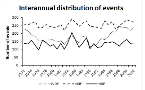
Figure 3.2 Interannual distribution of events. ……… 17
Figure 3.3 Seasonal climatology (1972 to 2002): of rainfall (a) of the amount of rainfall events (b). ………. 18
Figure 3.4 Interannual variation of the cases amount: DJF (a), MAM (b), JJA (c) e SON (d). ………... 19
Figure 3.5 Daily Interannual distribution of rainfall intensity: WRE (a), NRE (b) e HRE (c). ……… 20
Figure 4.1 (a) Spatial distribution rain gauges. (b) Seasonal climatology of precipitation. (c) Seasonal climatology of the amount of events. ……… 26
Figure 4.2 Distribution of daily precipitation mean of HRE, NRE and WRE. Parts (a), (c) and (e) have the rainier seasons (MAM and DJF). Parts (b), (d) and (f) have drier seasons (SON and JJA). In all figures interannual variation is presented. ……….….. 29
Figure 5.1 Spatial distribution rain gauges: (a) Northern coast (NC), (b) Northern semi-arid (NS), (c) Northwest (NW), (d) Southern semi-arid (SS), (e) Southern coast (SC). ………. 38
Figure 5.2 Annual climatology of precipitation for each sub-region. ……… 39
Figure 5.3 Daily precipitation mean, annual and seasonal, of the WRE. ………….. 40
Figure 5.4 Daily precipitation mean, annual and seasonal, of the NRE. …………... 41
Figure 5.5 Daily precipitation mean, annual and seasonal, of the HRE. …………... 42
Figure 5.6 Annual amount of the: WRE, NRE and HRE. ………. 44
Figure 5.7 Seasonal amount of the WRE. ……….. 45
Figure 5.8 Seasonal amount of the NRE. ………... 46
Figure 5.9 Seasonal amount of the HRE. …………...……… 47 Figure 5.10 Mann Kendall test for the variation annual of the WRE, NRE and HRE.
the × when there is no trend. The shading symbols represent positive trend and empty symbols represent negative trend. ………. 48 Figure 5.11 Mann Kendall test for the variation seasonal of the WRE. For each
sub-region there are two tags: the markup above is related to the amount of events and the marking below is related to intensity of the precipitation. The circles represent trends without statistical significance; triangles represent trends with statistical significance and the × when there is no trend. The shading symbols represent positive trend and empty symbols represent negative trend. ………... 49 Figure 5.12 As shown in figure 11, but for the NRE. ………. 50 Figure 5.13 As shown in figure 11, but for the HRE. ……….. 51 Figure 5.14 Area of the NEB that presents highest incidence of droughts. ………… 51 Figure 6.1 The rain gauge spatial distribution (black dots) over the NEB coastland. 55 Figure 6.2 Annual distribution of the number of HRE and precipitation intensity. .. 58 Figure 6.3 Geopotential anomaly (shading) and wind anomaly (vectors) at 200 hPa
and 850 hPa of North coastland: (a) dry season and (b) wet season. …... 59 Figure 6.4 Geopotential anomaly (shading) and wind anomaly (vectors) at 200 hPa
LISTA DE TABELAS
Pág. Tabela 2.1 Número de estações por estado e suas respectivas porcentagens: de
falhas, dias sem chuva e dias com chuva... 6 Table 3.1 Statistical significance (Sig.) and tendency (Tend.) of increase
(+) or decrease (-), from Mann-Kendall test applied in variation
of quantity Events. ………. 21
Table 3.2 Statistical significance (Sig.) and tendency (Tend.) of increase (+) or decrease (-), from Mann-Kendall test applied in variation of intensity of daily Rainfall. ………. 21 Table 4.1 Number of occurrence to HRE, NRE and WRE and the
occurrence of El Niño and La Niña events according to their intensity (weak, moderate or strong). ……… 30 Table 4.2 Trend Statistical of the Mann-Kendall test applied in variation of
quantity Events. ……….. 31
Table 4.3 Trend Statistical of the Mann-Kendall test applied in variation of
mean daily rainfall. ……… 31
Table 5.1 Rainfall mean (mm) of HRE by season to the subregions.
………..………... 43
LISTA DE SIGLAS E ABREVIAÇÕES
ANA Agência Nacional de Águas DJF December, January and February DOL Distúrbios Ondulatórios de Leste
ECMWF European Centre for Medium-Range Weather Forecasts EPI Eventos de Precipitação Intensa
EPF Eventos de Precipitação Fraca EPN Eventos de Precipitação Normal EWD Easterly Waves Disturbances
FS Front Systems
HRE Heavy Rainfall Events
IPCC Intergovernmental Panel on Climate Change ITCZ Intertropical Convergence Zone
JJA June, July, August LI Linhas de Instabilidade LN Litoral Norte
LS Litoral Sul
MAM March, April and May NC Northern Coast
NO Noroeste
NEB Nordeste do Brasil NRE Normal Rainfall Events NS Northern Semi-arid
NW Northwest
PDO Pacific Decadal Oscillation SACZ South Atlantic Convergence Zone SC Southern Coast
SF Sistemas Frontais SL Squall Lines SN Semiárido Norte
SON September, October and November
SS Semiárido Sul
SS Southern Semi-arid
ULCV Upper-level Cyclonic Vortex
WRE Week Rainfall Events
CAPÍTULO I
INTRODUÇÃO
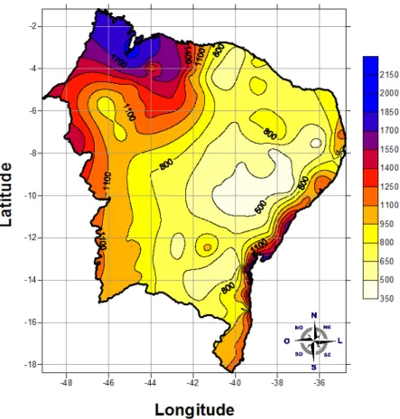
O Nordeste do Brasil (NEB) apresenta alta variabilidade climática abrangendo desde regiões semi-áridas, com precipitação anual acumulada inferior a 500 mm, até regiões com alto índice pluviométrico, como nas áreas costeiras e a noroeste da região, que apresentam precipitação anual superior a 1500 mm (Figura 1.1). Devido a sua grande extensão territorial são vários os sistemas meteorológicos atuantes no NEB, sendo os principais: a Zona de Convergência Intertropical (ZCIT), os Vórtices Ciclônicos de Altos Níveis (VCAN), os Distúrbios Ondulatórios de Leste (DOL), as Linhas de Instabilidade (LI), os Sistemas Frontais (SF) e a Zona de Convergência do Atlântico Sul (ZCAS), sendo os dois últimos atuantes sobre o sul da Bahia. Logo, os regimes de chuvas apresentam-se de forma heterogênea tanto na escala espacial quanto nas escalas de tempo.
Figura 1.1. Distribuição espacial da climatologia do total anual de precipitação (1972-2002). Fonte: Próprio autor, utilizando dados da ANA.
espacial e temporal de precipitação, acaba sendo afetada pela ocorrência de eventos extremos. Estes eventos extremos podem ser a sucessão de anos seguidos com chuvas abaixo do normal, caracterizando a seca (na escala climática) ou a ocorrência de eventos de precipitação intensa (EPI). Por ser mais comum a ocorrência de secas, esta já vem senda estudada por muitos; enquanto que sobre os EPI há poucos resultados na literatura especializada. Neste contexto, esta pesquisa objetivou analisar a tendência dos eventos de precipitação intensa sobre o NEB. A tese é composta por uma coletânea de artigos, os quais foram submetidos à medida que eram obtidos os resultados da pesquisa. Este primeiro capítulo é composto por: (1.1) Motivação, problemática e hipótese; (1.2) Objetivos e (1.3) Estrutura da tese.
1.1. Motivação, problemática e hipótese
A ocorrência de EPI causa grandes prejuízos sociais e econômicos às regiões atingidas. Investigações científicas no âmbito da modelagem climática sugerem que as mudanças no clima atual estão resultando em EPI mais frequentes e que a interferência do homem no meio ambiente vem intensificando as consequências destes eventos, com ações como o desmatamento de encostas e a construção civil em áreas de risco (Marengo, 2009). Porém, estimativas confiáveis de tendências para EPI são possíveis apenas para regiões com número considerável de estações meteorológicas. A falta de observações de longo prazo e de alta qualidade, ou seja, homogêneas, é o maior obstáculo para a quantificação das mudanças extremas durante o século passado (Vincent et al., 2005; Haylock et al., 2006). Esta falta de dados qualificados é também um dos obstáculos para a realização de estudos sobre estes eventos no NEB, tornando alguns resultados pouco consistentes.
Além da importância na análise do comportamento dos EPI em relação ao tempo, também é importante conhecer os fatores que antecedem sua formação, ou seja, conhecer as condições dinâmicas que favorecem o desenvolvimento e manutenção destes eventos, caracterizar o ambiente sinótico associado aos EPI. Com esta finalidade, alguns estudos vêm sendo desenvolvidos (Teixeira e Satyamurty, 2007; Lima et al., 2010; Liebmann et al., 2011) através da obtenção de anomalias de compostos de variáveis atmosféricas. Para um melhor resultado torna-se imprescindível o cálculo das anomalias também para os eventos de precipitação normal (EPN) e de precipitação fraca (EPF), para comparar os resultados dos campos das anomalias entre os eventos normais e os eventos intensos.
Um estudo observacional sobre EPI no NEB, com quantidade considerável de dados de precipitação que apresentem boa qualidade é inexistente, não há informações sobre sua climatologia, tendência, áreas preferenciais de ocorrência, características de formação, desenvolvimento e dissipação. Nesta pesquisa foram utilizadas 151 estações pluviométricas, apresentando 5,91% de falhas. Um maior detalhamento sobre as estações utilizadas se encontra no apêndice A.
No entanto, como dito anteriormente, os EPI sobre o NEB são pouco estudados mesmo causando grandes prejuízos à população; portanto, acredita-se que se faz necessário um estudo mais abrangente sobre esses eventos. Neste contexto, a presente pesquisa foi realizada no intuito de responder duas questões principais:
i) Os EPI no NEB apresentam tendência em relação à quantidade de ocorrência e a intensidade da precipitação?
ii) Qual a relação entre a variabilidade dos eventos de precipitação fraca, normal e intensa?
As hipóteses para responder a essas questões são:
i) Visto que resultados através de modelagem computacional mostram alterações no ciclo hidrológico em diversas regiões, incluindo o NEB, e também, em grande parte, aumento na quantidade de eventos extremos, então é provável que os eventos intensos de precipitação possam ter tendência, ou então estarem associados à variabilidade da atmosfera;
ii) Se o evento de precipitação intensa apresentar tendência, provavelmente isto ocasionará uma alteração no regime de chuvas da região, logo este resultado irá refletir sobre os demais eventos de precipitação, podendo haver uma relação direta ou inversa entre os diferentes tipos de eventos.
1.2. Objetivos
O objetivo geral da pesquisa é determinar a climatologia e identificar a tendência dos eventos de precipitação intensa sobre o NEB e compará-los aos eventos de precipitação normal e fraca.
Os objetivos específicos deste estudo são:
Determinar os eventos de precipitação fraca, normal e intensa;
Delimitar sub-regiões climatologicamente homogêneas sobre o NEB;
Analisar a climatologia, a tendência interanual e sazonal da quantidade e da média diária de precipitação dos eventos, nas sub-regiões;
Caracterizar o ambiente sinótico associado aos EPI, definindo os regimes meteorológicos responsáveis por ocasioná-los.
1.3. Estrutura da tese
Esta tese é composta por seis capítulos, sendo que o capítulo 2 é composto por um capítulo de livro publicado, os capítulos 3 e 5 apresentam artigos publicados em periódicos, o capítulo 4 é formado por um artigo submetido a periódico e as considerações finais da tese são mostradas no capítulo 6.
A publicação dos artigos aconteceu conforme a evolução da pesquisa. Inicialmente, a obtenção dos dados junto a Agência Nacional de Águas (ANA) foi um pouco demorada, de forma que foram recebidos os dados referentes a todos os estados do NEB, com exceção da Bahia. Então, iniciou-se a análise com os dados disponíveis e foram obtidos resultados interessantes. Neste período surgiu a oportunidade de elaborar um capítulo para o livro Rainfall: Behavior, Forecasting and Distribution, como já se tinha os resultados prontos, elaborou-se o capítulo o qual foi publicado. Com o recebimento dos dados referentes ao Estado da Bahia, foi realizada uma nova análise para todo o conjunto de dados do NEB, os resultados deram origem a um artigo publicado na Atmospheric Science Letters. Após a análise da tendência em todo o NEB, realizou-se o estudo da tendência em suas sub-regiões climatologicamente homogêneas, resultando em um novo artigo que foi submetido à
International Journal of Climatology. Após a obtenção da tendência realizou-se a análise do ambiente sinótico associado aos EPI para as sub-regiões do litoral, sendo publicado um novo artigo na Advances in Geosciences. Cronologicamente, este foi o primeiro artigo a ser publicado, pois a elaboração e publicação do mesmo foi mais rápida que os demais artigos. Na sequência são apresentadas as publicações que deram origem aos capítulos:
Capítulo 3 - Oliveira, P. T.; Santos e Silva, C. M.; Lima, K. C. Linear trend of occurrence and intensity of heavy rainfall events on Northeast Brazil. Atmospheric Science Letters, 2014. DOI:10.1002/asl2.484.
Qualis CAPES: A1 – Interdisciplinar / B1 – Geociências
Capítulo 4 - Oliveira, P. T.; Santos Silva, C. M.; Lima, K. C. Trend analysis of extreme precipitation in sub-regions of Northeast Brazil. Artigo pronto para submissão.
Capítulo 5 - Oliveira, P.T.; Santos e Silva, C. M.; Lima, K. C. Synoptic environment associated with heavy rainfall events on the coastland of Northeast Brazil. Advances in Geosciences, v. 35, p. 73-78, 2013.
Qualis capes: B2 – Interdisciplinar / B3 – Geociências
CAPÍTULO 2
DADOS E METODOLOGIA
2.1. Dados
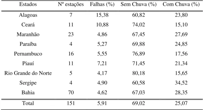
Foram utilizados os dados diários de precipitação da rede hidrometeorológica gerenciada pela ANA, contabilizando 349 estações. Os dados recebidos passaram por uma série de etapas a fim de serem organizados e filtrados até chegarem à melhor forma de serem utilizados. Na filtragem considerou-se a quantidade de falhas em cada estação. Como alguns estados apresentaram maior quantidade de falhas que outros, a filtragem foi realizada por estado, pois cada um apresentou um diferente nível aceitável. Por exemplo, as estações do estado de Alagoas apresentavam altos níveis de falhas, então ao selecionarmos as estações com melhor qualidade dos dados foi aceitável uma falha de 15,38%, pois se não fosse assim não seria possível utilizar os dados deste estado.
Após a verificação da qualidade dos dados das 349 estações obtidas, foram escolhidas 151 estações para o período de 1972 a 2002, por ser este o período que apresentou dados mais consistentes.
O resultado desta filtragem pode ser conferido na Tabela 2.1. As estações escolhidas estão distribuídas de acordo com a Figura 2.1.
Tabela 2.1 – Número de estações por estado e suas respectivas porcentagens: de falhas, dias sem chuva e dias com chuva.
Estados Nº estações Falhas (%) Sem Chuva (%) Com Chuva (%)
Alagoas 7 15,38 60,82 23,80
Ceará 11 10,88 74,02 15,10
Maranhão 23 4,86 67,45 27,69
Paraíba 4 5,27 69,88 24,85
Pernambuco 16 5,55 76,89 17,56
Piauí 11 7,21 71,45 21,34
Rio Grande do Norte 5 4,17 80,18 15,65
Sergipe 4 4,90 60,58 34,52
Bahia 70 4,62 67,03 28,35
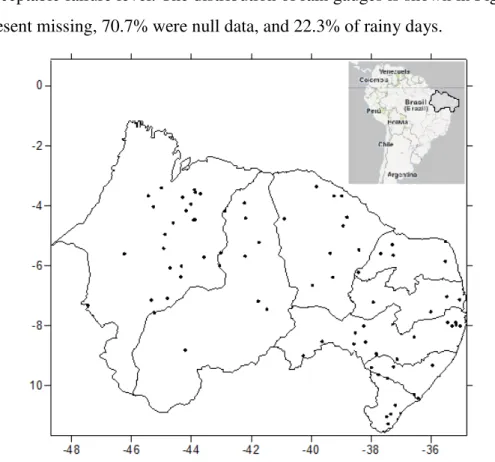
Figura 2.1 – Distribuição espacial das estações utilizadas
Para caracterizar o ambiente sinótico associado aos EPI foram utilizados os dados diários de reanálises do projeto ERA Interim (Dee et al., 2011), do European Centre for Medium-Range Weather Forecasts (ECMWF). O ERA-Interim é a mais recente reanálise atmosférica global produzida pelo ECMWF, o qual abrange o período de 01 de janeiro de 1979 até a data atual e apresenta espaçamento de grade de 1,5º latitude x 1,5º longitude. As variáveis meteorológicas utilizadas foram: Umidade específica, Vento zonal, Vento meridional e o Geopotencial, para o período de 1979 a 2002.
2.2. Metodologia
2.2.1. Técnica dos quantis
Os quantis são pontos tomados a intervalos regulares de uma série de dados, dividindo-a em subconjuntos de mesmo tamanho. Os principais quantis são: os quartis, que dividem a série de dados em quatro partes iguais; os decis, que dividem a série de dados em dez partes iguais; os percentis, que dividem a série de dados em cem partes iguais (Martins, 2005).
padrão, é que este último é fortemente dependente da hipótese da normalidade da distribuição da precipitação, hipótese não necessariamente satisfeita em grande parte das séries disponíveis.
Neste estudo além dos EPI, também foram calculados os EPF e os EPN, todos com base no cálculo dos percentis da distribuição de precipitação, considerando apenas os dados de dias com chuva acima de zero. Definiu-se como EPI aquele que apresentou precipitação acima do percentil 95º; como EPN aquele que apresentou precipitação em torno do valor médio, ou seja, entre o percentil 45º e 55º; e como EPF aquele que apresentou precipitação abaixo do percentil 5º. Desta forma, foram calculados os percentis e definidos os eventos de precipitação em cada posto pluviométrico. Posteriormente, os resultados foram organizados, por tipo de evento de precipitação, onde calculou-se a quantidade de EPF, EPN e EPI e a intensidade da precipitação média diária destes eventos, durante o período de estudo (1972 a 2002).
A quantidade e a intensidade dos EPF, EPN e EPI foram analisadas anual e sazonalmente, sendo as estações definidas como: verão, DJF (Dezembro, Janeiro e Fevereiro); outono, MAM (Março, Abril e Maio); inverno, JJA (Junho, Julho e Agosto); primavera, SON (Setembro, Outubro e Novembro).
2.2.2. Análise de tendência
Aplicou-se o teste de Mann-Kendall para analisar a tendência de variação na quantidade de eventos e na intensidade da precipitação. Este teste é classificado como não-paramétrico (Mann, 1945; Kendall, 1975) e consiste em comparar cada valor da série temporal com os valores restantes, sempre em ordem sequencial, contando o número de vezes em que os termos restantes são maiores que o valor analisado. O teste de Mann Kendall é calculado como a seguir:
O valor de S é obtido pela soma de todas as contagens da série de dados, sendo e os valores da série (anual ou sazonal) nos anos i e j, respectivamente.
(2.1)
sendo o sinal obtido da seguinte forma:
quando n é muito grande, o valor de S tende para a normalidade com variância definida como:
(2.2)
em que é o número de dados com valores iguais em certo grupo e o número de grupos contendo valores iguais na série de dados em um grupo . Finalmente, o teste estatístico de Mann Kendall é dado pela seguinte equação:
(2.3)
Através do valor de , determina-se a tendência estatisticamente significativa na série temporal. Para testar qualquer tendência (positiva ou negativa) para determinado nível de significância, a hipótese nula é aceita se Z é menor que
, que é obtido na tabela normal,
logo um valor positivo de indica tendência crescente, enquanto que um valor negativo de
indica tendência decrescente. Neste trabalho utilizou-se os níveis de significância de α = 0,001; α = 0,01; α = 0,05; α = 0,1.
Para aplicação do teste de Mann- Kendall, utilizou-se a planilha MAKESENS, desenvolvida por Salmi et al. (2002).
2.2.3. Análise de cluster
A análise de agrupamento, ou análise de clusters, é o processo de agrupar um conjunto de objetos em classes de objetos similares. A criação de uma divisão dos elementos deverá ter como característica a homogeneidade dos elementos que se inserem em cada grupo. Uma noção fundamental na análise de agrupamento é a noção de semelhança e/ou de dessemelhança entre os casos a agrupar, pois se pretende que os elementos de um grupo sejam os mais semelhantes possíveis e que os elementos de dois grupos distintos sejam os mais dessemelhantes possíveis.
métrica. Na presente pesquisa utilizou-se como medida de similaridade a distância euclidiana, que é determinada pela seguinte equação:
(2.4)
em que e são os elementos a serem comparados, sendo o índice representante da quantidade de grupos e os índices e representantes dos elementos do grupo.
Os métodos utilizados na análise de cluster apresentam-se em duas classes, os hierárquicos e os não- hierárquicos, aqui utilizaremos um método hierárquico. Este método consiste em uma série de sucessivos agrupamentos ou sucessivas divisões de elementos, onde os elementos são agregados ou desagregados. Estes grupos são geralmente representados por um diagrama bi-dimensional chamado de dendrograma ou diagrama de árvore. Neste diagrama, cada ramo representa um elemento, enquanto a raiz representa o agrupamento de todos os elementos. Através do dendrograma e do conhecimento prévio sobre a estrutura dos dados, deve-se determinar uma distância de corte para definir quais serão os grupos formados. Essa decisão é subjetiva, e deve ser feita de acordo o objetivo da análise e o número de grupos desejados. O método hierárquico é subdividido em métodos aglomerativos e divisivos, aqui utilizou-se o método de Ward. No método aglomerativo, cada elemento inicia-se representando um grupo e a cada passo um grupo ou elemento é ligado a outro de acordo com sua similaridade até o último passo, onde um grupo único com todos os elementos é formado. O método de Ward busca unir objetos que tornem os agrupamentos formados o mais homogêneo possível. A medida de homogeneidade utilizada baseia-se na partição da soma de quadrados total de uma análise de variância, descrita pela seguinte equação:
(2.5)
em que e representa os grupos.
Este método é bastante utilizado por basear-se numa medida com alta relevância estatística e por gerar grupos que possuem alta homogeneidade interna.
2.2.4. Anomalia da composição
três dias precedentes, identificando-se as características dinâmicas e sinóticas associadas aos episódios. Um campo composto de uma dada variável é obtido da seguinte maneira:
(2.6)
em que é a variável do composto, (x, y, p) indica a posição espacial da variável, N é o número de casos identificados durante o período de estudo, D-n é o nésimo dia precedente ao evento (n = 0, 1, 2, 3), e o sufixo j refere-se ao jésimo evento.
Para representar a climatologia da variável temos ; portanto, a anomalia da composição é definida como:
CAPÍTULO 3
TREND OF RAIN IN NORTHEAST BRAZIL
(Tendência de chuvas no Nordeste do Brasil)
RESUMO
O Nordeste do Brasil (NEB) apresenta alta variabilidade no clima, abrangendo desde regiões semi-áridas, com precipitação anual acumulada inferior a 500 mm, até climas chuvosos nas regiões costeiras, que apresentam precipitação anual superior a 1500 mm. Os regimes de chuvas apresentam-se de forma heterogênea tanto na escala espacial quanto nas escalas de tempo. Segundo o último relatório do Intergovernmental Panel on Climate Change (IPCC; AR4), o NEB é uma região altamente susceptível às mudanças climáticas, além de ser uma região sujeita à ocorrência de eventos de precipitação intensa (EPI) extrema; contudo, ainda existem poucos estudos sobre a climatologia destes episódios nesta região. Neste sentido, o objetivo do trabalho foi determinar a climatologia do número de eventos e da taxa diária de precipitação associadas aos EPI, relacionando-os aos eventos de precipitação normal (EPN) e de precipitação fraca (EPF). Foram analisados oito estados do NEB, excluindo-se a Bahia, devido seu diferente regime pluviométrico. Utilizaram-se os dados diários de precipitação da rede hidrometeorológica gerenciada pela Agência Nacional de Águas (ANA) para o período de 1972 a 2002 (31 anos), totalizando 219 pluviômetros. Para identificar os eventos foi aplicada a técnica dos quantis. Selecionaram-se os EPI, EPN e EPF quando pelo menos um pluviômetro registrou precipitação acima do percentil 95°, entre os percentis 45º e 55º, e abaixo do percentil 5º, respectivamente. A distribuição dos dados referentes aos eventos foi dividida por estação sazonal (DJF, MAM, JJA, SON). Aplicou-se o teste de Mann-Kendall a fim de analisar a tendência linear do número de eventos e da taxa diária de precipitação anual de cada classe. Verificou-se aumento do número de casos e da intensidade da precipitação nos EPF e de intensidade nos EPI em níveis acima de 95% de confiança estatística. Por outro lado, os EPN apresentaram diminuição na intensidade dos casos no trimestre JJA (período seco). Os resultados sugerem que as mudanças climáticas estão alterando a climatologia de chuvas do NEB, intensificando os eventos extremos (intensos e fracos) e enfraquecendo os eventos médios, mais especificamente intensificando os EPI durante a época chuvosa.
TREND OF RAIN IN NORTHEAST BRAZIL
3.1. Introduction
Northeast Brazil (NEB) is composed by Alagoas, Bahia, Ceará, Maranhão, Paraíba, Pernambuco, Piauí, Rio Grande do Norte and Sergipe Brazilian states, occupying 1,588,196 km², which is equivalent to 18% of the Brazilian territory, situated between 1ºN and 18ºS and 34.5ºW and 48.5ºW. The NEB presents a high climatic variety since semi-arid regions (annual rainfall less than 500 mm), reaching the coastland (annual precipitation above 1500 mm), being influenced by extreme events on the time scale (precipitation excess) and climatic scale (dry episodes). The rainfall presents itself heterogeneously in the spatial-temporal scales. The main atmospheric systems acting in the NEB are: the Intertropical Convergence Zone (ITCZ); the Upper Tropospheric Cyclonic Vortex (UTCV); the Easterly Waves Disturbances (EWD) and the Squall Lines (SL). The South of Bahia has actuation of the Front Systems (FS) and the South Atlantic Convergence Zone (SACZ). Specifically, the Semi-arid Northeast study verified that intense events are associated to mesoscale systems, which are embedded in dynamic-unstable synoptic environments (Barbosa e Correia 2005; Diniz et al. 2004; Silva et al. 2008).
The ITCZ is an atmospheric system located around the globe equatorial line, formatted by confluence between the northeast and southeast trade winds. The ITCZ showed a northsouth displacement through the year, reaching maxima latitude around at 1º S (April), and 8º N (July), this variability to determinate the rainy and dry periods over the north NEB (Uvo, 1989).
According to Kayano et al. (1997) the UTCV are systems with a persistent and cold core, which influence the rainfall during the austral summer time in NEB. In the core the motion is descending, inhibiting the generation of clouds and in the UTCV periphery the wet air motion is ascending, causing potential kinetic energy conversion and keeping the UTCV motion (Gan and Kousky, 1986).
The SL‘s are agglomerated of cumulus clouds organized in line shape, associated to the sea breeze (Kousky, 1980; Cavalcanti, 1982; Cohen, 1989; Greco et al., 1990). Due to diurnal variability, the maxima convective activity occurs at late afternoon hours, being often observed in infrared satellite images.
System Front (SF) is the region that presents two air masses with different characteristics. The cold air mass advances over the given region, causing hot air to ascend. During the austral winter, these systems are formed by air masses originated from high latitudes, causing frost and rainfall episodes in different parts of Brazil, including the South NEB. During the cold fronts moving toward low latitudes, they interact with air producing hot and moist tropical deep convection (Cavalcanti and Kousky, 2009). The interaction between the FS and the convection due to the diabatic heating at the surface organizes a preferential region of convergence (SACZ) especially during the summer months. The SACZ is characterized by a band of cloudiness with a northwest-southeast orientation that extends from the Amazonia southwest to the Atlantic Ocean (Kodama, 1992). The SACZ presents a stationary characteristic, with a period of four or more days above the same region.
Although the different actuating atmospheric systems above all the NEB, the most climatologically rainy period occurs during the fall, on March, April and May (Silva, 2004). According to the last report from the Intergovernmental Panel on Climate Change (IPCC; AR4), the NEB is an area highly susceptible to climatic changes, being susceptible to the occurrence of high precipitation events. An important question about these extreme events is the time tendency identification.
The climatic change influences the intensity and frequency extreme events depending not only on the rate of change of the environment variable, but of the statistical parameter changes that determine the variable distribution. The analysis of extreme precipitation is the most complex analyses, due to the low degree of correlation between the precipitation events (Marengo, 2009).
The reliable tendencies estimative of the precipitation events are possible in areas with a dense rain gauge dataset. The lack of high quality and homogeny weather observations is the greatest obstacle to quantify the extreme changes during the past century (Vincent et al., 2005, Haylock et al., 2006).
nonexistent, having only results in global studies that involve the region (Groisman et al., 2005; Marengo et al., 2009).
The objective of this study regards the climatology and the tendency toward the number of events and the daily precipitation rate associated with Heavy Rainfall Events (HRE), Normal Rainfall Events (NRE) and Weak Rainfall Events (WRE).
3.2. Material and methods
3.2.1. Data
This study was performed with a rainfall dataset of the eight NEB states: Alagoas, Ceará, Maranhão, Paraíba, Pernambuco, Piauí, Rio Grande do Norte and Sergipe.
The Bahia was excluded due to its different rainfall regime. Daily precipitation data of the hydrometeorological network management by the National Water Agency of Brazil (Agência Nacional de Águas - ANA) was used. This included an accounting from 219 stations during the period from 1972 to 2002 (31 years).
A quality control was made to exclude spurious and missing data, thus only 81 rain gauges presented acceptable failure level. The distribution of rain gauges is shown in Figure 3.1. This total, 7% present missing, 70.7% were null data, and 22.3% of rainy days.
3.2.2. Methodology
3.2.2.1. Quantiles Technique
The quantiles are points in regular intervals of a series of data. According to Wilks (2006), many statistical analyses were based on the quantiles technique. The main advantage of this technique with relation to the traditional methods (mean and standard deviation) is the independency on normalization hypothesis, which is not necessarily satisfied in rainfall data. In addition, the quantiles technique considers the characteristic of the precipitation distribution frequency of each meteorological station. Therefore, the quantiles are immune to eventual asymmetry on the density function of probabilities that describes a random phenomenon (Xavier, 1984).
To determine extreme events, many studies were developed in different regions, using the distribution of daily rainfall percentiles. Groisman et al. (2005) used the 90th, 95th, 99th, 99.7th and 99.9th percentiles in a global study, Zhai et al. (2005) applied the 95th percentile to China rainfall; Grimm and Tedeschi (2009) performed a study over South America, using the 90th percentile; Khishnamurthy et al. (2009) identified extreme events in the region of India from the 90th and 99th percentiles; Jones et al. (2011) used the 90th percentile in a study over the USA; finally, Gemmer et al. (2011), with rainfall data over China used the 90th, 95th and 99th percentiles.
In the present study we select extreme (weak and intense events) and the normal events only to nonzero daily rainfall. Each case is selected if at least one rain gauge was observed: Heavy Rainfall Event (HRE) presented precipitation great than 95th percentile; the Normal Rainfall Event (NRE), are between percentiles 45th and 55th; Week Rainfall Event (WRE) presented precipitation less than 5th percentile. The data was divided by seasons: summer DJF (December, January and February); autumn MAM (March, April and May); winter JJA (June, July, August); spring SON (September, October and November).
3.2.2.2. Trend Analyses
3.3. Results and discussion
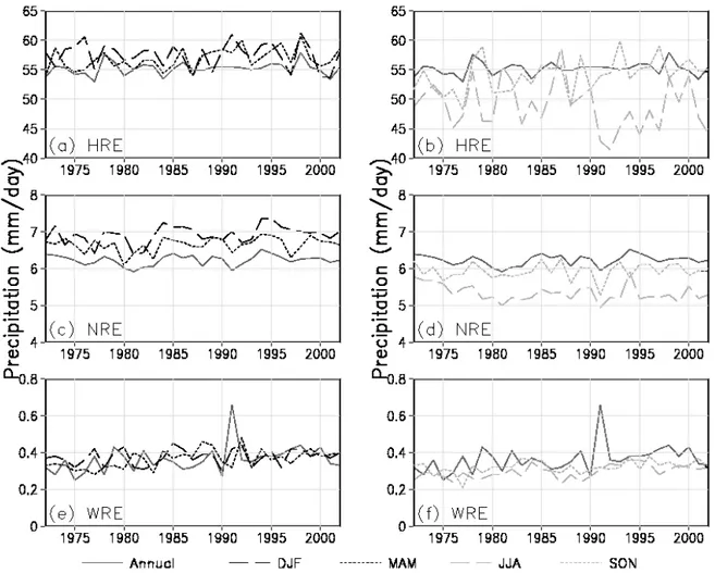
Figure 3.2 presents the annual distribution of rainfall events during the studied period. Both NRE and HRE show a cyclic and correspondent variability. It is not possible to identify linear trends in this data. The year with maxima quantity of NRE and HRE were 1985, 1989 and 2000; and minimum quantity in 1976, 1981, 1983, 1993 and 1997, coincided with strong La Niña and El Niño events, respectively. According to Grimm and Tedeschi (2009) and Rodrigues et al. (2011), El Niño and La Niña events have direct influence on the NEB rainy season, and consequently on the NRE and HRE. During El Niño years the NRE and HRE events decrease, while in La Niña they increase; however, the El Niño actuation is more pronounced than La Niña events. The WRE do not present cyclic characteristics and the data presents a linear decrease from 1972 until 1982. Between 1983 and 1990 the distribution of WRE strongly corresponds to the variation of the NRE and HRE (El Niño and La Niña events). After 1990 the number of events increases significantly.
The seasonal climatology of rainfall is presented in Figure 3.3(a). The period of highest rainfall is during autumn (MAM) and the minimum is in the spring (SON). Comparing with WRE, NRE and HRE seasonal climatology (Figure 3.3(b)) it is possible to verify consistent distributions. The HRE seasonal variation is more accentuated than the WRE and NRE one. The dry seasons (JJA and SON) contain fewer HRE in comparison with other events.
The interannual variation of the WRE, NRE and HRE is described in Figure 3.4. In Figure 3.4(a) it shows the distribution of summer Events, where after 1993 presents a positive trend. The same occurs during MAM for the WRE and NRE (Figure 2.4(b)), with exception of the HRE, which shows no trend in the study period. During the winter and spring the variability of NRE and HRE do not present significant trends, whereas the WRE presents a positive trend.
Figure 3.3. Seasonal climatology (1972 to 2002): of rainfall (a) of the amount of rainfall events (b).
Figure 3.5 shows the daily interannual distribution of rainfall intensity. The WRE (Figure 3.5(a)) presents a strong positive trend for all seasons. In general, The NRE, Figure 3.5(b), shows no positive or negative trend, with the exception of the winter season (JJA), which shows a negative trend. The HRE, Figure 3.5(c), does not show a relevant trend, except during MAM, which shows a positive trend. The intensity variability is also correlated with El Niño and La Niña occurrences, but this variation is less sensitive to these phenomena than the variation in the number of events.
NRE and HRE presented positive tendency during all seasons, except for DJF and MAM, which showed a positive trend for NRE and HRE, respectively, but without statistical significance.
Figure 3.5. Daily Interannual distribution of rainfall intensity: WRE (a), NRE (b) e HRE (c).
al. (2005), who observed in the east of Brazil (almost all the NEB), there was an increase of 40% in the HRE annual frequency in the period between 1910 and 2000, however their results were statistically significant at 10%.
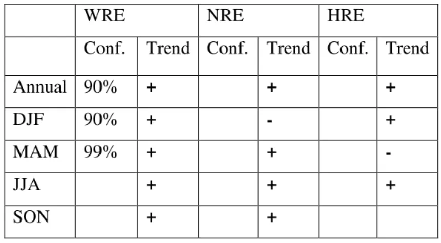
Table 3.1. Statistical confidence (Sig.) and tendency (Tend.) of increase (+) or decrease (-), from Mann-Kendall test applied in variation of quantity Events.
WRE NRE HRE
Conf. Trend Conf. Trend Conf. Trend
Annual 90% + + +
DJF 90% + - +
MAM 99% + + -
JJA + + +
SON + +
Table 3.2. Statistical confidence (Sig.) and tendency (Tend.) of increase (+) or decrease (-), from Mann-Kendall test applied in variation of intensity of daily Rainfall.
WRE NRE HRE
Conf. Trend Conf. Trend Conf. Trend Annual 99.9% + 95% -
DJF 90% + - -
MAM 99% + - 95% +
JJA 99% + 95% -
SON 90% + - +
3.4. Conclusion
A set of 81 rain gauges distributed over the NEB provided daily rainfall data, which were used to analyze the WRE, NRE and HRE. The main objective was to calculate the climatology of the number of cases and daily rainfall rate associated with these events.
CAPÍTULO 4
LINEAR TREND OF OCCURRENCE AND INTENSITY OF HEAVY RAINFALL EVENTS ON NORTHEAST BRAZIL
(Tendência linear da quantidade e intensidade dos eventos de precipitação intensa no Nordeste do Brasil)
RESUMO
Dados diários obsercados de precipitação para o período de 1972 a 2002, foram utilizados para calcular a climatologia e a tendência de ocorrência e intensidade de eventos de precipitação fraca, normal e intensa no Nordeste do Brasil. Os eventos foram definidos utilizadando a técnica dos quantis e a tendência foi identificada pelo teste de Mann -Kendall. Os eventos intensos foram modulados pelas ocorrências de La Niña e El Niño e, em geral, apresentaram tendência negativa em relação à quantidade e tendência positiva em relação à intensidade.
LINEAR TREND OF OCCURRENCE AND INTENSITY OF HEAVY RAINFALL EVENTS ON NORTHEAST BRAZIL
4.1. Introduction
The Northeast Brazil (NEB) exhibits high climatic variety since semi-arid regions (annual rainfall less than 500 mm), to rainy regions in the coastland (annual precipitation above 1500 mm), being influenced by extreme events on the weather scale (precipitation excess) and climatic scale (dry episodes). The rainfall observed is heterogeneous in the spatial-temporal scales due the main atmospheric systems that act in NEB: the Intertropical Convergence Zone (ITCZ) (Coelho et al., 2004); the Upper Tropospheric Cyclonic Vortex (Kousky and Gan, 1981); the Easterly Waves Disturbances (EWD) (Riehl, 1945) and the Squall Lines (SL) (Kousky, 1980). The South Bahia has actuation from the Front Systems (FS) (Kousky, 1979) and the South Atlantic Convergence Zone (SACZ) (Kodama, 1992). Climatologically the rainy season occurs during the autumn (March-April-May) (Silva, 2004), although the variety of atmospheric systems above all the NEB.
Several studies focusing on the climatological aspects of rainfall in NEB exist, but, studies concerning heavy rainfall events (HRE), with considerable amount of rainfall data of good quality, have been scarce. There are little insights about climatology, trends, preferred areas of occurrence, characteristics of the formation, development and dissipation of HRE. Knowing the climatology of these events provide important informations that can be used for predictability purposes.
A trend analysis of extreme events of precipitation is very complex because there is a low degree of temporal and spatial correlation between the precipitation events. Despite the difficulty, several studies were conducted in order to understand how far the anthropogenic changes have interfered on the occurrence of these events. For example, studies were conducted in China (Gemmer et al., 2011), Iberian Peninsula (Acero et al., 2011), United States of America (Santos et al., 2011), Central Asia (Bothe et al., 2011) and Europe (Anagnostopoulou and Tolika, 2012).
(Haylock et al., 2006; Groisman et al., 2005); however, there are evidences of positive trends of HRE occurrence on NEB.
Thus, the objective of this study is to verify the general behavior of HRE on NEB relating them to the Normal Rainfall Events (NRE) and Weak Rainfall Events (WRE) by analyzing the variability and trends of these events in respect to the number of occurrence and intensity of the rainfall.
4.2. Methodology
4.2.1. Datasets
A comprehensive dataset of daily precipitation obtained from the 349 rain gauges management by the National Water Agency of Brazil (Agência Nacional de Águas - ANA) was used. The data covers from 01 January 1972 to 31 December 2002 (31 years) period. These data have undergone a process of quality control, resulting in 151 stations with 5.91% of missing data. The stations used are distributed according to Figure 4.1(a). In recent work, Oliveira et al. (2012) analyzed the variability of precipitation and HRE on NEB; though, your analysis excluded the dataset of Bahia State, therefore in Oliveira et al. (2012) the total of rain gauges is 80.
4.2.2. Quantiles Technique
The quantiles are points of a series of data organized in regular intervals. According to Wilks (2006) many statistical analyses were based on the quantiles technique. The main advantage of this technique in relation to the traditional methods (mean and standard deviation) is the independency on normalization hypothesis, which is not necessarily satisfied in daily rainfall data. In addition, the quantiles technique considers the frequency distribution of precipitation to each rain gauge data. Therefore, the quantiles are immune to eventual asymmetry on the density function of probabilities that describes a random phenomenon.
Figure 4.1. (a) Spatial distribution rain gauges. (b) Seasonal climatology of precipitation. (c) Seasonal climatology of the amount of events.
In the present study we selected extreme (weak and intense events) and the normal events only to nonzero daily rainfall. Each case is selected if at least one rain gauge was observed, based on previous works (Liebmann et al., 2001; Carvalho et al., 2002), thus: (1) the HRE presented precipitation ≥ 95th percentile; (2) the NRE is identifying when the daily precipitation is between percentiles 45th and 55th; (3) the WRE presented precipitation ≤ 5th percentile. The dataset analyses was divided by seasons: summer DJF (December, January and February); autumn MAM (March, April and May); winter JJA (June, July, August); spring SON (September, October and November).
4. 2.3. Trend Analyses
and Cherkauer, 2008; Santos et al., 2010; Acero et al. 2011). To apply the Mann-Kendall test, the MAKESENS spreadsheet developed by Salmi et al. (2002) was used, the calculations are performed as follows.
The S value is obtained by summing the counts of all the data series, and are the values of the series and i, j the years, being i = j+1.
(4.1)
The signal function is performed as follows:
To high values of n , the S parameter tends to normality with variance defined as:
(4.2)
where is the number of data with equal values into the certain group, and the number of groups having equal values in the series of data in one group . Finally, the Z value of the Mann Kendall test is determinated by the following equation:
(4.3)
The value determines the statistically significant of trend. To test any trend (positive or negative) for a given level of significance, the null hypothesis is accepted if the value of Z is less than
, which obtained from the standard normal cumulative distribution tables,
then a positive indicates positive trend, while a negative value of indicates a negative trend. In this paper we use the following significance levels: α = 0.001; α = 0.01; α
4.3. Results and discussion
In the Figure 4.1(b) the seasonal climatology of rainfall is presented. The autumn (MAM) is the main rainy season with maximum precipitation of 400 mm and the dry season is the spring (SON) when the precipitation reaches 100 mm. The distribution of HRE, NRE and WRE (Figure 4.1(c)) is consistent with the rainfall climatology. The number of HRE, NRE and WRE occurrence is higher in MAM, but the distribution is relatively different. The NRE and WRE are ranging from 2000 to 2600 events whereas the HRE are concentrated in DJF and MAM seasons. However, the HRE in JJA and SON is about 1000 cases resulting in an annual mean of 33 cases during the dry seasons and 65 cases in rainy seasons.
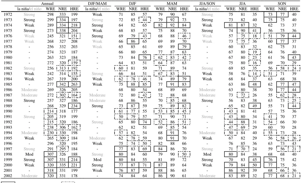
Table 4.1 shows the number of occurrence to HRE, NRE and WRE, annually and seasonally, and the occurrence of El Niño and La Niña events according to their intensity (weak, moderate or strong). The years with maximum occurrence of HRE were 1974, 1985, 1989, 1999 and 2000 and minimum in 1976, 1981, 1983, 1987 and 1993. Concerning the NRE, the years with maximum were 1973, 1974, 1975, 1985 and 2000, and minimum in 1982, 1987, 1993, 1995 and 1997. The years with maximum occurrence of WRE were 1998, 1999, 2000, 2001 and 2002 and minimum in 1990, 1991 1992, 1993 and 1994. The maximum and minimum occurrence of HRE, NRE and NRE coincide to years of La Niña and El Niño, respectively. According to Coelho et al. (2002), Grimm and Tedeschi (2009) and Rodrigues et al. (2011), El Niño and La Niña events have direct influence on the NEB rainy season and consequently on the HRE, NRE and WRE. For all seasons, the number of HRE showed low variability with negative trend from 1972 to 1991 and positive trend after 1991. However, this behavior is not observed respecting to NRE and WRE, expect to the WRE during the DJF. The precipitation intensity of HRE, NRE and WRE is presented in Figure 3.2. The HRE shows variation between 54 and 62 mm day-1 (Figure 4.2(a)) to the rainy seasons, DJF and MAM. During dry seasons, JJA and SON, the rain rate varies between 41 and 60 mm/day (Figure 4.2(b)). The annual variation is between 53 and 58 mm day-1. There is a higher amplitude for the dry period which reaches 17 mm day-1 in JJA, with maximum in 1987 (59 mm day-1) and minimum in 1992 (41 mm day-1), whereas in the rainy season reaches a maximum amplitude of only 8 mm day-1, it is perceived that the dry season has more variability relatively to the rainy one.
season (JJA), which shows a negative trend. The difference between the maximum and minimum WRE intensity during rainy and dry seasons do not exceeds 0.2 mm day-1; however presents a significant positive trend for all seasons. The intensity variability is correlated with El Niño and La Niña occurrences, but this variation is less sensitive to these phenomena than the variation in the number of events.
Figure 4.2. Distribution of daily precipitation mean of HRE, NRE and WRE. Parts (a), (c) and (e) have the rainier seasons (MAM and DJF). Parts (b), (d) and (f) have drier seasons (SON and JJA).
In all figures interannual variation is presented.
Table 4.1. Number of occurrence to HRE, NRE and WRE and the occurrence of El Niño and La Niña events according to their intensity (weak, moderate or strong).
Annual DJF/MAM DJF MAM JJA/SON JJA SON
la niña/el niño WRE NRE HRE la niña/el niño WRE NRE HRE WRE NRE HRE la niña/el niño WRE NRE HRE WRE NRE HRE
1972 Strong 298 333 199 Weak 71 85 57 79 90 67 Strong 75 81 35 73 77 40
1973 Strong 299 334 197 Strong 72 85 44 79 92 73 Strong 73 82 40 75 75 40
1974 Weak 289 334 218 Strong 64 82 65 82 92 84 Weak 81 87 32 62 73 37
1975 Strong 273 338 204 Weak 68 85 57 75 88 70 Strong 74 90 41 56 75 36
1976 Weak 245 321 151 Strong 69 79 43 68 88 46 Weak 57 75 18 51 79 44
1977 Weak 268 327 208 Weak 66 86 65 69 89 70 Weak 73 75 36 60 77 37
1978 - 256 332 203 Weak 65 85 61 69 89 79 - 60 83 32 62 75 31
1979 - 274 323 187 - 66 80 65 77 87 63 - 67 80 19 64 76 40
1980 - 263 323 184 - 73 84 76 62 83 42 - 67 80 23 61 76 43
1981 - 272 320 159 - 64 83 51 64 87 63 - 75 80 16 69 70 29
1982 Strong 256 313 192 - 60 81 59 71 89 74 Strong 69 85 35 56 58 24
1983 Weak 242 314 155 Strong 66 84 51 67 83 51 Weak 58 76 14 51 71 39
1984 Weak 267 319 200 Weak 62 78 46 74 89 79 Weak 68 84 37 63 68 38
1985 - 277 342 263 Weak 75 88 85 77 91 83 - 63 86 48 62 77 47
1986 Moderate 269 326 205 - 68 80 54 68 89 69 Moderate 63 80 38 70 77 44
1987 Moderate 272 302 164 Moderate 72 80 42 72 88 68 Moderate 73 72 26 55 62 28
1988 Strong 257 327 186 Moderate 68 86 55 70 85 68 Strong 56 83 38 63 73 25
1989 - 268 329 234 Strong 73 87 59 75 89 82 - 65 82 49 55 71 44
1990 - 214 318 177 - 61 77 55 53 85 45 - 43 81 41 57 75 36
1991 Strong 205 319 199 - 50 79 57 71 90 71 Strong 43 80 34 41 70 37
1992 - 215 320 186 Strong 65 80 74 52 86 51 - 44 88 31 54 66 30
1993 - 238 306 162 - 62 82 51 69 85 54 - 47 69 29 60 70 28
1994 Moderate 230 330 198 - 57 82 54 68 91 76 Moderate 50 84 40 55 73 28
1995 Weak 265 309 184 Moderate 62 78 59 80 91 70 Weak 67 82 29 56 58 26
1996 - 296 320 195 Weak 75 74 50 82 88 66 - 76 85 36 63 73 43
1997 Strong 291 295 184 - 77 83 69 84 86 70 Strong 71 70 24 59 56 21
1998 Mod 307 326 188 Strong 80 84 60 79 90 50 Mod 80 84 38 68 68 40
1999 Strong 307 331 214 Mod 80 84 55 81 89 72 Strong 70 83 45 76 75 42
2000 Weak 320 335 221 Strong 77 87 71 87 89 64 Weak 79 84 50 77 75 36
2001 - 318 331 199 Weak 76 87 59 88 86 65 - 86 92 39 68 66 36
2002 Moderate 320 331 178 - 74 84 64 86 90 61 Moderate 83 89 32 77 68 21
Table 4.2. Trend Statistical of the Mann-Kendall test applied in variation of quantity Events
WRE NRE HRE
Test Z Sig. Slope Test Z Sig. Slope Test Z Sig. Slope Annual 1.99 * 0.143 -1.00 -0.176 -0.32 -0.160
DJF 1.36 0.222 -0.27 0.000 0.77 0.182
MAM 1.86 + 0.357 -0.38 0.000 -0.99 -0.200
JJA 0.19 0.059 1.25 0.115 1.24 0.235
SON 0.75 0.133 -2.76 ** -0.250 -1.79 + -0.200 * Trend is significant at α = 0.05
** Trend is significant at α = 0.01 + Trend is significant at α = 0.1
Table 4.3. Trend Statistical of the Mann-Kendall test applied in variation of mean daily rainfall.
WRE NRE HRE
Test Z Sig. Slope Test Z Sig. Slope Test Z Sig. Slope Annual 2.33 * 0.003 0.00 0.000 0.51 0.016
DJF 1.15 0.001 1.29 0.006 -0.48 -0.015
MAM 2.86 ** 0.003 0.95 0.003 2.31 * 0.092 JJA 3.06 ** 0.002 -1.70 + -0.009 -1.12 -0.113 SON 1.46 0.001 0.58 0.003 2.31 * 0.147 * Trend is significant at α = 0.05
** Trend is significant at α = 0.01 + Trend is significant at α = 0.1
Concerning to the rainfall intensity, the WRE presented a positive trend at 5% significance level to the variation annual and 0.01% significance level to the season’s autumn and winter. The NRE presented positive trend in majority cases, with exception in the winter, which shows a negative trend with statistical significance at 10% level. The HRE showed positive trend in variation annual, autumn (MAM) and spring (SON), however only in the autumn and spring presents trend significance at 5% level. Negative trend was observed during the summer (DJF) and winter (JJA), but without statistical significance. In general, the quantity of events presented a negative trend over the NEB, whereas the rainfall intensity shows positive trend.
4.4. Conclusions
Concerning to the climatology aspects, the number of events is modulated by La Niña and El Niño occurrences, which were verified strong and weak events, being the rainfall intensity variation less sensitive to the El Niño and La Niña occurrence comparatively to the numbers of events;
The difference between the maximum and minimum rainfall is higher during the dry season (17 mm day-1) in comparison with rainy season (8 mm day-1), shown that the dry season is less homogeneous that the rainy season;
CAPÍTULO 5
TREND ANALYSIS OF EXTREME PRECIPITATION IN SUB-REGIONS OF NORTHEAST BRAZIL
(Análise tendência de eventos de precipitação intensa no Nordeste do Brasil)
RESUMO
O objetivo deste trabalho foi calcular a climatologia e a tendência de ocorrência e intensidade dos eventos de precipitação em sub-regiões do Nordeste do Brasil (NEB). Utilizou-se os dados de precipitação diária da rede hidrometeorológica gerenciada pela Agência Nacional de Águas, durante o período de 1972-2002. Este período foi escolhido devido à maior quantidade de pluviômetros com menor quantidade de falhas, resultando em um total de 148 pluviômetros com 5,9% de falhas. Para a seleção dos eventos de precipitação utilizou-se a técnica de quantis, sendo definido como evento de precipitação intensa, quando houve registro de chuva acima do percentil 95; como evento de precipitação normal, quando houve registro de chuva entre os percentis 45 e 55; e como evento de precipitação fraca, quando houve registro de chuva abaixo do percentil 5. Utilizou-se o teste de Mann- Kendall para analisar a tendência na quantidade e na intensidade dos eventos de chuva. Como o NEB é uma área muito extensa, com alta variabilidade climática, optamos por dividir a região em sub- regiões, para obter melhores resultados. Para obter estas sub-regiões, utilizou-se a análise de cluster, com a distância euclidiana, e o método de Ward, e como variável a climatologia do total anual de precipitação de cada pluviometro, resultando em cinco sub-regiões: Litoral norte, Semiárido norte, Noroeste, Semi-árido sul e litoral sul. Os resultados sugerem que as sub-regiões são menos influenciados pelo El Niño e La Niña e as regiões semiáridas apresentam maior variabilidade, comprendendo os eventos mais e menos intensos.
TREND ANALYSIS OF EXTREME PRECIPITATION IN SUB-REGIONS OF NORTHEAST BRAZIL
5.1. Introduction
The Northeast Brazil (NEB) covers an area of great territorial extension, occupying 1,588,196 km², around 18% of the Brazilian territory, situated between 1ºN and 18ºS and 34.5ºW and 48.5ºW. Due to this great extension is possible to see distinct sub-regions, as coastal area, semi-arid regions, Amazon forest, and each of these sub-regions present different climatic characteristics, due to the action of different atmospheric systems, as the Intertropical Convergence Zone (ITCZ) (Uvo, 1989); the Upper Tropospheric Cyclonic Vortex (UTCV) (Kousky and Gan, 1981); the Easterly Waves Disturbances (EWD) (Riehl, 1945); the Squall Lines (SL) (Kousky, 1980), and to the South Bahia has actuation from the Front Systems (FS) (Kousky, 1979) and the South Atlantic Convergence Zone (SACZ) (Kodama, 1992). The cumulative annual rainfall less than 500 mm, in the semi-arid areas, and gets to be more than 1500 mm, in the coastland and in the northwest of the NEB, this high variability in the spatial distribution of precipitation shows us how the regime of rainfall is heterogeneous, therefore the analysis of sub-regions of the NEB allows a more detailed knowledge on climate variability in the region.
The occurrence of heavy rainfall events (HRE) causes various social and economic losses on the affected areas. Scientific research within the climate modeling suggests that changes in the current climate are resulting in more frequent HRE and that human interference in the environment, such as deforestation of hillsides and construction in hazardous areas, has intensified the consequences of these events (Marengo, 2009). However, reliable estimates of trends for HRE are possible only for regions with a considerable number of rain gauges. The lack of long-term, high-quality observations, i.e., homogeneous, is the biggest obstacle for the quantification of extreme changes during the past century (Vincent et al., 2005; Haylock et al., 2006). This lack of rainfall data qualified is one of the obstacles to the achievement of research on these events in the NEB, making some inconsistent results.