www.geosci-model-dev.net/7/2303/2014/ doi:10.5194/gmd-7-2303-2014
© Author(s) 2014. CC Attribution 3.0 License.
A robust method for inverse transport modeling of atmospheric
emissions using blind outlier detection
M. Martinez-Camara1, B. Béjar Haro1, A. Stohl2, and M. Vetterli1
1School of Computer and Communication Sciences, École Polytechnique Fédérale de Lausanne (EPFL), 1015 Lausanne, Switzerland
2Norwegian Institute for Air Research (NILU), 2027 Kjeller, Norway Correspondence to:M. Martinez-Camara ([email protected]) Received: 17 April 2014 – Published in Geosci. Model Dev. Discuss.: 7 May 2014 Revised: 8 August 2014 – Accepted: 8 September 2014 – Published: 10 October 2014
Abstract. Emissions of harmful substances into the atmo-sphere are a serious environmental concern. In order to un-derstand and predict their effects, it is necessary to estimate the exact quantity and timing of the emissions from sen-sor measurements taken at different locations. There are a number of methods for solving this problem. However, these existing methods assume Gaussian additive errors, making them extremely sensitive to outlier measurements. We first show that the errors in real-world measurement data sets come from a heavy-tailed distribution, i.e., include outliers. Hence, we propose robustifying the existing inverse meth-ods by adding a blind outlier-detection algorithm. The im-proved performance of our method is demonstrated on a real data set and compared to previously proposed methods. For the blind outlier detection, we first use an existing al-gorithm, RANSAC, and then propose a modification called TRANSAC, which provides a further performance improve-ment.
1 Introduction 1.1 Motivation
Emissions of harmful substances into the atmosphere occur all the time. Examples include nuclear power plant accidents, volcano eruptions, and releases of greenhouse gases. How-ever, these emissions are difficult to quantify. Depending on the scenario, measurement networks on scales from local to global may be needed. A robust technical framework to
estimate the emissions properly from such measurements is also necessary.
This technical framework consists of three elements: measurements, atmospheric dispersion models, and inverse methods tailored to this specific linear inverse problem.
There has been a clear effort in deploying more reli-able, precise, and extended sensor networks (CTBTO, 2014). Also, there has been an evident development of precise atmo-spherical dispersion models (Holmes and Morawska, 2006). However, inverse methods are still at a relatively early stage of development.
These inverse methods are technically complex, and quire a multidisciplinary approach; collaboration among re-searchers from different fields is necessary for further ad-vances.
1.2 Related work
Atmospheric dispersion models, such as Eulerian, or La-grangian particle dispersion models (LPDMs) (Zannetti, 1990) allow us to relate the source to the measurements in a linear way:
y= ¯Ax+n, (1)
whereyis the measurement vector,x is the source term,A¯ is the transport matrix, andnis the measurement error.
an estimatexˆ of the source: ˆ
x=arg min x
kAx−yk2+λkxk2, (2)
whereλ≥0 is the regularization parameter.
For example, in Seibert (2001), the Tikhonov regulariza-tion is combined with a smooth first derivative constraint:
ˆ
x=arg min x
kAx−yk2+λkxk2+βkDxk2. (3) Also, a priori solution xa can be introduced to the Tikhonov regularization, as in Stohl et al. (2012):
ˆ
x=arg min x
kAx−yk2+λkx−xak2. (4)
In Winiarek et al. (2012), the Tikhonov regularization is used with a non-negative constraint. A slightly different ap-proach is the use of a sparsity constraint, together with a non-negative constraint, as in Martinez-Camara et al. (2013). Yet, another point of view is given in Bocquet (2007), where both the source and the error distributions are estimated at the same time.
All of these approaches minimize the energy of the dis-agreement between the model and the observations, while at the same time keeping the energy of the solution in check. While this is a reasonable approach, no metrics of real perfor-mance are (or can be) given in most of these studies, simply because no knowledge of the ground truth is available. This fact made it impossible to evaluate the true performance of any of these approaches.
However, a few controlled tracer experiments have been performed, the most important ones in Europe and in the US (Nodop et al., 1998; Draxler et al., 1991). They present exceptional opportunities to study model and measurement errors, as well as to develop and test the various source-recovery algorithms.
The European Tracer EXperiment (ETEX) (Nodop et al., 1998) was established to evaluate the validity of long-range transport models. Perfluorocarbon (PFC) tracers were re-leased into the atmosphere in Monterfil, Brittany, in 1994. Air samples were taken at 168 stations in 17 European coun-tries for 72 h after the release. The data collected in the ETEX experiment and the correspondent matrix estimated by FLEXPART are used for several purposes in this paper.
which implies the presence of outliers in the measurement data set. Typical source-estimation algorithms like Eq. (2) as-sume Gaussian additive errors (Rousseeuw and Leroy, 1987). This incorrect assumption makes them highly sensitive to outliers. In fact, if the outliers are removed, the source es-timation using Eq. (2) improves substantially.
Hence, we propose combining Eq. (2) with algorithms to detect and remove outliers “blindly”, i.e., without any knowl-edge of the ground truth. First, we use a well-known algo-rithm for this task, RANdom SAmple Consensus (RANSAC) (Fischler and Bolles, 1981), and study its performance. Next, we propose a new algorithm which overcomes some of the weaknesses of RANSAC and tests its performance. The ef-ficiency of both algorithms is demonstrated in a real-world data set, and their performance is evaluated and compared to other existing methods.
Our presented algorithm is generic, in the sense that it is suitable for all classes of input signals. Of the four key ele-ments that constitute our algorithm – the least-squares term, the regularization, the outlier detection, and voting – only the regularization is affected by the type of input signal. We chose to use the regularizations given in Eqs. (2) and (3) because they are the most generic and are known to apply relatively well to a broad range of realistic signals (impulse, continuous, piece-wise constant, sparse, etc.). As always, im-proved performance can be achieved when the structure of the signal is known by using an appropriate, more specific regularization suited to that structure. Our approach is, in fact, independent of the regularization that is used, and is ap-plicable to any regularization found in the literature.
2 Non-Gaussian noise
GivenA, the estimate of the transport matrix produced by FLEXPART, the forward model (Eq. 1) now becomes
y=Ax+e, (5)
whereeis an additive error term that encompasses both the model and measurement errors.
Figure 1.Histogram of the additive errore. For clarity, the zero-error bin has been omitted here.
componentsei of the vectoreas random, independent, and
identically distributed. Some degree of correlation may ex-ist among the errors, but this correlation is unknown. Thus, it cannot be considered in the problem. We can approximate the empirical probability distribution ofeby plotting the his-togram of the elementsei.
Figure 1 graphically shows that the error has a heavy-tailed distribution. The distribution clearly deviates from a Gaus-sian one. This is confirmed by calculating the excess kurtosis of the sample distribution. The value ofg=123.64 indicates
that the underlying distribution is strongly super-Gaussian. Using theℓ2norm in the loss function in Eq. (2) is
opti-mal when the additive errors are Gaussian, which is not our case. Even worse, this loss function is very sensitive to out-liers, just like those present in the heavy-tailed distribution shown in Fig. 1. Hence, the performance of Eq. (2) and its variants could be improved by additional processing, aimed at removing and/or marginalizing the outliers. In the present paper, we propose and demonstrate a novel scheme for this additional processing.
3 Outlier detection
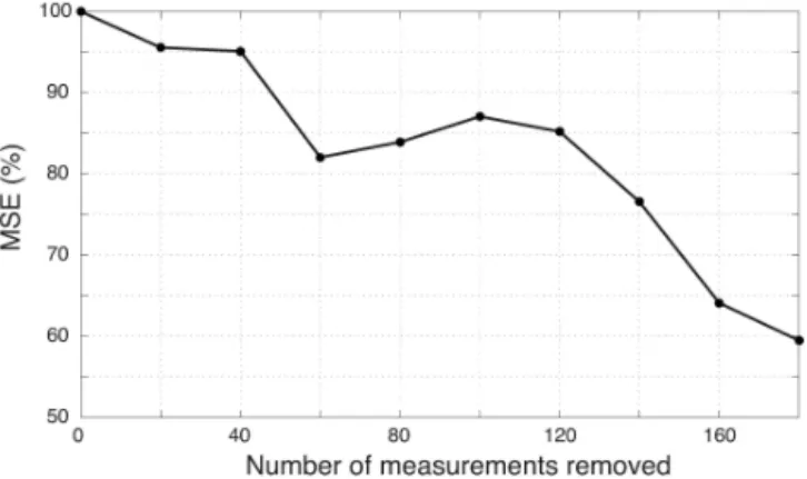
Imagine that we have an oracle which reveals to us the mea-surements corresponding to the largest errors (i.e., the out-liers). If we remove these measurements from the data set, the performance of Eq. (2), in terms of the reconstruction er-ror or mean square erer-ror (MSE), improves significantly.1In order to illustrate this, we remove the measurements asso-ciated with the largest errors (sorted by magnitude) and ob-serve the effect on the MSE. Figure 2 shows how the MSE decreases as more and more outliers are removed. Some os-cillations may occur due to outlier compensation effects.
1The MSE is defined as1
nkx− ˆxk22, wherexˆ is the estimated source,xis the real source (ground truth), andnis the number of elements inx.
Figure 2. MSE of reconstruction obtained using Eq. (2). The strongest outlier measurements (the ones associated with the largest errors) have been removed manually. Notice that the MSE decreases as more outliers are removed.
However, in a real-world problem, we do not have such an oracle. The question becomes thus: how could one locate the outliers blindly?
3.1 RANSAC
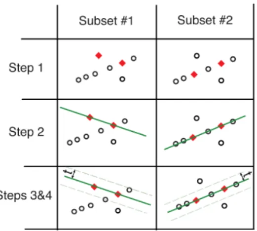
One of the simplest and most popular algorithms to local-ize outliers blindly is RANSAC. RANSAC has been widely and successfully used, mainly by the computer vision com-munity (Stewart, 1999). Figure 3 illustrates the operation of RANSAC, and algorithm 1 describes it in pseudocode.
Given a data setywithmmeasurements, select randomly
a subsety′containingp measurements. Typically,n < p < m, wheren is the number of unknowns in the problem. In
Fig. 3,m=8 andp=2, and the subset is shown in red dia-monds. Using Eq. (2) andy′, estimatexˆ, and then compute the residualr=Aˆx−y. Now, we can count how many of the original samples are “inliers”. For a given toleranceη, the set
of inliers is defined asL= {q∈ {1,2, . . . , m} |η≥(r[q])2}.
Repeat this processN times and declare the final solution
x∗to be that estimatexˆ which produced the most inliers. In Fig. 3,N=2.
Note that other regularizations can be used instead of Eq. (2). Here, we use the Tikhonov regularization because it is simple, general, and most other existing approaches are based on it. Nevertheless, if some properties of the source are known a priori (e.g., sparsity or smoothness), this step of the algorithm can be adapted accordingly.
A′←A[k,:] ˆ
x←arg min x
kA′x−y′k22+λkxk22
r←Axˆ−y
L← {q∈ {1,2,· · ·, m} |η≥(r[q])2} if#L>#L∗then
L∗←L x∗← ˆx end if end for return x∗
produces more inliers than the inferior solution (subset 1). Thus, RANSAC maximizes the number of inliers in the hope that this also minimizes the estimation error.
As we will see in the following sections, if the optimal value for the threshold parameterηis known and used,
us-ing RANSAC as a pre-processus-ing stage for outlier removal before applying Eq. (2) significantly improves the overall performance (compared to using only Eq. 2 with no outlier removal pre-processing). Unfortunately, the performance of RANSAC depends strongly on the parameterη, and finding
the optimal value ofηis an open problem.
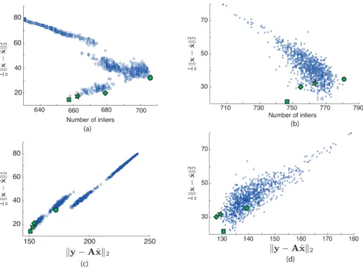
Furthermore, the assumed inverse proportionality between the number of inliers and the MSE does not always hold in the presence of “critical measurements”. This is the case in the ETEX data set, as we can see in Fig. 4a.
3.2 Critical measurements
We identify critical measurements as those which have the largest influence in the source-estimation process. A quanti-tative measure of this influence is the Cook’s distance (Cook, 1977). Figure 5 shows the Cook’s distance of the ETEX mea-surements. It is easy to observe the peak that identifies the critical measurements.
Let us consider again the ETEX data set, the set of N
solutions xˆ that RANSAC generates, and their correspond-ing residuals r. It is interesting to note that the solutionsxˆ with the most inliers (the superior solutions, according to RANSAC) have high residuals at exactly the critical mea-surements. This is shown in Fig. 6. In other words, by con-sidering the critical measurements as outliers, these solutions achieve more inliers.
Figure 3.Visual representation of the functioning of RANSAC. Subset 1 and 2 represent two RANSAC iterations. The subset of measurements selected by RANSAC in each iteration is represented by red diamonds. Subset 1 contains one outlier. Hence, the solution corresponding with this subset generates fewer inliers than subset 2, which is free of outliers.
RANSAC assumes that all the measurements have the same influence; it just wants to maximize the number of in-liers, and does not care about which exact measurements are the inliers. This is why it fails, in this case, and the inverse proportionality between the number of inliers and the MSE does not hold.
In summary, RANSAC operates reliably when all of the measurements are of similar importance, because the in-verse proportionality between MSE and the number of inliers holds. However, when critical measurements are present, this proportionality does not hold, and RANSAC fails.
3.3 RANdom SAmple Consensus (TRANSAC)
In order to avoid the weakness of the standard RANSAC algorithm, we propose an alternative indirect metric to discriminate solutions with small MSE: the total residual
ǫ = k Axˆ − yk2. By replacing the number of inliers by the total residual metric, we create the first step of the To-tal residual RANdom SAmple Consensus (TRANSAC) al-gorithm. The second step consists of a “voting” stage. Both are described in algorithm 2 in pseudocode.
The total residual is directly proportional to the MSE of re-construction. Unlike the number of inliers, this proportional-ity is also conserved when critical measurements are present in the data set (Fig. 4c and d). In a real-life problem, where we do not have access to the ground truth, we do not know if critical measurements are present. Hence, we need a robust algorithm like TRANSAC. In addition, TRANSAC does not depend on the thresholdη.
Figure 4.Performance of RANSAC and TRANSAC.(a)and(b)show graphically the correlation between MSE of reconstruction and the number of inliers.(c)and(d)show graphically the correlation between MSE of reconstruction and the total residual. To build(a)and(c) the complete data set was used, to build(b)and(d)the data set without critical measurements was used. The diamond indicates the solution obtained by the traditional Tikhonov regularization in Eq. (2), the star indicates the solution chosen by TRANSAC before the voting stage, the square indicates the final solution of TRANSAC, and the hexagon the solution chosen by RANSAC.
Figure 5.Cook’s distance of the measurements in the ETEX data set.
the candidate solutions with a total residual under a certain threshold, to come up with the best possible final solution.
Intuitively, the solutions with the smallest total residual (i.e., smallest MSE) are generated using almost outlier-free random subsets of measurements y′. We refer to these as the “good” subsets. Outliers can appear sporadicly in some of these good subsets, but the same outlier is extremely un-likely to appear in all of them. Hence, in the voting stage, we select the measurements that all the good subsets have in common, or, in other words, exclude any measurements that appear very infrequently.
Thus, we first select the subsets y′ associated with can-didate solutions with a total residual smaller than a certain threshold,ǫ < β. Then, for each measurement we count how
many times it appears in these good subsets. Finally, we se-lect the Mmeasurements with the largest frequency of
oc-currence.
4 Results
4.1 Performance analysis of TRANSAC
We now perform two experiments to demonstrate various as-pects of TRANSAC.
4.1.1 Sanity check
In Sect. 3.3, we confirmed the expected behavior of the first stage of TRANSAC: we showed that the total residual is di-rectly proportional to the MSE. Let us now check the second stage: the voting. To do so, let us suppose that, during the voting, we have access to the MSE of every candidate solu-tionxˆ. Then, we would of course select the solutions which, in fact, have the smallest MSE, and use them to build the his-togram. We run this modified TRANSAC with the data set without critical measurements.
Figure 7a shows the MSE obtained for different values of the parameterM. The dashed line on the right indicates
the maximum possible value ofM, such thatM=m, which
corresponds to using the whole measurement data set. The dashed line on the left indicates the minimum possible value,
M=n, and corresponds to using as many measurements as
k←punique random integers from[1, m] y′←y[k]
A′←A[k,:] ˆ
x←arg min x
kA′x−y′k22+λkxk22 ǫ[s] ←kAxˆ−yk2
K[ :, s] ←k end for
G← {q∈ {1,2,· · ·, N} |ǫ[q] ≤β} KG←K[:,G]
h[k] ←how many timeskappears inKG,∀k∈ {1,2,· · ·, m} b←indices of theMlargest elements ofh
y∗←y[b] A∗←A[b,:] x∗←arg min
x
kA∗x−y∗k22+λkxk22
return x∗
We can observe that the MSE of the solution increases as
Mincreases. This is to be expected: asMgrows, more
out-liers are included in the data set that is used to obtain x∗, and its MSE increases. We note that the result curve is non-decreasing, because, in this particular experiment, we have access to the MSE, and the histogramhis built from the ac-tual best-candidate solutions.
4.1.2 Actual ETEX
In this subsection, the performance of the complete TRANSAC algorithm is examined. Let us consider first the data set without critical measurements. As in the sanity check above, TRANSAC is run for different values ofM. The
re-sults are shown in Fig. 7b. We observe that the MSE increases as Mincreases, as before, and the maximum MSE still
oc-curs atM=m. This is reassuring: even if we do not find the
optimal value for the parameterM, we will improve the
solu-tion (with respect to using only the Tikhonov regularizasolu-tion) by taking anyn < M < m. Notice that the minimum MSE
occurs again whenM=n.
Figure 7c shows the results from the examination of the whole data set, including the critical measurements. We can observe that, again, the maximum MSE occurs atM=m. On
the other hand, the minimum MSE does not occur at n, but
rather atM=330. Also, although the exact performance of the algorithm varies with the value chosen for the parameter
Figure 6.Residuals of two different source estimations: The blue peaks correspond to the residual produced by the solutionxˆ with
the largest number of inliers in Fig. 4a. The black arrows on the top indicate where the two most critical measurements are localized. Clearly, the residual corresponding to these two measurements is much larger than the rest. The red peaks corresponds to the residual produced by the solutionxˆ with the smallest MSE in Fig. 4a.
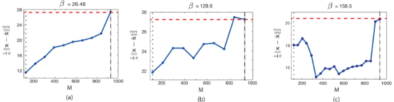
β, as shown in Fig. 8, we note that, for practically any value
ofβ, there is an improvement in performance.
These results show that TRANSAC clearly improves the performance of the Tikhonov regularization in both cases (with and without critical measurements).
4.2 Outlier removal
As explained in Sect. 3, RANSAC and TRANSAC are blind outlier-detection algorithms that can be combined with dif-ferent regularizations in order to improve their results. In this section we combine RANSAC and TRANSAC with two different regularizations previously used in the literature, Eqs. (2) and (3), and study their performance. As before, we use the ETEX data set with and without the critical measure-ments.
The results are shown in Fig. 9. It is important to note that all of these results were generated using the optimal values for all of the parameters (λ,η,β,M) that were found
Figure 7.Performance of TRANSAC combined with Tikhonov regularization. In the three plots, the red dashed line indicates the estimation error given by typical Tikhonov (Eq. 2). The dashed line on the right indicatesM=m, the one on the left indicatesM=n. Plot(a)shows the results of the sanity check. As the selected number of measurementsM increases, the MSE of the estimation decreases. Notice that the maximum MSE corresponds withM=m. Plot (b)shows the results of applying TRANSAC to the ETEX data set without critical measurements. Again, the MSE increases in general with M, and the maximum MSE appears in M=m. Plot (c)shows the results of applying TRANSAC to the whole ETEX data set, critical measurements included. In this case, the MSE does not always increase withM, but the maximum MSE still corresponds withM=m.
Figure 8.Sensibility of TRANSAC combined with Tikhonov regu-larization to the parameterβ. The red line indicates the estimation error given by typical Tikhonov (Eq. 2). The algorithm is sensitive to beta, but, for practically all beta values, the performance is im-proved.
that the MSE is higher, i.e., the reconstruction is poorer when the critical measurements are not used, which is, again, con-sistent with our analysis.
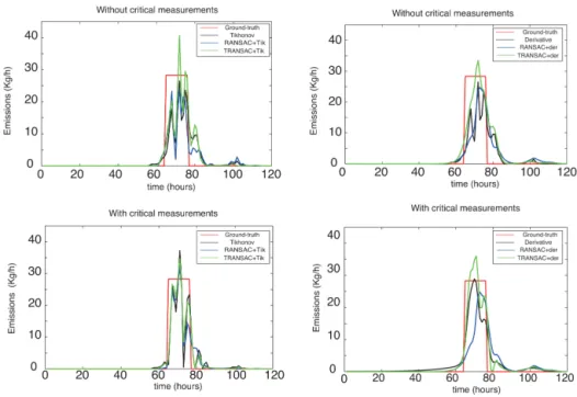
Figure 10 gives a more qualitative assessment of these re-sults by representing the estimated source. We first notice that the reconstructed sources using Eq. (3) are generally smoother than those reconstructed using Eq. (2), due to the added smoothness (derivative) term in the objective function. Next, we note that the reconstructions using the critical mea-surements are closer to the ground truth than the reconstruc-tions without the use of the critical measurements, which is consistent with the results shown in Fig. 9. Finally, we note that in all four cases, the recovered source using TRANSAC for the outlier detection produces the closest match to the ground truth, as expected.
Figure 9.MSE of source estimated by different algorithms. The blue bars correspond with the original algorithms (Eqs. 2, 3). The violet bars indicate that RANSAC is used for outlier removal, and the green ones shows that TRANSAC is used for outlier removal. The plot on the left was generated using the whole ETEX data set. The plot on the right was generated using the ETEX data set without critical measurements.
5 Conclusions
In this work we showed that the additive errors present in the ETEX data set come from a heavy-tailed distribution. This implies the presence of outliers. Existing source-estimation algorithms typically assume Gaussian additive errors. This assumption makes such existing algorithms highly sensitive to outliers. We showed that, if the outliers are removed from the data set, the estimation given by these algorithms im-proves substantially.
Figure 10.Source reconstructions given by the different algorithms. The plots on the left were generated combining Eq. (2) with RANSAC and TRANSAC. The plots on the right were generated combining Eq. (3) with TRANSAC and RANSAC. The plots on the top were generated using the ETEX data set without critical measurements. The plots on the bottom were generated using the whole ETEX data set.
to critical measurements. To overcome these difficulties, we created TRANSAC, a modification of RANSAC, which also includes a voting stage.
To demonstrate the efficiency of these methods in a real-world problem, we used the ETEX tracer experiment data set. The source was first recovered with two previously proposed source-estimation algorithms that assume Gaussian additive errors – Eqs. (2) and (3). Then, it was recovered again with our algorithms that use RANSAC and TRANSAC. The re-sults clearly display how the source estimation improves if an outlier-detection algorithm is used. They also show that the performance of our proposed algorithm TRANSAC clearly exceeds the performance of RANSAC in every case.
Acknowledgements. This work was supported by a Swiss National Science Foundation grant: Non-linear Sampling Methods, FNS-200021_138081.
Edited by: A. B. Guenther
References
Bocquet, M.: High-resolution reconstruction of a tracer dispersion event: application to ETEX, Q. J. Roy. Meteorol. Soc., 133, 1013–1026, 2007.
Cook, R. D.: Detection of Influential Observation in Linear Regres-sion, Technometrics, 19, 15–18, 1977.
CTBTO: Preparatory Commision for the Comprehensive Nuclear-Test-Ban Treaty Organization, available at: www.ctbto.org (last access: 8 October 2014), 2014.
Draxler, R., Dietz, R., Lagomarsino, R., and Start, G.: Across North America tracer experiment (ANATEX): Sampling and analysis, Atmos. Environ. A-Gen., 25, 2815–2836, 1991.
Fischler, M. A. and Bolles, R. C.: Random sample consensus: A paradigm for model fitting with applications to image analysis and automated cartography, Comm. ACM, 24, 381–395, 1981. Holmes, N. and Morawska, L.: A review of Dispersion Modelling
and its application to the dispersion of particles: An overview of different dispersion models available, Atmos. Environ., 40, 5902–5928, 2006.
Martinez-Camara, M., Dokmanic, I., Ranieri, J., Scheibler, R., Vet-terli, M., and Stohl, A.: The Fukushima Inverse Problem, in: 38th International Conference on Acoustics, Speech, and Signal Pro-cessing, 2013.
Nodop, K., Connolly, R., and Giraldi, F.: The field campaigns of the European Tracer Experiment (ETEX): overview and results, Atmos. Environ., 32, 4095–4108, 1998.
Rousseeuw, P. J. and Leroy, A. M.: Robust Regression and Outlier Detection, John Wiley & Sons, Inc., New York, NY, USA, 1987. Seibert, P.: Inverse modelling with a Lagrangian particle dispersion model: application to point releases over limited time intervals, Air Pollution Modeling and Its Application XI, 381–389, 2001. Stewart, C. V.: Robust Parameter Estimation in Computer Vision,
SIAM Rev., 41, 513–537, 1999.
Stohl, A., Hittenberger, M., and Wotawa, G.: Validation of the La-grangian particle dispersion model FLEXPART against large-scale tracer experiment data, Atmos. Environ., 32, 4245–4264, 1998.
Stohl, A., Seibert, P., Wotawa, G., Arnold, D., Burkhart, J. F., Eck-hardt, S., Tapia, C., Vargas, A., and Yasunari, T. J.: Xenon-133 and caesium-137 releases into the atmosphere from the Fukushima Dai-ichi nuclear power plant: determination of the source term, atmospheric dispersion, and deposition, Atmos. Chem. Phys., 12, 2313–2343, doi:10.5194/acp-12-2313-2012, 2012.
Winiarek, V., Bocquet, M., and Mathieu, O. S. A.: Estima-tions of errors in the inverse modeling of accidental release of atmospheric pollutant: Application to the reconstruction of the cesium-137 and iodine-131 source terms from the Fuk-shima Dai-ichi power plant, J. Geophys. Res., 117, D05122, doi:10.1029/2011JD016932, 2012.