What happens after the Central Bank of Brazil increases the target interbank rate by 1%?

(1)

• •

FUNDAÇÃO GETULIO VARGAS

ｾｾ＠

FGV

p/EPGE

EPGE

,

SEMINARIOS DE PESQUISA

ECONÔMICA DA EPGE

"What Happens After the Central 8ank of

Brazillncreases the'Target

Interbank Rate By 1

%?"

RUBENS PENHA CVSNE

(EPGE/FGV)

Data: 10/03/2005 (Quinta-feira)

Horário: 16 h

Local:

Praia de Botafogo, 190 - 110 _andar

Auditório nO 1

Coordenação:

(2)

,

Xi

What

Happens After the Central Bank of

Brazil Increases the Target Interbank

Rate

By

1%?*

Rubens Penha Cysne

t

March 8, 2005

Abstract

In this paper I use Taylor's (2001) model and Vector Auto Regres-sions to shed some light on the evolution of some key macroeconomic variables after the Central Bank of Brazil, through the COPOM, in-creases the target interest rate by 1%. From a quantitative perspec-tive, the best estimate from the empírical analysis, obtained with a 1994 : 2 - 2004 : 2 subsample of the data, is that GDP goes through an accumulated decline, over the next four years, around 0.08%. In-novations to interest rates explain around 9.2% of the forecast erro r of GDP.

1 Introduction

The current approach to monetary policy in Brazil is characterized by the setting of two different targets: the infiation target and the targeting of the rate at which financiaI institutions Iend each other reserves overnight (the interbank overnight interest rate target). Infiation targeting was introduced

*Work in progress, please do not quote. I am thankful to Lutz Kilian, for making available some of the computer codes used in this work. The usual disclaimer applies. Key Words: Inflation, Open-Mouth Operations, VAR, Vector Auto Regression, Bias-Corrected Bootstrap. CEL codes: C15, E40, E50.

(3)

..

in Brazil in July /1999. Once the policy of controlling the nominal exchange rate was abandoned by the Central Bank, at the beginning of 1999, a new forward-Iooking regime enhancing transparency and the control of expecta-tions emerged as the right thing to do.

The interbank-rate targeting is the main operational tooI by means of which infiation is kept equal or elose to its target. It amounts in practice to two coordinated policies conducted by the Central Bank. The first poIicy regards the announcements of the interest-rate trends and/or targets for the near future. It is a responsibility of the COPOM1 , which hoIds monthly meetings with this purpose. The second policy, a responsibility of the Central Banks's Trading Desk, amounts to making daily open-market operations, in such a way that supply and demand for reserves intersect at an interest rate equaI or elose to the desired target. There is no direct interference of the Central Bank, through its Trading Desk, on the interbank rates.

Comparatively to the American experience in indirectly controlling the interbank rate, even though operationally the two systems are alike, there is at least one important technical difference. The relatively high statutory reserve requirements in Brazil generate a more predictable demand for bank reserves and facilitates the operations to be performed by the Trading Desk. Other than the compulsory reserve requirements, the demand for reserves is generated by interbank payment fiows. As pointed out by Furfine (2000), it is reasonable to assume that payment fiows are positively correlated with the uncertainty in reserve balances. Therefore, by affecting the demand for reserves out of a precautionary motive, payment fiows can be expected to be correlated with the leveI of the daily federal-funds rate.

Since the target interest rate is a crucial tool for the day-by-day policies of the Central Bank, it is very important to know how changes in this rate affect other relevant macroeconomic variables such as GDP, employment and infiation.

Several very elaborate econometric works have been produced by the Cen-tral Bank of Brazil since the introduction of the Inflation-Targeting regime, in order to provide a technical background for the forecasts to be announced. Among them, Bogdanski et aI. (2000) concentrates on the dynamics involv-ing interest rates, prices and output. These authors have coneluded, usinvolv-ing structural models, that interest rate changes affect aggregate demand in a period of 3 to 6 months, output gap having an impact on inflation after 3 months. This makes a total around nine months between a policy action based on the interest rate and curbing inflation. Tabak (2003) has found

(4)

- - - ,

that, to a certain extent, market participants have been able to anticipate some policy actions taken by the COPOM.

The VAR literature using Brazilian monetary data is of a high technical leveI, but not very vasto Pastore (1995, 1997) investigated inflation persis-tence and the passiveness of money supply to the inflation rate. Fiorencio and Moreira (1999) used a variabIe-coeilicient VAR to assess the ef:fectiveness of monetary policy in dif:ferent periods. Rabanal and Schwartz (2001) used 1995-2000 data to investigate output and money response to interest-rate shocks. Minella (2001, 2003) used monthly data from 1975 to 2000 to in-vestigate the link between interest rates, money and output and to compare three distinct periods of the Brazilian economy.

This work intends to add to the Brazilian monetary literature in two respects. First, a solution to Taylor's model is presented as a tool in the understanding of the link between the target interest rate and the overnight interest rate. The main conclusion of this analysis i$ that the convergence of interest rates to the target interest rate (which takes some days) can be as-sumed to be practically instantaneous, under the assumptions of a quarterly time period and a four-year horizon, for reasonable values of the underlying parameters. This allows for an interpretation of changes in the target interest rate as shocks to interest rates2_.

In a second step, a Vector-Auto-Regression (VAR) analysis is carried out with the purpose of investigating the dynamics of some macroeconomic variables. More particularly, I will be interested in the qualitative ef:fects of a one percent raise of interest rates on prices, output and reserves and, from a quantitative perspective, on the accumulated ef:fects of such a measure on GDP, over a four-year horizon. As it is always the case in such analyses, all results are contingent on the assumption that the relevant sigma algebra on which econornic agents base their expectations is the one generated solely by the series used in the econometric estimations.

2 Taylor's Model and Its Solution

Taylor (2001) of:fers an easily readable mo deI in which supply and demand for bank reserves are written, respectively, as3 :

(1)

2By defining the time of the shock as that in which the news are released.

31 am using the term "bank reserves" as a shortening to "bank reserves held as deposits in the Central Bank". This corresponds to what Taylor (2001) calls "fed balances".

(5)

•

and

bt = -a(rt - "(EtTt+l)

+

êt, a

>

O, O

< "( <

1 (2)

The first equation says that the supply of bank reserves (b) is increased, at time (day) t, by (indirect) actions of the Desk, when the interest rate in period t - 1 is higher than the targeted interest rate (p) at period t - 1. The second equation translates the demand of reserves by the banks. This demand is positive when banks expect, conditionally on the information set available at date t, that interest rates, corrected for the parameter "(, wiII increase from one day to another.

In terms of the classification presented in Simonsen and Cysne (1995,

p. 656), this is a mixed system of stochastic difference equations, since there are autoregressive and forward looking components. By assuming that information is not lost over time, (2) and the law of iterated expectations lead to:

00

Et-lTt =

_2..

_a

L

"(j Et-1bt+j

+

lim i,n Et-1Tt+n

n ... oo

j=O

which shows how the value interest rates expected to prevail in the future affect the present interest rate.

Taylor (2001) does not explicitly solve the system of equations given by

(1) and (2).

This can be easily done, under perfect foresight, in the case of an au-tonomous system (Pt = P for all t). By writing:

A=[l

CI.-y

ｾｬＬ＠

-y

(7) and (8) read:

Zt+l = AZt

+

Cp (3)

The fixed point and the characteristic equation of (3) are, respectively,

(4)

and

f(>-.)

=

>-.2 _ 1

+ "(

>-.

+

a - (3

"( a"(

I will concentrate here only in the generic case in which the eigenvalues are real and distinct. In this case the eigenvectors generate JR2 and we can consider the inverse of the matrix formed by the eigenvectors of A. The

(6)

and e2 = (L ｡ＨｬＺＺＺＺｾ￀ｾＩＮ＠ By making P = (e1, e2) and defining Z = P-1z, we

have the system in iagonalized form:

Zt+1 = DZt

+

p-1Cp

where D is a diagonal matrix having in the diagonal the eigenvalues À1 and

À2 . The general solution reads

b

t

=

c1Ài and ft

=

ｃＲ￀ｾＬ＠ the hats over the

variables having the obvious meaning.

Assuming that the parameters of the model generate

I

À1

1<

1 and

I

À2

I>

1, the transversality condition (saddle-path solution) implies C2 = O. Using

( 4) we have , in terms of the original variables of the system (since z = P z):

!1

1 [

ｾ＠

1 + [

-0:(1 - "(}P

1

a(1-')'À2) p

which determines C1 as a function of bo. The general solution then reads:

bt - (bo - 0:("( - l)p )Ài

Tt -(bo - 0:("( - l)p)Ài

0:(1 - "(À_{1 )}

+

0:("( - l)p, t ｾ＠ O

+p,

t ｾ＠ 1

(5)

(6)

Equations (5) and (6) determine the evolution ofthe endogenous variables

b and T , under different values of the parameters 0:, !3 and "(, when there are

changes of the target interest rate p.

Taylor uses the parameter values "( = 0.9, o: = 0.3 and!3 = 0.1 to draw Figure 5 in his work. Figure 5 shows the evolution of interest rates when the target interest rate changes from O to 0.5. The economy is supposed, previously to period zero, and including period zero, to be in a steady state with p = T

=

O and b = bo = O (the fact that bo = O follows from equation

(8), since in the steady state Tt = EtTt+1).

Note from (5) and (6) that when "(

=

1, bt = bo

=

O for all t, even though

the interest rate immediately adjusts to its new level. In other words, there is no need of open market operations to change interest rates. This is what Thornton (1999) and Guthrie and Wright (2000) referred to as "Open Mouth Operations" .

Below I present some additional simulations of the solutions to (7) and (8) using parameter values other than those used by Taylor:

Insert Figure 1 lIere

(7)

rates and reserves to converge to the new steady states. Seeing the figures in Figure 1 as disposed like a 2x3 matrix, Figures 1x3 and 2x3 show the instantaneous adjustment of interest rates and the invariance of the total leveI of reserves when

r

= 1, the case described above as the "open mouth" case. Figure 2x2 corresponds exactly to Figure 5 in Taylor (2001).

3 Innovation Accounting

The previous section shows that, under reasonable assumptions regarding the parameters of the model, one can expect the overnight interest rate to converge to the new target announced by the monetary authorities in a period ranging from one to ten days. FIom this section onwards, our time period will be of one quarter and our horizon of analysis will take a total of four years. Since a ten-days period under this horizon is practically negligible, one can associate news of changes in the target rate with immediate shocks to interest rates.

U nder this reasoning, from now on my purpose will be using impulse-response and variance-decomposition analysis to study what happens to out-put, price leveI, and bank reserves, once interest rates are increased by one percentile point (a hundred basis points)4.

Initially, I derive qualitative considerations working with the whole sam-pIe period in which the macroeconomic variables under consideration are available on a quarterly basis: 1980: 1 - 2004 : 2. Later on in this section I will be interested on more accurate responses, from a quantitative per-spective, regarding the present (after-Real) low-infiation experience, of how shocks in interest rates affect the evolution of GDP. In this case only the

post-Real data sample (1994 : 2 - 2004 : 2) is used.

3.1 Confidence Bands: Bias-corrected Booststrap

As in Cysne (2004), here I use the confidence bands for the impulse-response functions based on Kilian's (1998) bias-corrected bootstrap method.

The application of the standard bootstrap procedures to auto-regressive models generates replicates which are necessarily biased, on account of the small-sample bias of the estimators of the parameters. In order to deal

with this problem, specifically regarding the confidence intervals for

impulse-4 For the effect of changes in the target rate on the term structure of interest rates, in

(8)

response functions constructed from VAR estimates, Kilian (1998) proposed correcting the bias prior to bootstrapping the estimate.

Monte Carlo studies carried out by this author (see p.222 in Kilian (1998)) show that the relative frequency at which the 95% confidence interval covers the true impulse response (in a modellike the one used here) can be as low as 50% when standard bootstrap methods are employed. The bias-corrected bootstrap, on the other hand, presents a frequency around 90-95%5. In the formulation used here, I employ Pope's (1990) closed-form solution to the bias of the estimators of the VAR. The theorem reads:

Theorem 1 (Pope (1990)): Let Ân be the least-squares estimator of A in

the m-dimensional AR(l): X t = _AXt-1

+

Zt, in which X t and Zt are mxl

and A is mxm, based on a sample of size n. Make:

where Ut = -'<t -

X

n ,

X

n the sample mean. Suppose that, for some c

>

O, E 11

Cn(O)-l

II1+õ

ｾｉ＠

. II

states for the operator norm) is bounded as n ｾ＠ 00

and that the innovations Zt are a marlingale di.fference sequence such that all moments of Zt up to and including the sixth, conditional on the past, are finite and have values independent of t. Let G denote the conditional covariance of Zt, and suppose that

II

A

II

<

1. Then, as n ｾ＠ 00, the bias

Bn = EÂn - A is of the form:

where b is g1:ven by:

Bn =

_!!..

+

O(n-3/ 2 )

n (7)

The sum is over eigenvalues of A, weighted by their multiplicities, and r(j) =

EXtX'ftj'

Proof. See Pope (1990) . •

The key point to note is that the bias for the bootstrap is re-estimated, and new coefficients are generated, in each re-sample of the bootstrap.

(9)

3.2 Impulse-Response Functions

Let y, p, r, res and m denote, respectively, the logaríthm of real GDP, the

logarithm of the price index, the short term (Selicti₎ _{interest rate, the}

loga-rithm of total (bank) reserves and the logaloga-rithm of M1 (means of payment).

The primitive data on p, m and r used here are from IBRE-FGV's7 data

bank. The quarterly GDP index and bank reserves are from IPEA8.

In all estimations in this work, the benchmark specification used,

regard-ing the orderregard-ing of the variables in the V AR, is the same as in Christiano et aI. (2000). Under this ordering, the information set assumed to be available to the government at time t, when choosing the ínterest rate to target, in-cludes the current and lagged values of y and p, as well as lagged values of r, res and m. As a consequence of the ordering of the variables in the VAR and of the Cholesky-orthogonalization assumption, neither the price leveI at time t nor the GDP at time t are supposed to change as a consequence of a contemporaneous interest-rate shock9 .

• Results For The Model in Log LeveIs

Since the main goal here is to determine the interrelationships among the variabIes, not the parameter estimates, in this subsection I follow Sims's

(1980) and Doan's (1992) suggestionslO _{and estimate the VAR in Iog leveIs.}

A preliminary anaIysis of this data set has been carried out by Cysne

(2004). Using the Akaike and the Schwarz criteriall , the model with 12 Iags

6 Selic is a shortening for "Sistema Especial de Liquidação e Custódia."

7Instituto Brasileiro de Economia da Fundação Getulio Vargas. 8Instituto de Pesquisa Econômica Aplicada.

9The fact that interest rates do not affect output contemporaneously can be justified by previous work of Bogdanski et ai (2000), who found, using structural models, that interest rate changes affect aggregate demand only after a period of 3 to 6 months.

lOSee also Enders (1995, p. 301).

11 The maximum estimated absolute value of the eigenvalues of the A.R. matrix for 4, 8

and 12 lags are, respectively, 0.9815, 0.9829 and 0.9930. Reestimations of the VAR over the same sample period lead to values of the Akaike Information Criterion, respectively, for the model with 4, 8 and 12 lags, of 1.0969 1.1392 and -0.7527. This suggests the use of the model with 12 lags. Even though we are dealing with a small sample, I also performed a log-likelihood test under a null of 12 lags and an alternative of 8 lags. Asymptotically,

c = 2

*

(L12 - L8) has a chi-square distribution with 100 (52_.4)_{degrees of freedom. The}

value found was 367.2, confirming the Akaike-Criterion option for 12 lags. Sims' (1980)

bias-corrected version ofthis test calls for multiplying this statistics by (nl -n2)/nl, where nl is the number of periods effectively used in the regressions and n2 is the number of

(10)

outperformed the models with 4 and 8 lags.

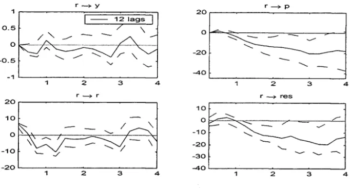
For these reasons, regarding the whole data sample, I shall work here only with 12 lags, The figures below show the response of output and prices to an increase of one standard deviation in interest rates, using a VAR in log leveIs with a nonzero intercept and 12 lags:

Insert Figure 2 Here

The four sub-figures in Figure 2 show the response of y, p, r and res to a

one percent increase in interest rates. As one can observe from the "r --+ y"

figure, the product declines in the first quarter to a maximum around 0.3% but recovers before the end of the year12_. _{There is a rebound after the end of}

the first year and a subsequent decline one quarter afterwards, which last for two years. A new rebound after the third year is then followed by a further decline. By aggregating the effects over the GDP over the whole four-year horizon one finds an accumulated product decline around 0.44%13.

As shown by Cysne (2004), there is a subtle price puzzle in the first quarter after interest rates are increased. As of this date, though, the effect of interests on prices is of a four-year persistent decline.

Regarding the interest rate itself, the shock lasts around one quarter. Finally, with respect to bank reserves, the contemporaneous effect is negative, with a rebound at the end of the first quarter that lasts for three quarters. After the end of the first year, the negative eífect of interest rates on reserves lasts for the next three years .

• Trends and Unit Roots

It is a valid exercise checking how the results obtained by running the VAR in log leveIs, without a trend, could change by using first differences of the nonstationary variables, or by the introduction of a time trend for the regressions run in log leveIs. The respective impulse-response functions are shown in Figures . The results in differences were obtained with four lags. To avoid clustering the analysis, I do not include confidence bands here.

12Considering on1y the initia1 cycle shown by GDP, this is in agreement with Lisboa (2004), who has argued that the short-run effect, on output and employment, of an increase of the target interest rate by the COPOM is temporary and 1asts 1ess than a year.

(11)

Insert Figure 3 and 4 Here

Regarding the estimation in log leveIs with a trend (the nonzero intercept is assumed in all cases), the overall shape of the responses of all variables is practically the same as in the case without trend. This could be expected, given the large number of regressors in each equation. A quantitative differ-ence is that now the overall decline of product along the four years is found to be 0.29%, a bit lower than the previous 0.44%.

Qualitatively, imposing unit root to the nonstationary variables Ieads to some changes in the shape of the responses, but not significant ones (Figure 4). GDP still declines just after the interest-rate shock and recovers by the end of the firs year. The three-peak format of figure 1 in now sharper, with a positive response by the second year.

The value of the accumuIated decline in GDP over the four years now amounts to 1.23%, much higher than the previous 0.44%, but still in the range delimited by the same type of calculation using the confidence bands (see footnote 13).

The price puzzle is a bit longer, lasting around six to nine months. But the overall response of prices is negative, repeating the previous resulto Re-garding interest rates, the shock lasts for around six months, as opposed to the previous three months. As before, bank reserves increase just after the shock, but fall around one year and a half afterwards.

3.3 Variance Decomposition

The purpose of this subsection is to measure the proportion of movements in each of the sequences considered that can be attributed to its own shocks, or to shocks to other variables. The same assumptions regarding the ordering of the variables in the VAR used to obtain the impulse-response functions apply here. The horizon considered is of four years. I provide variance decomposition for the model in log leveIs only.

The results displayed in Figure 5 show that interest rates explain a re1-ative1y small share of the conditiona1 variance of GDP (4.9%). Regarding prices, interest rates, bank reserves and money, though, the effect of shocks to interest rates in exp1aining forecast errors is usually very relevant. Unex-pected movements in interest rates account for around 39% of the variance of prices, 35% of the variance of bank reserves and 36% of the variance of MI . Except for the effect on GDP, shocks to interest rates play a more important

(12)

role in explaining forecast errors than shocks to money. Price and interest-rate shocks, alone, explain around 80% of the forecast errors in reserves and money.

4 Subsampling: Results For The Post-Real

Economy

The results obtained so far are satisfactory from a qualitative perspective but are not ideal for a description of the economy àfter the Real Plano The main reason is that as of 1994 : 2, macroeconomic variables evolved under a very different pattern. For instance, considering the whole sample, from

1980 : 1 to 2004 : 2, the standard deviation of the residuaIs in the estimation of y, p, r, re:s and m, conditional on a sigma algebra generated by the last four lags of each variable, were equal to around, respectively14, 2%, 12%, 31.45%, 17% and 8%. For the period 1994:2 - 2004:2, these values decline to, respectively, 0.68%, 1.14%, 0.35%, 11.48% and 3.26%.

The high variance of the residuaIs of the equation determining interest rates, for instance, explain the intercept around 6.6% in the contemporane-ous effect in interest rates of a 1% increase in r in Figure 2. This is very far, quantitatively, from what one would expect in the after- Real period.

This suggest that, if we want a reasonable quantitative answer regarding the accumulated GDP loss after the Central Bank of Brazil raises the target rate, we should resample the data to include only the 1994:2 - 2004:2 period. Since we are using quarterly data (there are no monthly estimates of GDP in Brazil), this leaves us with too little degrees of freedom to consider more than four lags. The product and interest-rate response are as expected, and are shown below:

The new estimations lead to a contemporaneous effect on interest rates of only around 0.34% and to an accumulated interest rate increase, over the four-year horizon, of 0.16%. Regarding the GDP, the new accumulated product loss is 0.08%. Using the lower and upper bands lead to a GDP variation of -1.24% and 1.31%. Note that this interval is contained in the

(13)

[-1.47%,1.31%] previously calculated for the whole sample. The new esti-mate of 0.08% accumulated GDP loss, though, as opposed to the old one of

0.44%, fits better the Post-Real economy.

The new variance decomposition for the subsample 1994:2-2004:2 is pre-sented in Figure 7.

The results displayed in Figure 7 show that interest rates in the more recent period explain a larger share of the conditional variance of GDP (9.2%,

as opposed to the previous 4.9%). Unexpected movements in interest rates now account for 2.14% of the variance of prices, 20% of the variance of bank reserves and 6% of the variance of MI . Shocks to money are now more

important than shocks to interest rates in explaining errors in the forecast of all variables, except interest rates themselves.

5 Conclusions

In this work we have started with a short description of the two-target

mech-anism that characterizes the present state of monetary policy in Brazil. Next, we solved and simulated Taylor's model for the determination of interbank interest rates. We have also seen that some parameter values of Taylor's modellead to what is generally called "" open-mouth" operations, as opposed to "open-market" operations.

In the second part of the paper, we have provided a VAR analysis of the

effects of increases in the target interest rate in the dynamic evolution of GDP, prices, interest rates and bank reserves. Our main findings have been that, qualitatively, prices and GDP fall after interest rates are increased, and that this behavior is robust to imposing unit roots on some variables and to including a trend in the regressions run in log leveIs.

From a quantitative perspective, we have found that in the Post-Real economy a one percent increase in interest rates lead to a accumulated prod-uct decline over the next four years around 0.08%, and that interest-rate shocks explain around 9.2% of the conditional variance of GDP.

References

(14)

[2] Christiano, Lawrence, Martin Eichenbaum and Charles Evans, 2000, "Monetary policy shocks: what have we learned and to what end?" In

MichaeI Woodford and John Taylor, eds., Handbook of Macroeconomics N orth Holland.

[3] Cysne, R. P., 2004, Is There a Price Puzzle in Brazil? An Application of Bias-Corrected Bootstrap. Ensaio Economico da EPGE n. 577. [4] Doan, Thomas A., 1992, RATS User's Manual, Evanston, IH. Estima. [5] Enders, W., 1995, Applied Econometric Time Series, Wiley Series in

ProbabHity and Mathematical Statistics, New York, USA.

[6] Fiorencio, Antonio, and Ajax R. B. Moreira (1999), "Latent Indexation and Ex,:::hange Rate Passthrough", Rio de Janeiro, IPEA, Texto para Discussào no. 650, Jun.

[7] Furfine, C. H., -(2000), Interbank payments and the daily federal funds rates. Journal of Monetary Economics 46:535-553.

[8] Guthrie, G. and Wright, J., 2000, "Open mouth operations", Journal of Monetary Economics 46 (2000) 489}516.

[9] Kilian, L., 1998, Small-Sample Confidence Intervals for Impulse-Response Functions. The Review of Economics and Statistics, 80, 218-230.

[10] Lisboa, M. 2004, Interview, Jornal Folha de São Paulo, 23/10/2004, Page B-4.

[11] Minella, A., (2001), Monetary Policy and Inflation in Brazil (1975-2000): a VAR Estimation, Working Paper Series 33, Central Bank of Brazil. [12] Minella, A., (2003), Monetary Policy and Infiation in Brazil (1975-2000):

a VAR Estimation, Rev. Bras. Econ. voI.57 no.3 Rio de Janeiro.

[13] Pastore, Affonso C. (1995), "Déficit Público, a Sustentabilidade do Crescimento das Dívidas Interna e Externa, Senhoriagem e In:j:ação: uma Análise do Regime Monetário Brasileiro", Revista de Econometria, voI. 14, no. 2, pp. 177-234.

(15)

[15] Pope, Alun L., 1990, Biases of Estimators in Multivariate Non-Gaussian Autoregressions. Journal of Time Series Analysis 11, 249-258.

[16] Rabanal, Pau, and Gerd Schwartz (2001), "Testing the ｅｾｬ･｣ｴｩｶ･ｮ･ｳｳ＠

of the Overnight Interest Rate as a Monetary Policy Instrument", In: International Monetary Fund, Brazil: selected issues and statistical ap-pendix, IMF Country Report No. 01/10, Washington, D.C., Jan. [17] Simonsen, M. H. and eysne, Rubens P. (1995): "Macroeconomia,

Sec-ond Edition". Editora Atlas, São Paulo.

[18] Sims, Christopher A., 1980, Macroeconomics and Reality, Econometrica, 48:1-48.

[19] Tabak, B. M., 2003 Monetary Policy Surprises and the Brazilian Term Structure of Interest Rates, Working Paper Series n. 30, Central Bank of Brazil

[20] Taylor, J. 2001, Expectations, Open Market Operations, and Changes in the Federal Funds Rate. Federal Reserve Bank of St. Louis.

(16)

ｲｨｯｾ＠ b

o o 1

-- gamma=.5 -- gamma=.9

1-

gamma=1

-0.02 0.5

0.005

..o -0.04 O

-0.01

-0.06 -0.5

-0.08 0.015 -1

O 5 10 O 5 10 O 5 10

t rho ｾ＠ r

0.5 0.5 0.5

I

0.4 0.4 0.4

0.3 0.3 0.3

0.2 0.2 0.2

0.1 0.1 0.1

O O

5 10 O 5 10 O 5 10

Figure 1: Response of Reserves and Interest Rates to a Unanticipated 0.5%

(17)

ｲｾｹ＠ｲｾｰ＠

1 20

1-

121ags

0.5 7 _\ _o _ｾ＠

/ " .-/

-

..;:::::

---'--....

-20 _'--

--0.5 _v "-

-'-- '--....

-1 -40

---1 2 3 4 1 2 3 4

r ｾ＠ r r ｾ＠ res

20

10

10 _O

----../'

O -10 '--....

-20

----

'--10

_----

'---30

-20 -40

1 2 3 4 1 2 3 4

Figure 2: ImpuIse-Response F\mctions, VAR in LeveIs Without a Trend

ｲｾｹ＠ｲｾ＠ p

1 20

121ags

0.5 _o

o

-20 -0.5

-40 -1

1 2 3 4 1 2 3 4

ｲｾ＠ r ｲｾ＠ res

20

10

10 _O ｾ＠

O -10

ｾ＠

-20 -10

-30

-20 -40

1 2 3 4 1 2 3 4

(18)

r -+ y r -+ p

20

0.5

1-

41ags

O

-20

-40 -1

2 3 4 1 2 3 4

r -+ r r -+ res

20

10

10 O

-10 O

-20

-10 -30

-40 -20

1 2 3 4 2 3 4

Figure 4: Impulse-Response Functions, VAR in First Differences

percentages af Farecast Errar variances in ROws Explained by calumns

y p r res m

y 54.08730 11.70066 4.90401 14.50732 14.80071 P 2.43134 42.82727 38.62835 1.64687 14.46617

r 7.30486 25.89850 29.272 54 9.77499 27.74911

res 5.56446 42.34591 35.69846 4.44005 11. 95111 m 4.40031 45.37274 36.28659 1.10138 12.83899

(19)

ｲｾ＠ y

0.8 0.6

I - 41a95. 1994-2004

0.6 0.5

"

1\

./ _\.1

/ \ 0.4

0.4 _\

r ../ _0.3

0.2

I \. 0.2

--

----o 0.1 /

/' _o

-0.2 _-./ _\

, / '

"- / -0.1

-004

-0.2

-0.6 _-0.3

..--'

.-,.

I

"-"- /'

-0.8 -0.4

1 2 3 4 1 2 3 4

Figure 6: Response GDP and Interest-Rate Response to a 1 % Increase of the Target Interest Rate, Subsample 1994:2-2004:2

y p r res m y 46.13374 12.68885 6.72749 8.23052 18.65238 P 10.91058 41.16261 8.14970 11. 24385 22.99661 r 9.16962 2.14983 46.39913 19.88458 6.22818 res 17.78556 14.14951 23.07689 34.12436 16.92237 m 16.00050 29.84920 15.64679 26.51669 35.20046

(20)

;. • 4 li f •

FUNDAÇÃO GETULIO VARGAS

BIBLIOTECA

lESTE VOLUME DEVE SER DEVOLVIDO A BIBLIOTECA NA ÚLTIMA DATA MARCADA

N.Cham. P/EPGE SPE C997w

Autor: Cysne, Rubens Penha

Título: What happens after the Central Bank ofBrazil

111111111111111111111111111111111111 111111111111111111