Submitted14 April 2016 Accepted 20 June 2016 Published20 July 2016 Corresponding author
Jeffrey M. Dick, [email protected]
Academic editor Vladimir Uversky
Additional Information and Declarations can be found on page 29
DOI10.7717/peerj.2238
Copyright 2016 Dick
Distributed under
Creative Commons CC-BY 4.0 OPEN ACCESS
Proteomic indicators of oxidation and
hydration state in colorectal cancer
Jeffrey M. Dick
Wattanothaipayap School, Chiang Mai, Thailand
ABSTRACT
New integrative approaches are needed to harness the potential of rapidly growing datasets of protein expression and microbial community composition in colorectal cancer. Chemical and thermodynamic models offer theoretical tools to describe populations of biomacromolecules and their relative potential for formation in different
microenvironmental conditions. The average oxidation state of carbon (ZC) can be
calculated as an elemental ratio from the chemical formulas of proteins, and water
demand per residue (nH2O) is computed by writing the overall formation reactions
of proteins from basis species. Using results reported in proteomic studies of clinical
samples, many datasets exhibit higher meanZC ornH2Oof proteins in carcinoma or
adenoma compared to normal tissue. In contrast, average protein compositions in
bacterial genomes often have lower ZC for bacteria enriched in fecal samples from
cancer patients compared to healthy donors. In thermodynamic calculations, the potential for formation of the cancer-related proteins is energetically favored by changes
in the chemical activity of H2O and fugacity of O2 that reflect the compositional
differences. The compositional analysis suggests that a systematic change in chemical composition is an essential feature of cancer proteomes, and the thermodynamic descriptions show that the observed proteomic transformations in host tissue could be promoted by relatively high microenvironmental oxidation and hydration states.
SubjectsBiochemistry, Mathematical Biology, Oncology
Keywords Colorectal cancer, Proteomics, Gut microbiome, Thermodynamics, Chemical components, Redox potential, Water activity
INTRODUCTION
Datasets for differentially expressed proteins in cancer are often interpreted from a mechanistic perspective that emphasizes molecular interactions. Alternative approaches exemplified by recent models that use information theory demonstrate the possibility of
interpreting proteomic expression data in a high-level conceptual framework (Rietman et
al.,2016). These approaches may combine concepts from dynamical systems theory and
thermodynamics, such as the possible association of ‘‘attractor states’’ in landscape models
with low-energy states of a system (Enver et al.,2009;Davies, Demetrius & Tuszynski,2011).
The purpose of the present study is to explore human proteomic and microbial community data for colorectal cancer within a chemical and thermodynamic framework using variables that represent oxidation and hydration state. This is carried out first by comparing chemical compositions of up- and down-expressed proteins along the normal tissue–adenoma–carcinoma progression. Then, a thermodynamic model is used to quantify the overall energetics of the proteomic transformations in terms of chemical potential variables. This approach reveals not only common patterns of chemical changes among many proteomic datasets, but also the possibility that proteomic transformations may be shaped by energetic constraints associated with the changing tumor microenvironment.
Recent years have seen the appearance of many proteomic datasets for colorectal cancer (CRC), a very common and extensively studied type of human cancer. Genomic
instability is often considered to be the primary driver of cancer progression (Kinzler &
Vogelstein,1996). However, not only genetic transformations, but also microenvironmental
dynamics can influence cancer progression (Schedin & Elias,2004). Many reactions in the
microenvironment, such as those involving hormones or cell–cell signaling interactions, operate on fast timescales, but local hypoxia in tumors and other microenvironmental changes can develop and persist over longer timescales. The long timescales of carcinogenesis may be sufficient for cells to adapt their proteomes to the differential energetic costs of biomolecular synthesis imposed by changing chemical conditions of the microenvironment.
One of the characteristic features of tumors is varying degrees of hypoxia (Höckel &
Vaupel,2001). Hypoxic conditions promote activation of hypoxia-inducible genes by the HIF-1 transcription factor and intensify the mitochondrial generation of reactive
oxygen species (ROS) (Murphy,2009), leading to oxidative stress (Höckel & Vaupel,2001;
Semenza,2008). It is important to note that there is significant intra-tumor and inter-tumor
heterogeneity of oxygenation levels (Höckel & Vaupel,2001;DeBerardinis & Cheng,2010).
Cancer cells can also exhibit changes in oxidation–reduction (redox) state; for example,
redox potential (Eh) monitoredin vivoin a fibrosarcoma cell line is altered compared to
normal fibroblasts (Hutter, Till & Greene,1997).
The hydration states of cancer cells and tissues may also vary considerably from their healthy counterparts. Microwave detection of differences in dielectric constant resulting from greater water content in malignant tissue is being developed for medical imaging of
breast cancer (Grzegorczyk et al.,2012). IR and Raman spectroscopic techniques also reveal
a greater hydration state of cancerous breast tissue, resulting from interaction of water molecules with hydrophilic cellular structures of cancer cells but negligible association with the triglycerides and other hydrophobic molecules that are more common in normal
tissue (Abramczyk et al.,2014).
Increased hydration levels may be associated with a higher abundance of hyaluronan
found in the extracellular matrix (ECM) of migrating and metastatic cells (Toole,
2002), while a higher subcellular hydration state may alter cell function by acting as a
signal for protein synthesis and cell proliferation (Häussinger,1996). It has also been
hypothesized that the increased hydration of cancer cells underlies a reversion to a more
thermodynamic variables related to redox and hydration state have been selected as the primary descriptive variables in this study.
As noted by others, it seems paradoxical that hypoxia, i.e., low oxygen partial pressure, could be a driving force for the generation of oxidative molecules. Possibly,
the mitochondrial generation of ROS is a cellular mechanism for oxygen sensing (Guzy
& Schumacker, 2006). Whether through hypoxia-induced oxidative stress or other mechanisms, proteins in cancer have been found to have a variety of oxidative post-translational modifications (PTM), including carbonylation and oxidation of cysteine
residues (Yeh et al.,2010;Yang et al., 2013). Although proteome-level assessments of
oxidative PTM are gaining traction (Yang et al., 2013), existing large-scale proteomic
datasets may carry other signals of oxidation state. One possible ‘‘syn-translational’’ indicator of oxidation state, inherent in the amino acid sequences of proteins, is the average oxidation state of carbon, which is introduced below. At the outset, it is not clear whether such a metric of oxidation state would more closely track hypoxia (i.e., relatively reducing conditions) that may arise in tumors, or a more oxidizing potential connected with ROS and oxidative PTM.
Density functional theory and other computational methods that yield electron density maps of proteins with known structure can be used to compute the partial charges, or oxidation states, of all the atoms. Spectroscopic methods can also be used to determine
oxidation states of atoms in molecules (Gupta et al.,2014). These theoretical and empirical
approaches offer the greatest precision in an oxidation state calculation, but it is difficult to apply them to the hundreds of proteins, many with undetermined three-dimensional structures, found to have significantly altered expression in proteomic experiments. Other methods for estimating the oxidation states of atoms in molecules may be needed to assess the overall direction of electron flow in a proteomic transformation.
Some textbooks of organic chemistry present the concept of formal oxidation states, in which the electron pair in a covalent bond is formally assigned to the more electronegative of
the two atoms (e.g.,Hendrickson, Cram & Hammond,1970, ch. 18). This rule is consistent
with the current IUPAC recommendations for calculating oxidation state of atoms in molecules, but generalizes the IUPAC definitions such that the oxidation states of different
carbon atoms in organic molecules can be distinguished (e.g.,Loock,2011;Gupta et al.,
2014). In the primary structure of a protein, where no metal atoms are present and
heteroatoms are bonded only to carbon and/or hydrogen, the average oxidation state of
carbon (ZC) can be calculated as an elemental ratio, which is easily obtained from the amino
acid composition (Dick,2014). In a protein with the chemical formula CcHhNnOoSs, the
average oxidation state of carbon (ZC) is
ZC=
3n+2o+2s−h
c . (1)
This equation is equivalent to others, also written in terms of numbers of the elements C,
H, N, O and S, used for the average oxidation state of carbon in algal biomass (Bohutskyi
et al.,2015), in humic and fulvic acids (Fekete et al.,2012), and for the nominal oxidation
Comparing the average carbon oxidation states in organic molecules is useful for
quantifying the reactions of complex mixtures of organic matter in aerosols (Kroll et al.,
2011), the growth of biomass (Hansen et al.,1994) and the production of biofuels (Borak,
Ort & Burbaum,2013;Bohutskyi et al.,2015). There is a considerable range of the average
oxidation state of carbon in different amino acids (Masiello et al.,2008;Amend et al.,
2013), with consequences for the energetics of synthesis depending on environmental
conditions (Amend & Shock,1998). Similarly, the nominal oxidation state of carbon can be
used as a proxy for the standard Gibbs energies of oxidation reactions of various organic
and biochemical molecules (Arndt et al.,2013). The oxidation state concept can be used
as a bookkeeping tool to understand electron flow in metabolic pathways, yet may receive
limited coverage in biochemistry courses (Halkides,2000). There has been scant attention
in the literature to the differences in carbon oxidation state among proteins or other
biomacromolecules. Nevertheless, the ease of computation makesZCa useful metric for
rapidly ascertaining the direction and magnitude of electron flow associated with proteomic transformations during disease progression.
Comparisons of oxidation states of carbon can be used to rank the energetics of reactions
of organic molecules in particular systems (Amend et al.,2013). However, quantifying the
energetics and mass-balance requirements of chemical transformations requires a more complete thermodynamic model. Thermodynamic models that are based on chemical components (or basis species), i.e., a minimum number of independent chemical formula units that can be combined to form any chemical species in the system, have an established
position in geochemistry (Anderson,2005;Bethke,2008). The implications of choosing
different sets of components, called the ‘‘basis’’ (Bethke,2008), have received relatively
little discussion in biochemistry, althoughAlberty(2004) in a similar context highlighted
the observation made byCallen(1985) that ‘‘[t]he choice of variables in terms of which a
given system is formulated, while seemingly an innocuous step, is often the most crucial step in the solution’’. Models built with different choices of components nevertheless yield
equivalent results when consistently parameterized (Morel & Hering,1993;Ravi Kanth et
al.,2014). Accordingly, components are a type of chemical accounting for reactions in a
system (Morel & Hering,1993), and do not necessarily constitute mechanistic models for
those reactions.
The structure and dynamics of the hydration shells of proteins have important biological
consequences (Levy & Onuchic,2006) and can be investigated in molecular simulation
studies (Wedberg, Abildskov & Peters,2012). Statistical thermodynamics can be used to
assess the effects of preferential hydration of protein surfaces on unfolding or other
conformational changes (Lazaridis & Karplus,2003). However, there is also a role for
H2O as a chemical component in stoichiometric reactions representing the mass-balance
requirements for formation of proteins with different amino acid sequences.
For example, a system of proteins composed of C, H, N, O and S can be described
using the (non-innocuous) components CO2, NH3, H2S, O2 and H2O. Accordingly,
stoichiometric reactions representing the formation of certain proteins at the expense of
and the other components. These stoichiometric reactions can be written without specific
knowledge of electron density in proteins or hydration by molecular H2O.
It bears repeating that reactions written using chemical components are not mechanistic representations. Instead, these reactions are specific statements of the requirement for mass balance that can be used to build thermodynamic models of chemically reacting
systems (Helgeson et al., 2009). Flux-balance models of metabolic networks integrate
stoichiometric constraints (e.g.,Hiller & Metallo,2013), but stoichiometric descriptions
of proteomic transformations are less common, perhaps because of a greater degree of abstraction away from elementary reactions. Nevertheless, the differentially down- and up-expressed proteins in a proteomic dataset furnish a quantitative description of a proteomic transformation and can be viewed as the initial and final states of a chemically reacting system, which is then amenable to thermodynamic modeling.
The chemical potentials of components can be used to describe the internal state of a system and, for an open system, its relation to the environment. Oxygen fugacity is
a variable that is related to the chemical potential of O2; it does not necessarily reflect
the concentration of O2, but instead indicates the distribution of species with different
oxidation states (Albarède,2011). Theoretical calculation of the energetics of reactions
as a function of oxygen fugacity provides a useful reference for the relative stabilities of
organic molecules in different environments (Helgeson et al.,2009;Amend et al.,2013).
However, in a cellular context a multidimensional approach may be required to quantify possible microenvironmental influences on the potentials for biochemical transformations. Likely variables include not only oxidation state but also water activity. Scenarios for early
metabolic and cellular evolution (Pace,1991;Russell & Hall,1997;Damer & Deamer,2015)
lend additional support to the choice of water activity as a primary variable of interest. A thermodynamic model that is formulated in terms of carefully selected basis species affords a convenient description of a system. As described in the Methods, a basis is selected that reduces the empirical correlation between average oxidation state of carbon
and the coefficient on H2O in formation reactions of proteins from basis species. The
first part of the Results shows compositional comparisons for human and microbial proteins (‘Compositional comparisons of human proteins’–‘Compositional comparisons of microbial proteins’) in 35 datasets from 20 different studies. Many of the comparisons
reveal higherZCor higher water demand for the formation of proteins up-expressed in
cancer compared to normal tissue. Contrary to the trends observed for human proteins,
the average protein compositions of bacteria enriched in cancer tend to have lowerZC.
METHODS
Data sourcesThis section describes the data sources and additional data processing steps applied in this study. An attempt was made to locate all currently available proteomic studies for clinical tissue on CRC including, among others, those listed in the ‘‘Tissue’’ and ‘‘Tissue
subproteomes’’ sections of the review paper byDe Wit et al. (2013) and in Supporting
Table 3 (‘‘Clinical Samples’’) of the review paper byMartínez-Aguilar et al.(2013). To
make the comparisons more robust, only datasets with at least 30 proteins in each of the up- and down-regulated groups were considered; however, all datasets from a given study were included if at least one of the datasets met this criterion. The reference keys for the
selected studies shown below and inTable 1are derived from the names of the authors and
year of publication.
In comparisons between groups of up- and down-expressed proteins, the convention in this study is to consider proteins with higher expression in normal tissue or less-advanced
cancer stages as a ‘‘normal’’ group (group 1), with number of proteinsn1, while proteins
with higher expression in cancer or more-advanced cancer stages are categorized as a
‘‘cancer’’ group (group 2), with number of proteins n2. For example, in the dataset
ofUzozie et al.(2014) comparing normal mucosa and adenoma, the proteins up-expressed
in adenoma are assigned to group 2, while in the adenoma—carcinoma dataset ofKnol et al.
(2014), the proteins with higher expression in adenoma are assigned to group 1 (seeTable 1).
Names or IDs of genes or proteins given in the sources were searched in UniProt (The
UniProt Consortium,2015). The corresponding UniProt IDs are provided in the*.csvdata
files inDataset S1. Amino acid sequences of human proteins were taken from the UniProt
reference proteome (filesUP000005640_9606.fasta.gzcontaining canonical, manually
reviewed sequences, andUP000005640_9606_additional.fasta.gzcontaining isoforms
and unreviewed sequences, dated 2016-04-13, downloaded from ftp://ftp.uniprot.org/
pub/databases/uniprot/current_release/knowledgebase/reference_proteomes/Eukaryota/). Entire sequences were used; i.e., signal peptides and propeptides were not removed when calculating the amino acid compositions. However, amino acid compositions were
calculated for particular isoforms, if these were identified in the sources. Fileshuman.aa.csv
andhuman_additional.aa.csvinDataset S1contain the amino acid compositions of the proteins calculated from the UniProt reference proteome. In a few cases, amino acid compositions of unreviewed or obsolete sequences in UniProt, not available in the
reference proteome, were individually compiled; these are contained in filehuman2.aa.csv
inDataset S1.
Reported gene names were converted to UniProt IDs using the UniProt mapping
tool (http://www.uniprot.org/mapping), and IPI accession numbers were converted to
UniProt IDs using the DAVID conversion tool (https://david.ncifcrf.gov/content.jsp?file=
Table 1 Summary of compositional comparisons for human proteins.Mean differences (MD), percent values of common language effect size (ES), andp-values are shown for comparisons between groups of proteins reported to have higher abundance in normal (n1) or cancer (n2) tissue (or less advanced or more advanced cancer stages, respectively). The textual descriptions are written such that the ordering around the slash (‘‘/’’) corresponds ton2/n1. References and specific abbreviations used in the descriptions are given in ‘Data sources’.
Reference (Description) n1 n2 ZC ¯nH2O
MD ES p-value MD ES p-value
WTK+08(T/N) 57 70 0.018 55 3e–01 0.006 52 7e–01
AKP+10(CRC nuclear matrix C/A) 101 28 −0.012 47 7e–01 −0.009 48 8e–01
AKP+10(CIN nuclear matrix C/A) 87 81 −0.031 40 3e–02 0.006 48 7e–01
AKP+10(MIN nuclear matrix C/A) 157 76 −0.002 52 7e–01 −0.013 45 3e–01
JKMF10(serum biomarkers up/down) 43 56 −0.007 46 5e–01 0.056 67 4e–03
XZC+10(stage I/normal) 48 166 0.009 52 7e–01 0.026 56 2e–01
XZC+10(stage II/normal) 77 321 0.022 60 6e–03 0.018 54 3e–01
ZYS+10(microdissected T/N) 60 57 0.019 58 1e–01 0.022 58 1e–01
BPV+11(adenoma/normal) 71 92 −0.023 40 4e–02 0.004 49 8e–01
BPV+11(stage I/normal) 109 72 -0.007 47 5e–01 0.005 50 9e–01
BPV+11(stage II/normal) 164 140 0.031 62 3e–04 0.006 51 7e–01
BPV+11(stage III/normal) 63 131 0.025 62 9e–03 −0.005 47 5e–01
BPV+11(stage IV/normal) 42 26 −0.010 44 4e–01 0.005 52 8e–01
JCF+11(T/N) 72 45 0.032 63 2e–02 −0.003 49 8e–01
MRK+11(adenoma/normal) 335 288 0.011 54 1e–01 0.058 68 2e–15
MRK+11(adenocarcinoma/adenoma) 373 257 0.034 65 1e–10 −0.009 47 1e–01
MRK+11(adenocarcinoma/normal) 351 232 0.034 63 4e–08 0.035 61 8e–06
KKL+12(poor/good prognosis) 75 61 0.026 64 5e–03 −0.002 48 8e–01
KYK+12(MSS-type T/N) 73 175 0.024 61 9e–03 0.023 56 1e–01
WOD+12(T/N) 79 677 0.016 54 2e–01 0.027 58 2e–02
YLZ+12(conditioned media T/N) 55 68 0.024 61 4e–02 0.009 54 5e–01
MCZ+13(stromal T/N) 33 37 0.047 74 5e–04 −0.034 42 2e–01
KWA+14(chromatin-binding C/A) 51 55 −0.039 29 2e–04 −0.010 48 7e–01
UNS+14(epithelial adenoma/normal) 58 65 0.001 49 8e–01 0.032 61 4e–02
WKP+14(tissue secretome T/N) 44 210 0.006 53 6e–01 0.057 68 1e–04
STK+15(membrane enriched T/N) 113 66 0.005 52 6e–01 0.025 55 2e–01
WDO+15(adenoma/normal) 1,061 1,254 0.030 64 7e–33 0.023 58 7e–11
WDO+15(carcinoma/adenoma) 772 1,007 −0.013 42 2e–08 −0.003 50 7e–01
WDO+15(carcinoma/normal) 879 1,281 0.014 57 9e–08 0.024 58 1e–10
LPL+16(stromal AD/NC) 123 75 −0.039 32 2e–05 0.037 60 2e–02
LPL+16(stromal CIS/NC) 125 60 −0.007 46 4e–01 −0.001 52 7e–01
LPL+16(stromal ICC/NC) 99 75 0.001 47 6e–01 −0.021 48 7e–01
PHL+16(AD/NC) 113 86 0.011 54 4e–01 0.037 60 2e–02
PHL+16(CIS/NC) 169 138 0.019 59 5e–03 0.001 49 7e–01
PHL+16(ICC/NC) 129 100 0.016 57 6e–02 −0.007 46 3e–01
Notes.
the comparisons (listed inTable 1) may be different from the numbers of proteins reported by the authors and summarized below.
WTK+08: Watanabe et al. (2008) used 2-nitrobenzenesulfenyl labeling and MS/MS analysis to identify 128 proteins with differential expression in paired CRC and normal tissue specimens from 12 patients. The list of proteins used in this study was generated by
combining the lists of up- and down-regulated proteins fromTable 1and Supplementary
Data 1 ofWatanabe et al.(2008) with the Swiss-Prot and UniProt accession numbers from
their Supplementary Data 2.
AKP+10:Albrethsen et al.(2010) used nano-LC-MS/MS to characterize proteins from the nuclear matrix fraction in samples from 2 patients each with adenoma (ADE), chromosomal
instability CRC (CIN+) and microsatellite instability CRC (MIN+). Cluster analysis was
used to classify proteins with differential expression between ADE and CIN+, MIN+, or
in both subtypes of carcinoma (CRC). Here, gene names from Supplementary Tables 5–7 ofAlbrethsen et al.(2010) were converted to UniProt IDs using the UniProt mapping tool.
JKMF10:Jimenez et al. (2010) compiled a list of candidate serum biomarkers from a meta-analysis of the literature. In the meta-analysis, 99 up- or down-expressed proteins were identified in at least 2 studies. The list of UniProt IDs used in this study was taken
from Table 4 ofJimenez et al.(2010).
XZC+10:Xie et al. (2010) used a gel-enhanced LC-MS method to analyze proteins in pooled tissue samples from 13 stage I and 24 stage II CRC patients and pooled normal colonic tissues from the same patients. Here, IPI accession numbers from Supplemental
Table 4 ofXie et al.(2010) were converted to UniProt IDs using the DAVID conversion tool.
ZYS+10:Zhang et al.(2010) used acetylation stable isotope labeling and LTQ-FT MS to analyze proteins in pooled microdissected epithelial samples of tumor and normal mucosa from 20 patients, finding 67 and 70 proteins with increased or decreased expression (ratios
≥2 or≤0.5). Here, IPI accession numbers from Supplemental Table 4 ofZhang et al.(2010)
were converted to UniProt IDs using the DAVID conversion tool.
BPV+11:Besson et al.(2011) analyzed microdissected cancer and normal tissues from 28 patients (4 adenoma samples and 24 CRC samples at different stages) using iTRAQ labeling and MALDI-TOF/TOF MS to identify 555 proteins with differential expression between adenoma and stage I, II, III, IV CRC. Here, gene names from supplemental Table 9 ofBesson et al.(2011) were converted to UniProt IDs using the UniProt mapping tool.
JCF+11:Jankova et al.(2011) analyzed paired samples from 16 patients using iTRAQ-MS to identify 118 proteins with >1.3-fold differential expression between CRC tumors and adjacent normal mucosa. The protein list used in this study was taken from Supplementary
Table 2 ofJankova et al.(2011).
MRK+11:Mikula et al.(2011) used iTRAQ labeling with LC-MS/MS to identify a total
of 1,061 proteins with differential expression (fold change≥1.5 and false discovery rate
≤0.01) between pooled samples of 4 normal colon (NC), 12 tubular or tubulo-villous
adenoma (AD) and 5 adenocarcinoma (AC) tissues. The list of proteins used in this study
was taken from Table S8 ofMikula et al.(2011).
175 proteins with more than 2-fold abundance ratios between microdissected and pooled tumor tissues from stage-IV CRC patients with good outcomes (survived more than five years; 3 patients) and poor outcomes (died within 25 months; 3 patients). The protein list used in this study was made by filtering the cICAT data from Supplementary Table 5 ofKim et al.(2012) with an abundance ratio cutoff of >2 or <0.5, giving 147 proteins. IPI accession numbers were converted to UniProt IDs using the DAVID conversion tool.
KYK+12:Kang et al.(2012) used mTRAQ and cICAT analysis of pooled microsatellite stable (MSS-type) CRC tissues and pooled matched normal tissues from 3 patients to identify 1,009 and 478 proteins in cancer tissue with increased or decreased expression by higher than 2-fold, respectively. Here, the list of proteins from Supplementary Table 4 ofKang et al.(2012) was filtered to include proteins with expression ratio >2 or <0.5 in both mTRAQ and cICAT analyses, leaving 175 up-expressed and 248 down-expressed proteins in CRC. Gene names were converted to UniProt IDs using the UniProt mapping tool.
WOD+12:Wiśniewski et al.(2012) used LC-MS/MS to analyze proteins in microdissected
samples of formalin-fixed paraffin-embedded (FFPE) tissue from 8 patients; atP < 0.01,
762 proteins had differential expression between normal mucosa and primary tumors.
The list of proteins used in this study was taken from Supplementary Table 4 ofWiśniewski
et al.(2012).
YLZ+12:Yao et al.(2012) analyzed the conditioned media of paired stage I or IIA CRC and normal tissues from 9 patients using lectin affinity capture for glycoprotein (secreted protein) enrichment by nano LC-MS/MS to identify 68 up-regulated and 55 down-regulated differentially expressed proteins. IPI accession numbers listed in Supplementary
Table 2 ofYao et al.(2012) were converted to UniProt IDs using the DAVID conversion tool.
MCZ+13:Mu et al.(2013) used laser capture microdissection (LCM) to separate stromal cells from 8 colon adenocarcinoma and 8 non-neoplastic tissue samples, which were pooled and analyzed by iTRAQ to identify 70 differentially expressed proteins. Here, gi numbers
listed in Table 1 ofMu et al. (2013) were converted to UniProt IDs using the UniProt
mapping tool; FASTA sequences of 31 proteins not found in UniProt were downloaded
from NCBI and amino acid compositions were added tohuman2.aa.csv.
KWA+14: Knol et al. (2014) used differential biochemical extraction to isolate the chromatin-binding fraction in frozen samples of colon adenomas (3 patients) and carcinomas (5 patients), and LC-MS/MS was used for protein identification and label-free quantification. The results were combined with a database search to generate a list of 106 proteins with nuclear annotations and at least a three-fold expression difference. Here,
gene names from Table 2 ofKnol et al.(2014) were converted to UniProt IDs.
UNS+14:Uzozie et al. (2014) analyzed 30 samples of colorectal adenomas and paired normal mucosa using iTRAQ labeling, OFFGEL electrophoresis and LC-MS/MS. 111
pro-teins with expression fold changes (log2) at least±0.5 and statistical significance threshold
q<0.02 that were also quantified in cell-line experiments were classified as ‘‘epithelial
cell signature proteins’’. UniProt IDs were taken from Table III ofUzozie et al. (2014).
WKP+14:de Wit et al.(2014) analyzed the secretome of paired CRC and normal tissue from 4 patients, adopting a five-fold enrichment cutoff for identification of candidate
was filtered to include those with at least five-fold greater or lower abundance in CRC
samples andp<0.05. Two proteins listed as ‘‘Unmapped by Ingenuity’’ were removed,
and gene names were converted to UniProt IDs using the UniProt mapping tool.
STK+15: Sethi et al.(2015) analyzed the membrane-enriched proteome from tumor and adjacent normal tissues from 8 patients using label-free nano-LC-MS/MS to identify
184 proteins with a fold change > 1.5 andp-value < 0.05. Here, protein identifiers from
Supporting Table 2 ofSethi et al.(2015) were used to find the corresponding UniProt IDs.
WDO+15: Wiśniewski et al.(2015) analyzed 8 matched formalin-fixed and paraffin-embedded (FFPE) samples of normal tissue (N) and adenocarcinoma (C) and 16 nonmatched adenoma samples (A) using LC-MS to identify 2300 (N/A), 1780 (A/C)
and 2161 (N/C) up- or down-regulated proteins atp< 0.05. The list of proteins used in this
study includes only those marked as having a significant change in SI Table 3 ofWiśniewski
et al.(2015).
LPL+16:Li et al.(2016) used iTRAQ and 2D LC-MS/MS to analyze pooled samples of stroma purified by laser capture microdissection (LCM) from 5 cases of non-neoplastic colonic mucosa (NC), 8 of adenomatous colon polyps (AD), 5 of colon carcinoma
in situ (CIS) and 9 of invasive colonic carcinoma (ICC). A total of 222 differentially expressed proteins between NC and other stages were identified. Here, gene symbols from
Supplementary Table S3 ofLi et al.(2016) were converted to UniProt IDs using the UniProt
mapping tool.
PHL+16:Peng et al.(2016) used iTRAQ 2D LC-MS/MS to analyze pooled samples from 5
cases of normal colonic mucosa (NC), 8 of adenoma (AD), 5 of carcinomain situ(CIS) and
9 of invasive colorectal cancer (ICC). A total of 326 proteins with differential expression between two successive stages (and, for CIS and ICC, also differentially expressed with respect to NC) were detected. The list of proteins used in this study was generated by
converting the gene names in Supplementary Table 4 ofPeng et al.(2016) to UniProt IDs
using the UniProt mapping tool.
Basis I
To formulate a thermodynamic description of a chemically reacting system, an important choice must be made regarding the basis species used to describe the system. The basis species, like thermodynamic components, are a minimum number of chemical formula units that can be linearly combined to generate the composition of any chemical species in the system of interest. Stated differently, any species can be formed by combining the
components, but components can not be used to form other components (VanBriesen &
Rittmann,1999). Within these constraints, any specific choice of a basis is theoretically
permissible. In making the choice of components, convenience (Gibbs,1875), ease of
interpretation and relationship with measurable variables, as well as availability of
thermodynamic data (e.g., Helgeson, 1970), and kinetic favorability (May & Murray,
2001) are other useful considerations. Once the basis species are chosen, the stoichiometric
coefficients in the formation reaction for any chemical species are algebraically determined.
Following previous studies (e.g.,Dick,2008), the basis species initially chosen here are
from these basis species of a protein having the formula CcHhNnOoSsis
cCO2+nNH3+sH2S+nH2OH2O+nO2O2→CcHhNnOoSs (R1)
wherenH2O=(h−3n−2s)/2 andnO2= o−2c−nH2O
/2. DividingnH2Oby the length of
the protein gives the water demand per residue (nH2O), which is used here because proteins
in the comparisons generally have different sequence lengths.
These or similar sets of inorganic species (such as H2instead of O2) are often used in
studying reaction energetics in geobiochemistry (e.g.,Shock & Canovas,2010). However,
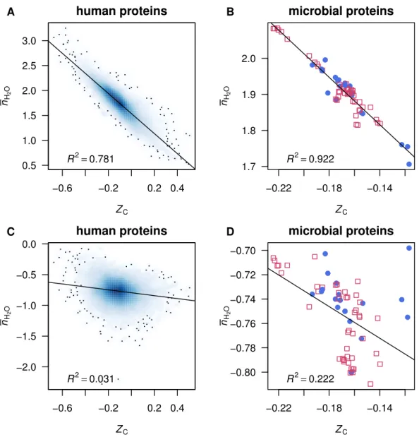
as seen inFigs. 1Aand1B, there is a high correlation betweenZCof protein molecules and
¯nH2Oin the reactions to form the proteins from Basis I (note that the choice of basis species
affects only ¯nH2Oand notZC). Because of this stoichiometric interdependence, changes in
either redox or hydration potential, while holding the chemical potentials of the remaining basis species constant, have correlated effects on the energetics of chemical transformations (see ‘Comparison with inorganic basis species’ below). A different set of basis species can be chosen that reduces this correlation and affords a more informative description of the compositional changes in proteomic transformations.
Basis II
In this exploratory study, we restrict attention to at most two variables, with the implication that the others are held constant. In a subcellular setting, assuming that the chemical
potentials of CO2, NH3 and H2S do not change during a proteomic transformation,
as implied by varying the chemical potentials of O2 and H2O in Basis I, may be less
appropriate than assuming constant chemical potentials of more complex metabolites. In thermodynamic models for systems of proteins, constant chemical activities of chemical components having the compositions of amino acids might be a reasonable provision.
Although 1140 3-way combinations can be made of the 20 common proteinogenic amino acids, only 324 of the combinations contain cysteine and/or methionine (one of these is
required to provide sulfur), and of these only 300, when combined with O2and H2O, are
compositionally nondegenerate. The slope, intercept andR2of the linear least-squares fits
betweenZCandnH2Ousing each possible basis containing O2, H2O and three amino acids
are listed in fileAAbasis.csvinDataset S1. Many of these combinations have lowerR2and
lower slopes than found for Basis I (Figs. 1Aand1B), indicating a decreased correlation.
From those with a lower correlation, but not the lowest, the basis including cysteine (Cys),
glutamic acid (Glu), glutamine (Gln), O2and H2O (Basis II) has been selected for use
in this study. The scatterplots and fits between ZCandnH2O using Basis II are shown in
Figs. 1Cand1D.
A secondary consideration in choosing this basis instead of others with even lowerR2
is the centrality of glutamine and glutamic acid in many metabolic pathways (e.g.,
−0.6 −0.2 0.2 0.4 0.5
1.0 1.5 2.0 2.5 3.0
ZC
nH
2
O
human proteins
R2=0.781
A
●● ●
● ●
●
● ●
● ● ●
● ● ●
● ● ●
● ●
●
−0.22 −0.18 −0.14 1.7
1.8 1.9 2.0
ZC
nH
2
O
microbial proteins
R2=0.922
B
−0.6 −0.2 0.2 0.4
−2.0 −1.5 −1.0 −0.5 0.0
ZC
nH
2
O
human proteins
R2=0.031
C
●● ●
● ● ●
● ●
● ● ●
●
● ●
●
● ●
● ● ●
−0.22 −0.18 −0.14 −0.80
−0.78 −0.76 −0.74 −0.72 −0.70
ZC
nH
2
O
microbial proteins
R2=0.222
D
Figure 1 Scatterplots of average oxidation state of carbon (ZC) and water demand per residue (nH2O). Data are plotted for (A, C) individual human proteins and (B,D) mean composition of proteins from mi-crobial genomes, withnH2Ocomputed using (A, B) Basis I (Reaction (R1)) or (C, D) Basis II (Reaction (R2)). Linear least-squares fits andR2values are shown. In (A) and (C), the intensity of shading corre-sponds to density of points, produced using thesmoothScatter()function of R graphics (R Core Team,
2016). The label in plot (A) identifies a particular protein, MUC1, which is used for the example calcula-tions (see Reaccalcula-tions (R3) and (R4)).
basis species is neither uniquely determined nor necessarily optimal for a thermodynamic description of any particular system. More experience with thermodynamic modeling and better biochemical intuition will likely provide reasons to refine these calculations using a different basis, perhaps including metabolites other than amino acids.
A general formation reaction using Basis II is
nCysC3H7NO2S+nGluC5H9NO4+nGlnC5H10N2O3
where the reaction coefficients (nCys,nGlu,nGln,nH2OandnO2) can be obtained by solving
3 5 5 0 0
7 9 10 2 0
1 1 2 0 0
2 4 3 1 2
1 0 0 0 0
×
nCys nGlu nGln nH2O nO2
=
c h n o s
. (2)
Although the definition of basis species requires that they are themselves compositionally nondegenerate, the matrix equation emphasizes the interdependence of the stoichiometric reaction coefficients. A consequence of this multiple dependence is that single variables
such asnO2 andnH2O are not simple variables, but are influenced by both the chemical
composition of the protein and the choice of basis species used to describe the system.
The combination of molecules shown in Reaction (R2) does not represent the actual
mechanism of synthesis of the proteins. Instead, reactions such as this account for mass-conservation requirements and permit the subsequent generation of thermodynamic models for the potential for formation of different proteins as a function of system
parameters (i.e., chemical potentials of O2and H2O).
As an example of a specific calculation, consider the following reaction for MUC1, a
chromatin-binding protein that is highly up-expressed in CRC cells (Knol et al.,2014).
7C3H7NO2S+535.6C5H9NO4+515.2C5H10N2O3
→C5275H8231N1573O1762S7+895.2H2O+522.4O2. (R3)
As with the other reactions shown above, this reaction is not a mechanism, but represents the stoichiometric requirements for the formation from the basis species of one mole of the
protein. Water is released in Reaction (R3), so the water demand (nH2O) is negative. The
length of this protein is 1,255 amino acid residues, giving the water demand per residue,
nH2O= −895.2/1,255= −0.71. The average oxidation state of carbon (ZC) in MUC1,
which does not depend on the choice of basis species, is 0.005 (Eq. 1). The value ofZC
indicates that MUC1 is a relatively highly oxidized protein, while itsnH2Oplaces it near the
median water demand for up-expressed proteins in cancer in this dataset (seeFig. 2Abelow).
Thermodynamic calculations
Standard molal thermodynamic properties of the amino acids and unfolded proteins
estimated using amino acid group additivity were calculated as described byDick, LaRowe
& Helgeson (2006), taking account of updated values for the methionine sidechain
group (LaRowe & Dick,2012). In this study, the Gibbs energies of hypothetically
non-ionized proteins were used, and calculations were carried out at 37 ◦C and 1 bar. The
temperature dependence of standard Gibbs energies was calculated using the revised
Helgeson–Kirkham–Flowers (HKF) equations of state (Helgeson, Kirkham & Flowers,1981;
Tanger IV & Helgeson,1988). Thermodynamic properties for O2(gas) were calculated using
data fromWagman et al.(1982) and the Maier–Kelley heat capacity function (Kelley,1960).
● ● ● ● ● ● ● ● ● ● ● ● ● ● ● ● ● ● ● ● ● ● ● ● ● ● ● ● ● ● ● ● ● ● ● ● ● ● ● ● ● ● ● ● ● ● ● ● ● ● ●
−0.25 −0.15 −0.05 −0.9 −0.8 −0.7 −0.6 −0.5 −0.4 ZC nH 2 O
chromatin−binding C / A
KW A+14 MUC1 A ● ● ● ● ● ● ● ● ● ● ● ● ● ● ● ● ● ● ● ● ● ●● ● ● ● ● ● ● ● ● ● ● ● ● ● ● ● ● ● ● ● ● ●
−0.2 −0.1 0.0 0.1 0.2 −1.0 −0.9 −0.8 −0.7 −0.6 −0.5 −0.4 ZC nH 2 O
tissue secretome T / N
WKP+14 B ● ● ● ● ● ● ● ● ● ● ● ● ● ● ● ● ● ●● ● ● ● ● ● ● ● ● ● ● ● ● ● ● ● ● ● ● ● ● ● ● ● ● ● ● ● ● ● ● ●● ● ● ● ● ● ● ● ● ● ● ● ● ● ● ● ● ● ● ● ● ● ● ● ● ● ● ●● ● ● ● ● ● ● ● ● ● ● ● ● ● ● ● ● ● ● ● ● ● ● ●● ● ● ● ● ● ● ● ● ● ● ● ● ● ● ● ● ● ● ● ● ● ● ● ● ● ● ● ● ● ● ● ● ● ● ● ● ● ● ● ● ● ● ● ● ● ● ● ● ● ● ● ● ● ● ● ● ●● ● ● ● ● ● ● ● ● ● ● ● ● ● ● ● ●● ● ● ● ● ● ● ● ● ● ● ● ● ● ● ● ● ● ● ● ● ● ● ● ● ● ● ● ● ● ● ● ● ● ● ● ● ● ● ● ● ● ● ● ● ● ● ● ● ● ● ● ● ● ● ● ● ● ● ● ● ● ● ● ● ● ● ● ● ● ● ● ● ● ● ● ● ● ● ● ● ● ● ● ● ● ● ● ● ● ● ● ● ● ● ● ● ● ● ● ● ● ● ● ● ● ● ● ● ● ● ● ● ● ● ● ● ● ● ● ● ● ● ●● ● ● ● ● ● ● ● ● ● ● ● ● ● ● ● ● ● ● ● ● ● ● ● ● ● ● ● ● ● ● ● ● ● ● ● ● ● ● ● ● ● ● ● ● ● ●● ● ● ● ● ● ● ● ● ● ● ● ● ● ● ● ● ● ● ● ● ● ● ● ● ● ● ● ● ●● ● ● ● ● ● ● ● ●●● ● ● ● ● ● ● ● ● ● ● ● ● ● ● ● ● ● ● ● ● ● ● ● ● ● ●● ● ● ● ● ● ● ● ● ● ● ● ● ● ● ● ● ● ● ● ● ● ● ● ● ● ● ● ● ● ● ● ● ● ● ● ● ● ● ● ● ● ●● ● ● ● ● ● ● ● ● ● ● ● ● ● ● ● ● ● ● ● ● ● ● ● ● ● ● ● ● ● ● ● ●● ● ● ● ● ● ● ● ● ● ● ● ● ● ● ● ● ● ● ● ● ● ● ● ● ● ● ● ● ● ● ● ● ● ● ● ● ● ● ● ● ● ● ● ● ● ●● ● ● ● ● ● ● ● ● ● ● ● ●● ● ● ● ● ● ● ● ● ● ●● ● ● ● ● ● ● ● ● ● ● ● ● ● ● ● ● ● ● ● ● ● ● ● ● ● ● ● ● ● ● ● ● ● ● ● ● ● ● ● ●● ● ●●●● ● ● ● ● ● ● ● ● ●● ● ● ● ● ● ● ● ● ● ● ● ● ● ● ● ● ● ● ● ● ● ● ● ● ● ● ● ● ● ● ● ● ● ● ● ● ● ● ● ● ● ● ● ● ● ● ● ● ● ● ● ● ● ● ● ● ● ● ● ● ● ● ● ● ● ● ● ● ● ● ● ● ● ● ● ● ● ● ● ● ● ● ● ● ● ●●● ● ● ● ● ● ● ● ● ● ● ● ● ● ● ● ● ● ● ● ● ● ● ● ● ● ● ● ● ● ● ● ● ● ● ● ● ● ● ● ● ● ● ● ● ● ● ● ● ● ● ● ● ● ● ● ● ● ● ● ● ● ● ● ● ● ● ● ● ● ● ● ● ● ● ● ● ● ● ● ● ● ● ● ● ●● ● ● ● ● ● ● ● ● ● ● ● ● ● ● ● ● ● ● ● ● ●● ● ● ● ● ● ● ● ● ● ● ● ● ● ● ● ● ● ● ●●● ● ● ● ●● ● ● ● ● ● ● ● ●● ● ●● ●● ● ● ● ● ● ● ● ● ● ● ● ● ● ● ● ● ● ● ● ● ● ● ● ● ● ● ● ● ● ● ● ● ● ● ● ● ● ● ● ● ● ● ● ● ● ● ● ● ● ● ● ● ● ● ● ● ● ● ● ● ● ● ● ● ● ● ● ● ● ● ● ● ● ● ● ● ● ● ● ● ● ● ● ● ● ● ● ●● ● ● ● ● ● ● ● ● ● ● ● ● ● ● ● ● ● ● ● ● ● ● ● ● ● ● ● ● ● ● ● ● ● ● ● ● ● ● ● ● ● ● ● ● ● ● ● ● ● ● ● ● ● ● ● ● ● ● ● ● ● ● ● ● ● ● ● ● ● ● ● ● ● ● ● ● ● ● ● ● ● ● ● ● ● ● ● ● ● ● ● ● ● ● ● ● ● ● ● ● ● ● ● ● ● ● ● ● ● ●● ● ●●● ● ●
−0.4 −0.2 0.0 0.2 0.4 −1.2 −1.0 −0.8 −0.6 −0.4 ZC nH 2 O
adenoma / normal
WDO+15_A.N
C
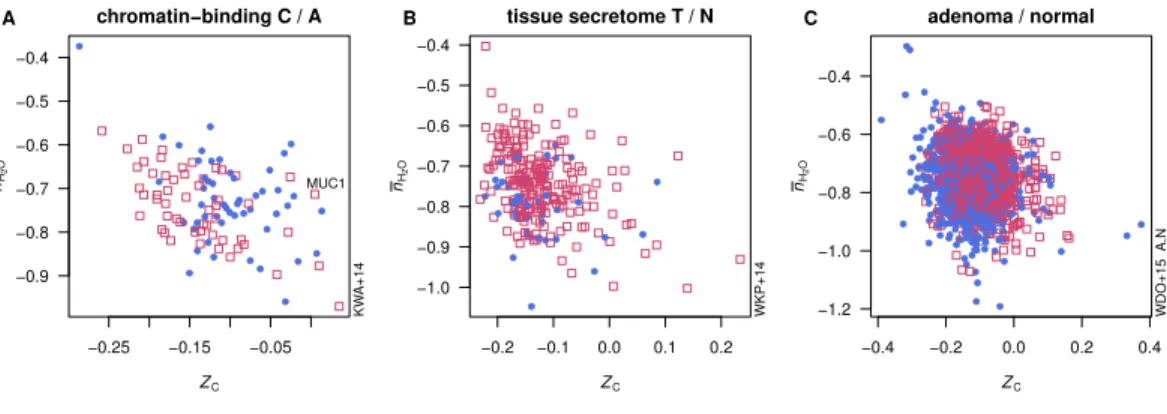
Figure 2 Average oxidation state of carbon (ZC) and water demand per residue (nH2O) for proteins
in selected datasets. Open red squares represent proteins enriched in tumors or more advanced cancer stages, and filled blue circles represent proteins enriched in normal tissue or less advanced cancer stages.
subroutines from the SUPCRT92 package (Johnson, Oelkers & Helgeson,1992), as provided
in the CHNOSZ package (Dick,2008).
Chemical affinities of reactions were calculated using activities of amino acids in the
basis equal to 10−4, and activities of proteins equal to 1/(protein length) (i.e., unit activity
of amino acid residues). Continuing with the example of Reaction (R3), an estimate of the
standard Gibbs energy (1Gof) of the aqueous protein molecule (Dick, LaRowe & Helgeson,
2006;LaRowe & Dick,2012) at 37 ◦C is−40,974 kcal/mol; combined with the standard
Gibbs energies of the basis species, this give a standard Gibbs energy of reaction (1Gor)
equal to 66,889 kcal/mol. At logaH2O=0 and logfO2= −65, with activities of the amino
acid basis species equal to 10−4, the overall Gibbs energy (1Gr) is 24,701 kcal/mol. The
negative of this value is the chemical affinity (A) of the reaction. The per-residue chemical
affinity for formation of protein MUC1 in the stated conditions is−19.7 kcal/mol. (This
calculation can be reproduced using the functionreaction()in fileplot.RinDataset S1.)
In a given system, proteins with higher (more positive) chemical affinity are relatively energetically stabilized, and theoretically have a higher propensity to be formed. Therefore, the differences in affinities reflect not only the amino acid compositions of the protein molecules but also the potential for local environmental conditions to influence the relative abundances of proteins.
Weighted rank difference
The contours on relative stability diagrams for the groups of differentially expressed
proteins (see Fig. 6below) depict the weighted rank differences of chemical affinities
of formation of proteins. To illustrate this calculation, consider a hypothetical system composed of 3 proteins with higher expression in cancer (C) and 4 with higher expression in normal samples (down-expressed in cancer, i.e., having higher expression in a healthy
state) (H). Suppose that under one set of conditions (i.e., specified logaH2O and logfO2),
the per-residue affinities of the proteins give the following ranking in ascending order (I):
C C C H H H H
This gives as the sum of ranks for up-expressed (C) proteinsP
rC=6, and for
down-expressed (H) proteinsP
rH=22. The difference in sum of ranks is1rC−H= −16; the
negative value is associated with a higher rank sum for the down-expressed proteins, indicating that these as a group are more stable than the down-expressed proteins. In a second set of conditions, we might have (II):
H H H H C C C
1 2 3 4 5 6 7
Here, the difference of rank sums is1rC−H=18−10=8.
For systems where the numbers of proteins in the two groups are equal, the maximum possible differences in rank sums would have equal absolute values, but that is not the case in this and other systems having unequal numbers of up- and down-expressed proteins. To characterize these datasets, the weighted rank-sum difference can be calculated using
1r=2nH n
X
rC− nC
n
X
rH
(3)
wherenH,nCandnare the numbers of down-expressed, up-expressed, and total proteins
in the comparison. In the example here, we havenH/n=4/7 andnC/n=3/7.Equation (3)
then gives1r= −12 and1r=12, respectively, for conditions (I) and (II) above, showing
equal weighted rank-sum differences for the two extreme rankings.
We can also consider a situation where the ranks of the proteins are evenly distributed:
H C H C H C H
1 2 3 4 5 6 7
Here the absolute difference of rank sums is1rC−H=12−16= −4, but the weighted
rank-sum difference is1r=0. The zero value for an even distribution and the opposite
values for the two extremes demonstrate the applicability of this weighting scheme.
Software and data availability
All statistical and thermodynamic calculations were performed using R (R Core Team,
2016). Thermodynamic calculations were carried out using R package CHNOSZ (Dick,
2008). Effect sizes (see below) were calculated using R package orddom (Rogmann,2013).
Figures were generated using CHNOSZ and graphical functions available in R together
with the R package colorspace (Ihaka et al.,2015) for constructing an HCL-based color
palette (Zeileis, Hornik & Murrell,2009). With the mentioned packages installed,Table 1
and the figures in this paper can be reproduced using the code (plot.R) and data files
(*.csv) inDataset S1.
RESULTS
Compositional comparisons of human proteins
Comparisons of proteome composition in terms of average oxidation state of carbon
(ZC) and water demand per residue (¯nH2O) are presented inFig. 2andTable 1.Figure 2
studies. Each of these exhibits a strongly differential trend inZCor¯nH2Othat can be visually
identified. InFig. 2A, chromatin-binding proteins highly expressed in carcinoma (Knol et
al.,2014) as a group exhibit a lowerZCthan those found to be more abundant in adenoma.
InFig. 2B, proteins relatively highly expressed in epithelial cells in adenoma (Uzozie et al.,
2014) tend to have higher¯nH2Othan the proteins more highly expressed in paired normal
tissues. Differentially expressed proteins between adenoma and normal tissue identified in
a recent deep-proteome analysis (Wiśniewski et al.,2015) are compared inFig. 2C, showing
that proteins up-expressed in adenoma are relatively oxidized (i.e., have higherZC).
In order to quantify these differences,Table 1shows the numbers of proteins in each
comparison (n1for normal or less advanced cancer stage;n2for tumor or more advanced
cancer stage), differences of means (MD), common language effect size as percentages
(ES), andp-values calculated using the Wilcoxon rank sum test. This non-parametric test
is suitable for data which may not be normally distributed. For a given experiment, the common language effect size, or probability of superiority, describes the probability that
ZCornH2Oof a protein is higher in the cancer group than in the normal group. That is,
percent values of the ES greater than (or less than) 50 indicate a greater proportion of
pairwise higher (or lower)ZCornH2Oof proteins in then2compared ton1groups. The
ES and p-value are used here to allow for a subjective assessment of the compositional
differences. ES values≥60 or≤40 andp-values < 0.05 are highlighted in the table. The
corresponding mean differences are underlined forp< 0.05, or bolded if ES is also≥60 or
≤40. These cutoffs highlight datasets with the largest and most significant differences in
ZCand¯nH2O. Mean and median values ofZC and¯nH2O are given in filesummary.csvin
Dataset S1.
Counting the underlined and bolded MD values inTable 1, the number of datasets with
a significant difference inZC(18) is greater than those with a significant difference in¯nH2O
(10). Of the 10 unique studies yielding at least one dataset with a significant difference
inZCin a comparison with normal tissue, 8 exhibit a higher mean value in adenoma or
carcinoma compared to normal tissue. One of the other studies (Besson et al.,2011) has
datasets with higher meanZCin proteins up-expressed in adenoma, but lower meanZCin
proteins up-expressed in stage II and III carcinoma, compared to normal tissue. A second
study, which analyzed proteins in stromal cells (Li et al.,2016), shows a significantly lower
ZCin adenoma compared to normal tissue.
Most of the studies analyzed proteins in whole or microdissected tissue, but two datasets in studies from the same laboratory represent the nuclear matrix or chromatin-binding
fraction (Albrethsen et al.,2010;Knol et al.,2014). These two datasets give lower meanZC
of proteins more highly expressed in carcinoma than adenoma. One other dataset has a
lower meanZCof proteins up-expressed in carcinoma compared to adenoma (Wiśniewski
et al.,2015), and one has a higher mean value (Mikula et al.,2011).
The datasets with a significant difference in ¯nH2O all show higher mean values for
proteins in adenoma (5 datasets) or carcinoma (3 datasets) compared to normal tissue,
up- expressed compared to down-expressed serum biomarker candidates (Jimenez et al.,
2014). Interestingly, none of the datasets with a significant difference in¯nH2Ocorresponds
to a carcinoma/adenoma comparison.
Natural variability inherent in the heterogeneity of tumors, as well as differences in
experimental design and technical analysis, may underlie the opposite trends inZCbetween
some datasets that compare the same stages of cancer. However, there is a preponderance
of datasets with higher values ofZCand¯nH2Ofor the proteins up-expressed in adenoma or
carcinoma compared to normal tissue.
Compositional comparisons of microbial proteins
Summary data on microbial populations from four studies were selected for comparison
here. First, in a study of 16S RNA of fecal microbiota,Wang et al.(2012) reported genera
that are significantly increased or decreased in CRC compared to healthy patients. In order to compare the chemical compositions of the microbial populations, single species
with sequenced genomes were chosen to represent each of these genera (see Table 2).
Where possible, the species selected are those mentioned byWang et al.(2012) as being
significantly altered, or are species reported in other studies to be present in healthy or
cancer states (seeTable 2).
In the second study considered (Zeller et al.,2014), changes in the metagenomic
abundance of fecal microbiota associated with CRC were analyzed for their potential
as a biosignature for cancer detection. The species shown in Fig. 1A ofZeller et al.(2014)
with a log odds ratio greater than 0.15 were selected for comparison, and are listed in Table 3.Zeller et al.(2014) found a strong enrichment of Fusobacteriumin cancer,
consistent with previous reports (Kostic et al.,2012;Castellarin et al.,2012). In a third
study,Candela et al. (2014) reported the findings of a network analysis that identified
5 microbial ‘‘co-abundance groups’’ at the genus level. As before, single representative
species were selected in this study, and are listed in Table 2. Except for the presence of
Fusobacterium, the co-abundance groups show little genus-level overlap with community profiles derived from the previous two studies.
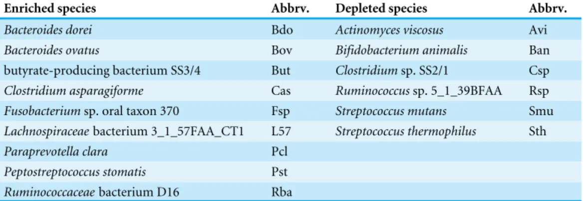
Finally,Table 4lists the ‘‘best aligned strain’’ from Supplementary Dataset 5 ofFeng et
al.(2015) for all species shown there with negative enrichment in cancer, and for selected
species with positive enrichment in cancer. Although every uniquely named strain given byFeng et al.(2015) was used in the comparisons below (n=44; seeFig. 3Dbelow), for clarity only the up-enriched species that appear in the calculated stability diagram (see
Fig. 4Dbelow) are listed inTable 4and labeled inFig. 3D. Filemicrobes.csvinDataset
S1contains the complete list of Bioproject IDs and calculated ZC and ¯nH2O for all the
microbial species considered here.
For each of the microbial species listed inTables 2–4, a mean protein composition
was calculated by combining amino acid sequences of all proteins downloaded from the NCBI genome page associated with the Bioproject IDs shown in the Tables (see file
Table 2 Microbial species selected as models for genera and co-abundance groups that differ between CRC and healthy patients.
Phylum Species Abbrv. Bioproject Refs.
Model species for genera significantly higher in healthy patientsa
Bacteroidetes Bacteroides vulgatusATCC 8482 Bvu PRJNA13378 c
Bacteroidetes Bacteroides uniformisATCC 8492 Bun PRJNA18195 c
Firmicutes Roseburia intestinalisL1-82 (DSM 14610) Rin PRJNA30005 d
Bacteroidetes Alistipes indistinctusYIT 12060 Ain PRJNA46373 c
Firmicutes Eubacterium rectaleATCC 33656 Ere PRJNA29071 e
Proteobacteria Parasutterella excrementihominisYIT 11859 Pex PRJNA48497 f
Model species for genera significantly higher in CRC patientsa
Bacteroidetes Porphyromonas gingivalisW83 Pgi PRJNA48 g
Proteobacteria Escherichia coliNC101 Eco PRJNA47121 c,h
Firmicutes Enterococcus faecalisV583 Efa PRJNA57669 c
Firmicutes Streptococcus infantariusATCC BAA-102 Sin PRJNA20527 i
Firmicutes Peptostreptococcus stomatisDSM 17678 Pst PRJNA34073 j
Bacteroidetes Bacteroides fragilisYCH46 Bfr PRJNA58195 g
Model species for protective co-abundance groupsb
Actinobacteria Bifidobacterium longumNCC2705 Blo PRJNA57939 g,k
Firmicutes Faecalibacterium prausnitziiSL3/3 Fpr PRJNA39151 e,l
Model species for pro-carcinogenic co-abundance groupsb
Fusobacteria Fusobacterium nucleatumATCC 23726 Fnu PRJNA49043 m,n
Bacteroidetes Prevotella copriDSM 18205 Pco PRJNA30025 k,o
Firmicutes Coprobacillussp. D7 Csp PRJNA32495 h
Notes.
aGenus identification from Table 2 ofWang et al.(2012). Based on comments inWang et al.(2012),Bacteroidesis represented
here by two species (B. vulgatusandB. uniformis) in healthy patients, and one species (B. fragilis) in CRC patients.
bGenus-level definition of co-abundance groups fromCandela et al.(2014).
cWang et al.(2012); species closely related to 16S rRNA-derived operational taxonomic units (OTUs; Fig. 2 ofWang et al.,
2012) or otherwise mentioned by those authors (E. faecalis).
dDuncan et al.(2002). eLouis & Flint(2007). fNagai et al.(2009). gChen et al.(2012). hCandela et al.(2014).
iBiarc et al.(2004). jZeller et al.(2014). kWeir et al.(2013).
lSokol et al.(2008). mCastellarin et al.(2012).
nKostic et al.(2012).
ocf.Chen et al.(2012) andCandela et al.(2014) (more abundant in CRC patients);Weir et al.(2013) (more abundant in healthy
subjects).
signals in protein composition. Mean amino acid compositions or amino acid frequencies deduced from microbial genomes, calculated without weighting for actual protein abundance, have been used in many studies making evolutionary and/or environmental
comparisons (e.g.,Tekaia & Yeramian,2006;Zeldovich, Berezovsky & Shakhnovich,2007;
Brbić et al., 2015). In the future, more refined calculations may be possible by using genome-wide estimates of protein expression levels based on codon usage patterns (e.g.,
Table 3 Species from a consensus microbial signature for CRC classification of fecal metagenomes
(Zeller et al.,2014).Only species reported as having a log odds ratio larger than±0.15 are listed here,
to-gether with strains and Bioproject IDs used as models in the present study.
Species Strain Abbrv. Bioproject
Higher in CRC patients
Fusobacterium nucleatumsubsp. vincentii ATCC 49256 Fnv PRJNA1419
Fusobacterium nucleatumsubsp. animalis D11 Fna PRJNA32501
Peptostreptococcus stomatis DSM 17678 Pst PRJNA34073
Porphyromonas asaccharolytica DSM 20707 Pas PRJNA51745
Clostridium symbiosum ATCC 14940 Csy PRJNA18183
Clostridium hylemonae DSM 15053 Chy PRJNA30369
Lactobacillus salivarius ATCC 11741 Lsa PRJNA31503
Higher in healthy patients
Clostridium scindens ATCC 35704 Csc PRJNA18175
Eubacterium eligens ATCC 27750 Eel PRJNA29073
Methanosphaera stadtmanae DSM 3091 Mst PRJNA15579
Phascolarctobacterium succinatutens YIT 12067 Psu PRJNA48505
unclassifiedRuminococcussp. ATCC 29149(a) Rsp PRJNA18179
Streptococcus salivarius SK126 Ssa PRJNA34091
Notes.
aR. gnavus.
Table 4 Selected microbial species enriched or depleted in stool samples from cancer patients com-pared to healthy controls (Feng et al.,2015).
Enriched species Abbrv. Depleted species Abbrv.
Bacteroides dorei Bdo Actinomyces viscosus Avi
Bacteroides ovatus Bov Bifidobacterium animalis Ban
butyrate-producing bacterium SS3/4 But Clostridiumsp. SS2/1 Csp
Clostridium asparagiforme Cas Ruminococcussp. 5_1_39BFAA Rsp
Fusobacteriumsp. oral taxon 370 Fsp Streptococcus mutans Smu
Lachnospiraceaebacterium 3_1_57FAA_CT1 L57 Streptococcus thermophilus Sth
Paraprevotella clara Pcl
Peptostreptococcus stomatis Pst
Ruminococcaceaebacterium D16 Rba
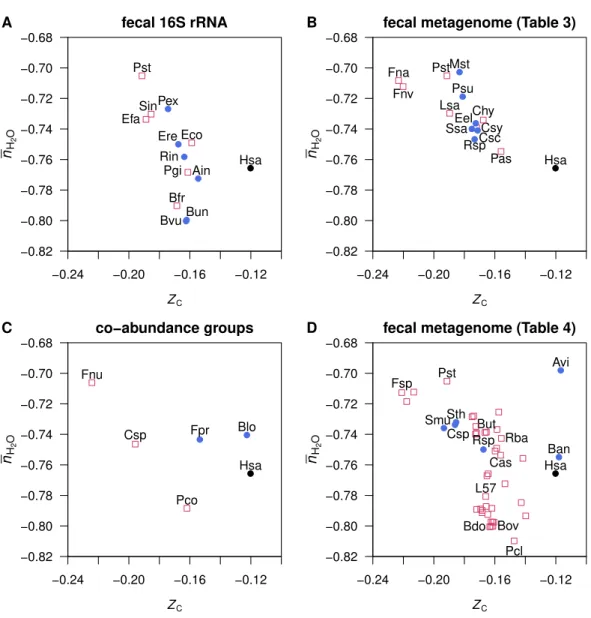
The water demand per residue (nH2O) vs. oxidation state of carbon (ZC) in the mean
amino acid compositions of proteins from all of the microbial species considered here are
plotted inFigs. 1Band1D, and for individual datasets inFig. 3. The groups of proteins
in the microbes enriched in cancer patients have somewhat lowerZCthan those enriched
in healthy donors in the same study. The dataset fromFeng et al.(2015) (Fig. 3D) shows
a more complex distribution, where the microbes with a relative enrichment in healthy
individuals form two clusters at high and lowZC. TheFusobacteriumspecies identified in
the studies ofZeller et al.(2014),Candela et al.(2014) andFeng et al.(2015) have the lowest
−0.24 −0.20 −0.16 −0.12 −0.82 −0.80 −0.78 −0.76 −0.74 −0.72 −0.70 −0.68 ZC nH 2 O ● Hsa ●
Bvu●Bun ● Rin ● Ain ● Ere ● Pex Pgi Eco Efa Sin Pst Bfr
fecal 16S rRNA A
−0.24 −0.20 −0.16 −0.12 −0.82 −0.80 −0.78 −0.76 −0.74 −0.72 −0.70 −0.68 ZC nH 2 O ● Hsa Fnv Fna Pst Pas Csy Chy Lsa ● Csc ● Eel ● Mst ● Psu ● Rsp ● Ssa
fecal metagenome (Table 3) B
−0.24 −0.20 −0.16 −0.12 −0.82 −0.80 −0.78 −0.76 −0.74 −0.72 −0.70 −0.68 ZC nH 2 O ● Hsa ● Blo ● Fpr Fnu Pco Csp co−abundance groups C
−0.24 −0.20 −0.16 −0.12 −0.82 −0.80 −0.78 −0.76 −0.74 −0.72 −0.70 −0.68 ZC nH 2 O ● Hsa Bdo Bov But Cas Fsp L57 Pcl Pst Rba ● Avi ● Ban ● Csp ● Rsp ●
SmuSth●
fecal metagenome (Table 4) D
Figure 3 Average oxidation state of carbon (ZC) and water demand per residue (nH2O) for mean amino
acid compositions of proteins in genomes of normal- and cancer-enriched microbes.Data are shown for representative species for (A) microbial genera identified in fecal 16s RNA (Wang et al.,2012; Ta-ble 2top), (B) microbial signatures in fecal metagenomes (Zeller et al.,2014;Table 3), (C) microbial co-abundance groups (Candela et al.,2014;Table 2bottom), and (D) best aligned strains to metagenomic linkage groups in fecal samples (Feng et al.,2015;Table 4). The mean amino acid composition of proteins in theHomo sapiensgenome (Hsa) is also shown.
plotted inFig. 3, revealing a higherZC than any of the mean microbial proteins except
forActinomyces viscosusandBifidobacterium animalis, identified in the study ofFeng et al.
(2015) (Fig. 3D). The tendency for microbial organisms to be composed of more reduced biomolecules than the host may reflect the relatively reducing conditions in the gut.
Thermodynamic descriptions: background
−75 −70 −65 −60 −55 −10 −5 0 5 10
logfO2(g)
lo g aH 2 O ( liq ) Bvu Bun Rin Ain Pex Eco Efa Pst
fecal 16S rRNA A
−75 −70 −65 −60 −55
−10 −5 0 5 10
logfO2(g)
lo g aH 2 O ( liq ) Fnv Fna Pas Chy Eel Psu Rsp
fecal metagenome (Table 3) B
−75 −70 −65 −60 −55
−10 −5 0 5 10
logfO2(g)
lo g aH 2 O ( liq ) Blo Fpr Fnu Pco Csp co−abundance groups C
−75 −70 −65 −60 −55
−10 −5 0 5 10
logfO2(g)
lo g aH 2 O ( liq ) BdoBov But Cas Fsp L57 Pcl Pst Rba Avi Ban
fecal metagenome (Table 4) D
−75 −70 −65 −60 −55
−10 −5 0 5 10
logfO2(g)
lo g aH 2 O ( liq )
cumulative stability count E
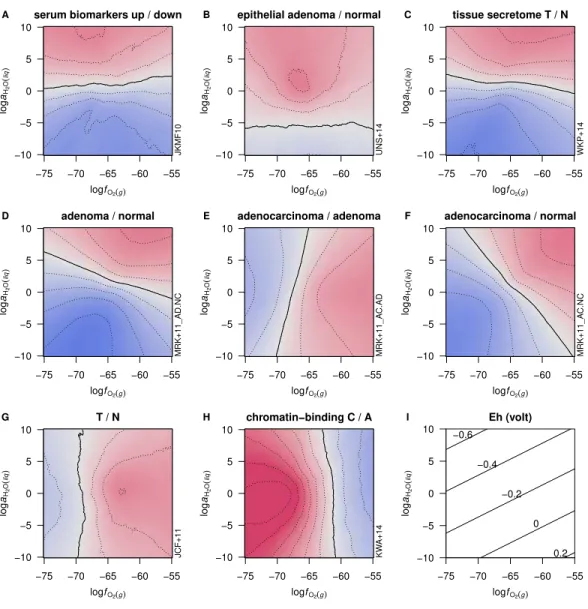
Figure 4 Maximal relative stability diagrams for mean microbial protein compositions.Each stabil-ity field in these diagrams shows the ranges of oxygen fugacstabil-ity and water activstabil-ity (in log units: logfO2and
logaH2O) where the mean protein composition from the labeled microbial species has a higher per-residue
affinity (lower Gibbs energy) of formation than the others. Blue and red shading designate microbes rel-atively enriched in samples from healthy donors and cancer patients, respectively. Plot (E) is a compos-ite figure in which the intensity of shading corresponds to the number of overlapping healthy- or cancer-enriched microbes in the preceding diagrams.
By combining both stoichiometric and energetic variables, a thermodynamic description of proteomic data reveals possible biochemical constraints that may arise within cells and in tumor microenvironments. To give an example of how relative stabilities of up- and down-expressed proteins in a proteomic dataset can be calculated as a function of chemical
potentials, consider Reaction (R3) above written for the formation of one mole of MUC1.
In order to compare proteins of different lengths, the formula of the protein is written per residue. The corresponding reaction is then
0.006C3H7NO2S+0.427C5H9NO4+0.411C5H10N2O3
→C4.203H8.557N1.253O2.403S0.006+0.714H2O+0.416O2. (R4)
An expression for the chemical affinity (Kondepudi & Prigogine,1998;Helgeson et al.,2009)
of Reaction (R4) is
A=2.303RTlog(K/Q) (4)
where 2.303 is shorthand for the natural logarithm of 10,Ris the gas constant,Tis
tempera-ture, log represents the common (decimal) logarithm, and the activity quotientQis given by
logQ=logaC4.203H8.557N1.253O2.403S0.006+0.714logaH2O+0.416logfO2