www.nonlin-processes-geophys.net/21/1075/2014/ doi:10.5194/npg-21-1075-2014
© Author(s) 2014. CC Attribution 3.0 License.
Wavevector anisotropy of plasma turbulence at ion kinetic scales:
solar wind observations and hybrid simulations
H. Comi¸sel1,2, Y. Narita3,4, and U. Motschmann1,5
1Institut für Theoretische Physik, Technische Universität Braunschweig, Mendelssohnstr. 3, 38106 Braunschweig, Germany 2Institute for Space Sciences, Atomi¸stilor 409, P.O. Box MG-23, Bucharest-M˘agurele 77125, Romania
3Space Research Institute, Austrian Academy of Sciences, Schmiedlstr. 6, 8042 Graz, Austria
4Institut für Geophysik und extraterrestrische Physik, Technische Universität Braunschweig, Mendelssohnstr. 3, 38106 Braunschweig, Germany
5Deutsches Zentrum für Luft- und Raumfahrt, Institut für Planetenforschung, Rutherfordstr. 2, 12489 Berlin, Germany
Correspondence to:H. Comi¸sel ([email protected])
Received: 10 July 2014 – Published in Nonlin. Processes Geophys. Discuss.: 12 August 2014 Revised: 8 October 2014 – Accepted: 15 October 2014 – Published: 11 November 2014
Abstract.Wavevector anisotropy of ion-scale plasma turbu-lence is studied at various values of ion beta. Two comple-mentary methods are used. One is multi-point measurements of magnetic field in the near-Earth solar wind as provided by the Cluster spacecraft mission, and the other is hybrid numer-ical simulation of two-dimensional plasma turbulence. Both methods demonstrate that the wavevector anisotropy is re-duced with increasing values of ion beta. Furthermore, the numerical simulation study shows the existence of a scaling law between ion beta and the wavevector anisotropy of the fluctuating magnetic field that is controlled by the thermal or hybrid particle-in-cell simulation noise. Likewise, there is weak evidence that the power-law scaling can be extended to the turbulent fluctuating cascade. This fact can be used to construct a diagnostic tool to determine or to constrain ion beta using multi-point magnetic field measurements in space.
1 Introduction
Wavevector anisotropy appears in collisionless plasma turbu-lence whenever a large-scale magnetic field is present.
Anisotropy is characterized by extension or elongation of the energy spectrum in the direction parallel or perpendicular to the large-scale field. Examples of wavevector anisotropy can be found in near-Earth solar wind (e.g., Matthaeus et al., 1990; Chen et al., 2012), astrophysical systems such as
(Valentini et al., 2010; Verscharen et al., 2012; Comi¸sel et al., 2013), gyrokinetic treatment (Howes et al., 2011), and whistler turbulence on electron scales (Saito et al., 2008). Furthermore, particle-in-cell simulations show the wavevec-tor anisotropy of whistler turbulence at electron-scale wave-lengths decreases with increasing electron beta (Gary et al., 2010; Saito et al., 2010; Saito and Gary, 2012; Chang et al., 2013), which motivates our study here.
Here we propose a scenario that ion beta is one of the con-trol parameters such that wavevector anisotropy in the ion kinetic regime is reduced with increasing values of ion beta.
Ion betaβiis defined here as
βi=
2µ0nikBTi
B02 , (1)
where the symbols denoteµ0the permeability of free space,
nithe ion number density,kBthe Boltzmann constant,Tithe ion temperature, andB0the mean magnetic field magnitude. By extending the method and the result obtained in Narita et al. (2014) (hereafter NCM14), we find a transition in the wavevector anisotropy as a function of ion beta. While the qualitative picture of ion beta dependence is demonstrated in NCM14, this article presents a more systematic survey of ion beta dependence both in spacecraft measurements and direct numerical simulations. Our goal is to search for a scaling law of the wavevector anisotropy as a function of ion beta. Since waves and instabilities in plasmas are known to be dependent on the value of ion beta, it is natural to assume the existence of mapping or relation between ion beta and anisotropy. In-terestingly, such an idea will lead us to determine or constrain ion beta using magnetic field measurements only.
The wavevector anisotropy can be quantitatively measured by employing the anisotropy index that compares two covari-ance quantities: one between the wavevector spectrum and the parallel components of the wavevector and the other be-tween the spectrum and the perpendicular components of the wavevector. The anisotropy indexAis defined after Shebalin et al. (1983) as
A= P
kk⊥2E(k⊥, kk) P
kk2kE(k⊥kk)
, (2)
wherekkandk⊥denote the wavevector components parallel and perpendicular to the large-scale magnetic field, respec-tively, andE(k⊥, kk)the wavevector spectrum. According to this relation, a spectrum is regarded isotropic if the index is unity. Larger values of the index imply that the fluctuation energy is extended to the axis of perpendicular wavevector, while smaller values of the index imply the spectral exten-sion along the axis of parallel wavevector. This index is used as the analysis tool in this work, and we take two independent and complementary approaches to determine the wavevector anisotropy. One is solar wind observations using four-point magnetic field and the other is numerical simulations.
2 Methods
2.1 Multi-spacecraft measurements
Four-point magnetic field data sampled by Cluster fluxgate magnetometer in the near-Earth solar wind (Balogh et al., 2001) are used to determine the wavevector spectra. Three time intervals are added to that used in the previous analy-sis in NCM14: 9 February 2002, 02:10–02:40 UT; 12 Febru-ary 2002, 14:15–14:45 UT; 18 March 2002, 21:30–22:00 UT. The intervals are taken from the solar wind intervals of Cluster measurements under the conditions of nearly regu-lar tetrahedral formation with the minimum inter-spacecraft distance. The magnetic field magnitude, the ion density, the ion bulk speed, and the ion beta of the three time intervals are listed in Table 1. Ion data are obtained from the ion spec-trometry on board Cluster (Rème et al., 2001). With the three added intervals and that used in NCM14, the wavevector spectra are determined at seven different values of ion beta in the range 0.58 to 3.66 in the solar wind.
The spectral estimator MSR (Multi-point Signal Res-onator) (Narita et al., 2011) is used extensively in the data analysis. The MSR technique is a high-resolution spectral estimator in the wavevector domain using four-point mag-netic field data. The method assumes only a set of plane waves, and no additional assumption is needed such as wave modes or Taylor’s frozen-in flow hypothesis. Time series of four-point magnetic field data are first transformed into fre-quencies using the fast Fourier transform algorithm. Cross-spectral density matrix is then constructed, which is a 12-by-12 matrix, consisting of three components of magnetic field and four spatial points, in the frequency domain. This matrix is reduced into a 3-by-3 matrix by projecting onto the wavevector domain. The matrix projection is a combi-nation of the minimum variance projection with the MUSIC (Multiple Signal Classification) algorithm (Schmidt, 1986). To complete the projection method, the eigenvalue decompo-sition of the cross-spectral density matrix (Choi et al., 1993) is incorporated.
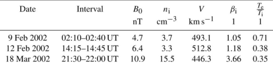
Table 1.Magnetic field magnitudeB0, ion number densityni, flow speedV, ion beta, and electron-to-ion temperature ratio for ions of the solar wind data added to that in Narita et al. (2014). Items are sorted in ascending order of ion beta.
Date Interval B0 ni V βi TTei
nT cm−3 km s−1 1 1
9 Feb 2002 02:10–02:40 UT 4.7 3.7 493.1 1.05 0.71 12 Feb 2002 14:15–14:45 UT 6.4 3.3 512.8 1.18 0.38 18 Mar 2002 21:30–22:00 UT 10.9 15.5 446.3 3.66 0.35
the azimuthal anglesφaround the mean magnetic field.
E(2-D)(k⊥, kk)= Z
dφ Z
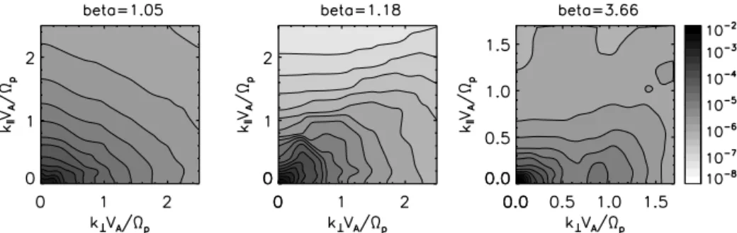
dω E(4-D)(k⊥, kk, φ, ω). (3) The perpendicular components of wavevectors therefore rep-resent the magnitude, not in any specific direction. The two-dimensional wavevector spectra for the three time intervals are displayed in Fig. 1 using the normalization to the pro-ton inertial length by multiplying VA
p (hereVA denotes the
Alfvén speed and p the proton cyclotron frequency). Ex-cept for the case at ion beta 3.66, the measured wavevector spectra are determined at the wavevector components up to
kVA
p =2.5. At ion beta 3.66, the spectrum was determined up
to kVA
p =1.7.
The wavevector anisotropy is then evaluated in the reduced spectra using the method of anisotropy index (Eq. 2). The lower limit and the higher limit of the wavenumbers are set to
kVA
p =0.3 and
kVA
p =2.5, respectively, in the computation of
anisotropy index. The lower limit is determined such that the pump waves set in the simulation work (see below) are not counted as anisotropy (the pump waves have the wavenum-bers up to kVA
p =0.2). The upper limit is determined such
that all intervals (except for ion beta 3.66) have the same range in the wavenumbers. At ion beta 3.66, we use the up-per limit kVA
p =1.7. For error estimate of the anisotropy
in-dex, these wavenumbers are varied by 10 % and this effect is transmitted to computation of the index. The anisotropy profile as a function of ion beta is displayed in Fig. 6 in the following section.
2.2 Direct numerical simulation
Direct numerical simulation serves as an independent and complementary approach of the anisotropy study. The wavevector anisotropy is studied under six different condi-tions of ion beta (0.05, 0.1, 0.2, 0.5, 1.0, and 2.0) cover-ing nearly 2 orders of magnitude. Followcover-ing the procedure in the observational approach, the wavevector spectra are deter-mined from the numerical simulation of plasma turbulence, and the anisotropy is evaluated using the spectra. However, due to the computational load, we have to limit ourselves to the two-dimensional space spanned by the parallel and the perpendicular directions to the large-scale magnetic field.
In this setup, eddies which are intrinsic to fluid-mechanical or gas-dynamic nature of plasmas are suppressed due the lack of the degree of freedom around the large-scale mag-netic field. In other words, though the spatial dimensions are two, this numerical setup is advantageous in studying the wave dynamics of plasmas in detail without being influenced by eddies.
Turbulence is produced in the simulation box by solving dynamics of plasma and fields in a step-by-step fashion. We use the hybrid plasma code AIKEF (Adaptive Ion Kinetic Electron Fluid). This code solves a set of Newtonian equation of motion for ions as super-particles under the Coulomb and Lorenz forces together with the Maxwell equations. Elec-trons are treated as a massless charge-neutralizing fluid (see details on the code in Müller et al., 2011). In contrast to the analytic approach of solving plasma dynamics, the simula-tion approach requires neither a priori knowledge on the sta-tistical property such as a Gaussian distribution of the fluctu-ating fields nor an assumption of the wave modes. The hybrid plasma treatment is suitable particularly for resolving ion ki-netic effects as far as electron gyro-motion can be neglected, i.e., on the spatial scales between the electron and ion gy-roradii (cf. 10–100 km in the solar wind). A disadvantage is that the strong electrostatic effects due to charge localiza-tion cannot develop due to the massless electron fluid, as the electrostatic field is immediately canceled out by electrons. However, the charge localization can safely be neglected in our purpose of anisotropy study here.
Implementation of the AIKEF code to our simulation study follows that presented by Verscharen et al. (2012), Comi¸sel et al. (2013) and NCM14. The simulation box has the size 250×250 proton inertial lengths, and is spanned by the parallel to the large-scale magnetic fieldB0(thez direc-tion) and the perpendicular direction (they direction). The large-scale field is constant in space and time. The spatial configuration is two-dimensional, but the vectorial quanti-ties are treated as three-dimensional, e.g., fluctuating mag-netic field, electric field, particle velocities. Thex direction is pointing out of the simulation plane. Plasma is modeled as the electron–proton plasma.
As the initial condition, a superposition of 1000 Alfvén waves with random initial phases are set to the system. These pump waves are limited to the wavevectors in the range kminVA
p =0.05 and
kmaxVA
Figure 1.Magnetic energy spectra in the plane spanned by the perpendicular and parallel components of the wavevectors with respect to the large-scale magnetic field measured by Cluster spacecraft in the solar wind.
of plasma is valid. Wavevectors are randomly and isotropi-cally chosen. The amplitude of the pump waves follows Kol-mogorov’s inertial-range scaling for fluid turbulence; that is, the spectral energy density is set to proportional to|k|−5/3. In addition, the total fluctuation amplitude is set to 1 % of the large-scale magnetic field, δBB
0 =0.01. To generate the
magnetohydrodynamic Alfvén waves, the plasma velocity is set to correlated to the pump wave magnetic field at the initial time. The periodic boundaries are set to the simula-tion. No fluctuation energy is given externally into the sys-tem, neither the fluid-scale range (kVA
p <1) nor the kinetic
range (kVA
p >1) during the simulation. Thus, fluctuations (or
waves) in the ion-kinetic domain evolve as a consequence of large-scale Alfvén waves.
The simulation box is divided into 1024×1024 compu-tational cells. The number of super-particlesN per cell are spanning in the range from N=400 to N=1600 per cell while the ion beta values are in the range between 0.05 and 2.0. We note that the higher value of ion beta one uses in the simulation, the more particles need to be put into the sim-ulation box. Otherwise many particles may leave the com-putation cell due to their thermal mobility in the high-beta plasma. This process will eventually lead to a failure in solv-ing the equations of the electromagnetic field when the so-called vacuum cell is formed in which no ion is stored in-stantaneously. To carry out a successful run at the value of ion beta 2.0, a large number of super-particles is set,N=1600, which is a highly demanding computation.
The wavevector spectra are determined at 2000 ion gy-roperiods (t p=2000) or even at later times, by extending the iterations in the simulation run (cf. anisotropy study in NCM14 uses the evolution time at t p=1000) or by in-troducing new runs. This represents a long simulation run for plasma turbulence using AIKEF code, and the fluctua-tions reach a quasi-stationary stage at which the fluctuation amplitude, the spectrum, and the anisotropy do not evolve substantially any more. The spectra are obtained by applying the fast Fourier transform algorithm to the spatial distribu-tion of magnetic field fluctuadistribu-tions (Fig. 2). New runs have been additionally carried out in order to evaluate the range
of variation of the anisotropy with respect to some simula-tion parameters, e.g., grid grid resolusimula-tion or the number of super-particles. The perpendicular wavevector components in the two-dimensional spectra for the simulation data are chosen in the direction perpendicular to the mean magnetic field within the simulation plane. Again, the anisotropy in-dex is computed at each value of ion beta using Eq. (2). In the next section, the anisotropy–time evolution is shown in Figs. 3, 4, and 5, while the anisotropy–beta relation is dis-played in Figs. 6 and 7.
3 Results and discussion 3.1 Two-dimensional spectra
The added solar wind intervals of the Cluster measurements show a diversity (including both similarities and differences) in the contour shapes of the wavevector spectra. First of all, all the three cases exhibit the anisotropy that the spec-trum is extended primarily in the direction perpendicular to the large-scale magnetic field. That is, the spectral de-cay in the wavevector domain is flatter along the perpendic-ular wavevector axis, while it is steeper along the parallel wavevector axis. A closer look at the spectra yields the fol-lowing detailed structures. In the case of ion beta 1.05 (left panel in Fig. 1), the contours of the spectrum are nearly di-agonal, connecting a larger value of the parallel component of wavevector to a larger value of the perpendicular one. In the case of ion beta 1.18, the spectral extension appears not only in the perpendicular direction but also in oblique direc-tion (about 60◦from the direction of the large-scale magnetic field). While these two cases show the monotonous spectral decay toward larger values of the wavevector components, the spectrum in the case of ion beta 3.66 exhibits a formation of the secondary peak along the perpendicular wavevector axis at about k⊥VA
p =0.8 and the third peak in the oblique
direction at about(k⊥VA
p ,
kkVA
p )=(1.6,1.2). The spectral
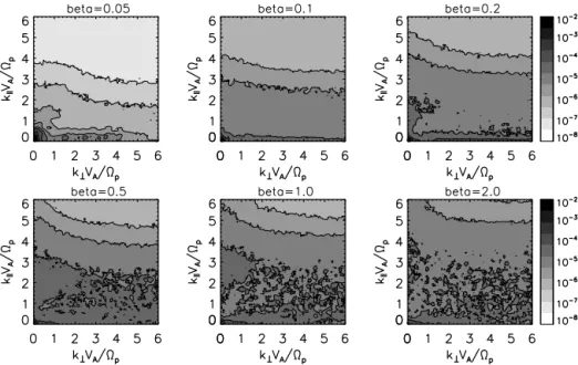
Figure 2.Magnetic energy spectra obtained by numerical simulation of two-dimensional ion-scale plasma turbulence at a late-stage time evolution (2000 ion gyroperiods). The panel styles are the same as those in Fig. 1
Figure 3. Anisotropy evolution for the data obtained by nu-merical simulation in a broad range of wavenumbers (0.3<
kVA
p <6) at the values of ion beta (from top to bottom) βi=
{0.05,0.1,0.2,0.5,1,2}.
shapes. Again, the primary extension of the spectrum ap-pears along the perpendicular wavevector direction (the spec-tral decay is flatter in the perpendicular direction, and steeper in the parallel direction). Still, the secondary peak is formed along the parallel wavevector axis (e.g., 1<kkVA
p <2 at ion
beta 0.2, 2<kkVA
p <3.5 at ion beta 1.0). It is also
inter-esting to note that the contour shape at smaller values of the perpendicular wavevector component exhibits a similar-ity in that there is a hump or a spectral extension, e.g., the transitions from (k⊥VA
p ,
kkVA
p )=(0.5,2.8) at ion beta 0.05
to (k⊥VA
p ,
kkVA
p )=(0.5,4.0) at ion beta 0.2, and further to
(k⊥VA
p ,
kkVA
p )=(0.5,5.0)at ion beta 0.5. In contrast, at larger
values of the perpendicular wavevector component, the spec-tral contours do not vary across the parallel wavevector com-ponent.
Figure 4.Anisotropy evolution for the data obtained by numeri-cal simulation at the values of ion betaβi= {0.05,0.1,0.2}in the wavenumber range 0<kVA
p <3.
Figure 5.Anisotropy evolution for the data obtained by numerical simulation at the values of ion betaβi= {0.5,1,2}in the wavenum-ber range 0<kVA
3.2 Anisotropy evolution
The anisotropy index was initially determined from simula-tion in the wavenumber range 0.3<kVA
p <6. The obtained
anisotropy is plotted as a function of time in Fig. 3. After the sudden increase at the earliest time, the anisotropy index reaches a saturation level in fewer than 15 ion gyroperiods without crossing the evolution curves at the other values of ion beta throughout the simulation runs until 2000 ion gy-roperiods. The exception is the case at the smallest value of ion beta (βi=0.05) that the anisotropy index increases and peaks at about 500 ion gyroperiods, and then decreases. The beta dependence that the anisotropy is reduced with increas-ing ion beta can been seen even in the early evolution phase around a few ion gyroperiods. Furthermore, the anisotropy index at ion beta 0.05 turns back at later times (t p>1500). Whether this peculiar evolution is due to the thermal fluc-tuations (see, e.g., Yoon et al., 2014) or due to the numeri-cal noise of the hybrid particle-in-cell (PIC) simulation (see, e.g., Jenkins and Lee , 2007) is a question we cannot answer in this paper. Nevertheless, there is no connection with the initial Alfvénic excitation imposed at the start of the simula-tion.
We found that the fast saturation of the anisotropy at the initial time is a consequence of the contribution of high wavenumber terms of the power spectrum. By using a low-pass filter in the fluctuating magnetic field, the quick satu-ration of the anisotropy at the initial time is removed. The higher the ion beta value is, the lower the cutoff wavenumber (kcut) has to be employed. The effect of filtering the fluctu-ating magnetic field spectrum is demonstrated in Fig. 4 for ion beta 0.05, 0.1, 0.2, and in Fig. 5 for ion beta 0.5, 1, and 2. The cutoff wavenumber was kcutVAp =3 andkcutVAp =1, respectively.
The anisotropy index starts to increase abruptly and at-tends a peak value aroundt p≈500 at ion beta 0.05 while for ion beta 0.1 and 0.2 the growing is slow and the crests are at t p≈1000 and t p≈1700, respectively. At larger ion beta values, the anisotropy index evolves smoothly and extends to a saturation level after time 500 ion gyroperiods. The anisotropy index decreases with the increase of ion beta as in the previous evaluation except ion beta 0.5.
The reduced anisotropy with increasing beta was already pointed out from the particle-in-cell simulations (Chang et al., 2013) for whistler turbulence on electron kinetic scales. Our result confirms this tendency even on the ion kinetic scales. We note however that the peaks of the anisotropy at the low ion beta values evolve differently than those from Chang et al. (2013). In our plots (Fig. 4), the peak is achieved more quickly at lower ion beta values, while in the PIC simu-lation a reversed dependence with electron beta is observed.
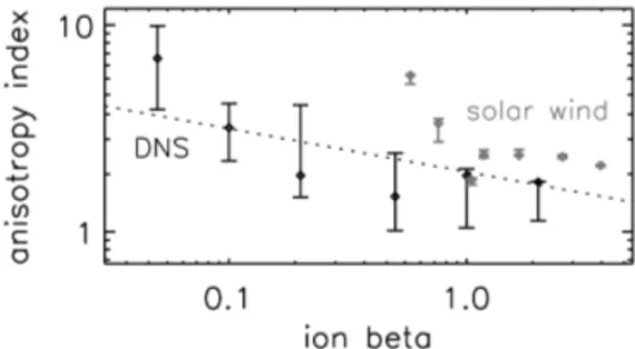
Figure 6.Ion beta dependence of anisotropy index obtained by the Cluster spacecraft measurements in the solar wind (in gray) and that by direct numerical simulation (DNS, in black) with the power-law fitting.
3.3 Search for anisotropy scaling
The experimental anisotropy index is plotted as a function of ion beta at once with the latter values obtained from simula-tion (filtered data) in Fig. 6. The evaluated anisotropy index from Cluster measurements is about 1.8 (at ion beta 1.05), 2.3 (at ion beta 1.18), and 2.1 (at ion beta 3.66). These val-ues are plotted in Fig. 6 together with those already obtained in NCM14 (5.7 at ion beta 0.58, 3.3 at ion beta 0.76, 2.3 at ion beta 1.66, and 2.3 at ion beta 2.53). The results from simulation were obtained by averaging the time-dependent anisotropies shown in Figs. 4 and 5 as 6.9 (at ion beta 0.05), 3.2 (at ion beta 0.1), 1.9 (at ion beta 0.2), 1.5 (at ion beta 0.5), 1.9 (at ion beta 1.0), and 1.7 (at ion beta 2.0).
Both the spacecraft measurements and the numerical sim-ulations show that the anisotropy is stronger (i.e., the spectral decay is steeper along the parallel wavevector axis) when ion beta is below unity, and is moderate and asymptotes slowly to isotropy (A→1) when ion beta is above unity. However, the quantitative picture of the beta dependence is different between the observations and the simulations. In the space-craft measurements in the solar wind, the anisotropy index falls down rather abruptly in the range of ion beta from 0.5 to 1, and then forms a plateau with only moderate decrease in the anisotropy index. Furthermore, the anisotropy index measured in the solar wind tends to be higher than that from the simulations. In the simulation, the anisotropy falls down more steeply at low ion beta (at 0.05, 0.1 and 0.2) and then decreases smoothly at higherβi (1, 2). This is similar to the tendency observed in the solar wind if the shift in ion beta is disregarded.
The beta dependence of the anisotropy determined from the unfiltered data is given separately in Fig. 7. It clearly shows a monotonic descending trend that exhibits a power-law scaling in the formA∝βi−α. The slope in the scaling can be determined by the fitting procedure, and we obtain the empirical scaling
Figure 7.Ion beta dependence of anisotropy index from Fig. 3 and the power-law fitting.
Figure 8.Anisotropy index plotted as a function of electron-to-ion temperature ratio as measured by the Cluster spacecraft in the solar wind.
Equation (4) represents with small deviations the anisotropy index controlled by the thermal or by the hybrid PIC sim-ulation noise. Dieckmann et al. (2004) studied the noise spectra of electrostatic waves in an unmagnetized electron plasma by PIC simulations. The purpose of their work was to find out the interplay between three categories of noise: thermal, numerical and PIC simulation noise. Their results show that at smaller wavenumbers the estimated numerical noise dominates the simulation noise, while at large values near the Nyquist wavenumber, the thermal noise becomes more effective. We repeated the simulations for short times (t p<200) by varying the number of super-particles, and therefore, by changing the numerical noise amplitude, an-other set of anisotropy indices was determined. An addi-tional anisotropy index extends our study at higher values of ion beta (βi=4). This numerical experiment shows evi-dence that the anisotropy power-law scaling from Eq. (4) is linked to thermal rather than to numerical noise. The power-law dependence is added in Fig. 6. The anisotropy index of the simulated turbulent cascade follows the power law in the limit of the error bars.
For the spacecraft measurements, two additional tests for possible relation with the wavevector anisotropy have been conducted: (1) effect of the electron-to-ion temperature ra-tio and (2) effect of the magnetic field magnitude. Figure 8 shows the plot of the anisotropy as a function of the
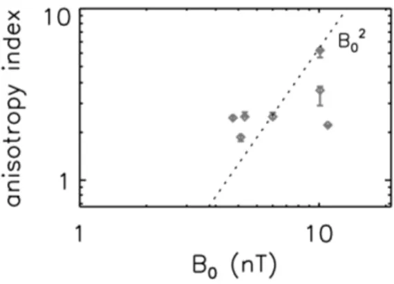
temper-Figure 9.Anisotropy index plotted as a function of the mean mag-netic field magnitude as measured by the Cluster spacecraft in the solar wind. The dotted line is a scaling law (Eq. 5) predicted by Dastgeer and Zank (2003) for electron magnetohydrodynamic tur-bulence.
ature ratio derived from the Cluster spacecraft measurements (for the test 1). Data set includes that used in our previous pa-per (NCM14). Due to large variation of anisotropy around the temperature ratio about 0.35, no clear trend or organization can be confirmed about the possible relationship between the anisotropy and the temperature ratio. However, the data point at the smallest anisotropy value at (Te/Ti, A)≃(0.7,1.8) could be a sign of the temperature-ratio dependence as in-dicated by Valentini et al. (2010).
Figure 9 shows the plot of the anisotropy index as a func-tion of the mean magnetic field magnitude derived from the Cluster data analysis (for the test 2). There is a weak ten-dency that the anisotropy is stronger with increasing mag-netic field magnitude. In electron magnetohydrodynamics it is known that anisotropy depends on the strength of large-scale magnetic field (Dastgeer and Zank, 2003) as
A∝B02. (5)
In their paper, the anisotropy quantity (the symbol R was used) is related to our definition of the anisotropy index by
R=A−2. This scaling is verified using our anisotropy mea-surements using Cluster spacecraft data. Comparison with the numerical simulation data is not possible here, since the magnetic field is normalized to unity and the thermal pres-sure is varied in the simulations. The meapres-sured slope shows the same tendency as that derived by Dastgeer and Zank (2003), but it is flatter than the scalingB02. We interpret that the dependence of anisotropy on ion beta comes partly from the magnetic field magnitude and partly from the plasma thermal pressure.
4 Conclusions
wavevector anisotropy of plasma turbulence at ion-scale wavelengths becomes weaker with increasingβi.
This fact, however, should not be taken as surprising when considering that the role of magnetic field is weaker in high-beta plasmas. We observe the primary extension of the wavevector spectrum in the perpendicular direction to the large-scale magnetic field, which supports the notion of fila-mentation process in structure formation.
Furthermore, our two-dimensional hybrid simulations show that a power-law scaling relation between the wavevec-tor anisotropy and βi could exist. The power-law function was found to describe accurately the anisotropy index driven by the thermal or hybrid PIC simulation noise. What deter-mines the scaling slopeα≃0.3 will be a subject of theoreti-cal and computational studies.
It may be worth while to compare with the other observa-tional fact that the variance anisotropy (which is a measure of compressibility in magnetic field fluctuations) also exhibits a power-law scaling to ion beta with the slope−0.56 (Smith et al., 2006).
We point out that the logic in our work can be reversed; that is, the scaling law can be applied to measurements of magnetic field as a diagnostic tool of ion beta. At the current stage, such a method is applicable in two-dimensional plas-mas. Still, the method can be used to constrain the value of ion beta in three-dimensional plasmas as well. An interesting extension would be an application to astrophysical systems. If such a scaling existed in the magnetohydrodynamic pic-ture of plasmas, one could obtain or constrain the value of ion beta by analyzing photometry data of filament structures in interstellar media or astrophysical jets.
Author contributions. H. Comi¸sel: Simulation, analysis, writing. Y. Narita: Observation, analysis, writing. U. Motschmann: Coor-dination, interpretation.
Acknowledgements. H. Comi¸sel acknowledges Daniel Verscharen for comments and suggestions. This is financially supported by Collaborative Research Center 963,Astrophysical Flow, Instabili-ties, and Turbulence of the German Science Foundation and FP7 313038 STORM of European Commission. We also acknowledge North-German Supercomputing Alliance (Norddeutscher Verbund zur Förderung des Hoch- und Höchstleistungsrechnens – HLRN) for supporting direct numerical simulations.
Edited by: J. Büchner
Reviewed by: two anonymous referees
References
Ahlers, M.: Anomalous anisotropies of cosmic rays from turbulent magnetic fields, Phys. Rev. Lett., 112, 021101, doi:10.1103/PhysRevLett.112.021101, 2014.
Balogh, A., Carr, C. M., Acuña, M. H., Dunlop, M. W., Beek, T. J., Brown, P., Fornaçon, K.-H., Georgescu, E., Glassmeier, K.-H., Harris, J., Musmannn, G., Oddy, T., and Schwingenschuh, K.: The Cluster magnetic field investigation: overview of in-flight performance and initial results. Ann. Geophys., 19, 1207–1217, doi:10.5194/angeo-19-1207-2001, 2001.
Bieber, J. W., Matthaeus, W. H., Smith, C. W., Wanner, W., Kallen-rode, M.-B., and Wibberenz, G.: Proton and electron mean free paths: The Palmer consensus revisited, Astrophys. J., 420, 294–306, doi:10.1086/173559, 1994.
Bieber, J. W., Wanner, W., and Matthaeus, W. H.: Dominant two-dimensional solar wind turbulence with implications for cosmic ray transport, J. Geophys. Res., 101, 2511–2522, doi:10.1029/95JA02588, 1996.
Chang, O., Gary, S. P., and Wang, J.: Whistler turbulence at variable electron beta: Three-dimensional particle-in-cell sim-ulations, J. Geophys. Res. Space Phys., 118, 2824–2833, doi:10.1002/jgra.50365, 2013.
Chen, C. H. K., Mallet, A., Schekochihin, A. A., Horbury, T. S., Wicks, R. T., and Bale S. D.: Three-dimensional struc-ture of solar wind turbulence, Astrophys. J., 758, 120, 5 pp., doi:10.1088/0004-637X/758/2/120, 2012.
Choi, J., Song, I., and Kim, H. M.: On estimating the direction of ar-rival when the number of signal sources is unknown, Signal Pro-cess, 34, 193–205, doi:10.1016/0165-1684(93)90162-4, 1993. Comi¸sel, H., Verscharen, D., Narita, Y., and Motschmann, U.:
Spec-tral evolution of two-dimensional kinetic plasma turbulence in the wavenumber-frequency domain, Phys. Plasmas, 20, 090701, doi:10.1063/1.4820936, 2013.
Cumming, A., Arras, P., and Zweibel, E.: Magnetic field evolution in neutron star crusts due to the Hall effect and Ohmic decay, Astrophys. J., 609, 999–1017, doi:10.1086/421324, 2004. Dasso, S., Milano, L. J., Matthaeus, W. H., and Smith, C. W.:
Anisotropy in fast and slow solar wind fluctuations, Astrophys. J., 635, L181–L184, doi:10.1086/499559, 2005.
Dastgeer, S. and Zank, G. P.: Anisotropic turbulence in two-dimensional electron magnetohydrodynamics, Astrophys. J., 599, 715–722, doi:10.1086/379225, 2003.
Dieckmann, M. E., Ynnerman, A., Chapman, S. C, Rowlands, G., and Andersson, N.: Simulating thermal noise, Physica Scripta, 69, 456–460, doi:10.1238/Physica.Regular.069a00456, 2004. Drake, D. J., Schroeder, J. W. R., Howes, G. G., Kletzing, C. A.,
Skiff, F., Carter, T. A., and Auerbach, D. W.: Alfvén wave collisions, the fundamental building block of plasma turbu-lence. IV. Laboratory experiment, Phys. Plasmas, 20, 072901, doi:10.1063/1.4813242, 2013.
Gary, S. P., Saito, S., and Narita, Y.: Whistler turbulence wavevec-tor anisotropies: particle-in-cell simulations, Astrophys. J., 716, 1332–1335, doi:10.1088/0004-637X/716/2/1332, 2010. Howes, G. G., Tenbarge, J. M., Dorland, W., Quataert, E.,
Howes, G. G., Drake, D. J., Nielson, K. D., Carter, T. A., Kletzing, C. A., and Skiff, F.: Toward astrophysical tur-bulence in the laboratory, Phys. Rev. Lett., 109, 255001, doi:10.1103/PhysRevLett.109.255001, 2012.
Jenkins, T. G. and Lee, W. W.: Fluctuations of discrete particle noise in gyrokinetic simulation of drift waves, Phys. Plasmas, 14, 032307, doi:10.1063/1.2710808, 2007.
Matthaeus, W. H., Goldstein, M. L., and Roberts, D. A.: Evi-dence for the presence of quasi-two-dimensional nearly incom-pressible fluctuations in the solar wind, J. Geophys. Res., 95, 20673–20683, doi:10.1029/JA095iA12p20673,1990.
Matthaeus, W. H., Gosh, S., Ougton, S., and Roberts, D. A.: Anisotropic three-dimensional MHD turbulence, J. Geophys. Res., 101, 7619–7630, doi:10.1029/95JA03830, 1996.
Matthaeus, W. H. and Gosh, S.: Spectral decomposition of solar wind turbulence: Three-component model, AIP Conf. Proc. The solar wind nine conference, 5–9 October 1998, Nantucket, Mas-sachusetts, 471, 519–522, doi:10.1063/1.58688, 1999.
Müller, J., Simon, S., Motschmann, U., Schüle, J., Glassmeier, K.-H., and Pringle, G. J.: Adaptive hybrid model for space plasma simulations, Comp. Phys. Comm., 182, 946–966, doi:10.1016/j.cpc.2010.12.033, 2011.
Narita, Y. and Glassmeier, K.-H.: Anisotropy evolution of magnetic field fluctuation through the bow shock, Earth Planet. Space, 62, e1–e4, doi:10.5047/eps.2010.02.001, 2010.
Narita, Y., Glassmeier, K.-H., and Motschmann, U.: High-resolution wave number spectrum using multi-point measure-ments in space – the Multi-point Signal Resonator (MSR) tech-nique, Ann. Geophys., 29, 351–360, doi:10.5194/angeo-29-351-2011, 2011.
Narita, Y., Comi¸sel, H., and Motschmann, U.; Spatial struc-ture of ion-scale plasma turbulence, Front. Phys., 2, 13, doi:10.3389/fphy.2014.00013, 2014.
Rème, H., Aoustin, C., Bosqued, J. M., Dandouras, I., Lavraud, B., Sauvaud, J. A., Barthe, A., Bouyssou, J., Camus, Th., Coeur-Joly, O., Cros, A., Cuvilo, J., Ducay, F., Garbarowitz, Y., Medale, J. L., Penou, E., Perrier, H., Romefort, D., Rouzaud, J., Vallat, C., Alcaydé, D., Jacquey, C., Mazelle, C., d’Uston, C., Möbius, E., Kistler, L. M., Crocker, K., Granoff, M., Mouikis, C., Popecki, M., Vosbury, M., Klecker, B., Hovestadt, D., Kucharek, H., Kuenneth, E., Paschmann, G., Scholer, M., Sckopke, N., Seiden-schwang, E., Carlson, C. W., Curtis, D. W., Ingraham, C., Lin, R. P., McFadden, J. P., Parks, G. K., Phan, T., Formisano, V., Amata, E., Bavassano-Cattaneo, M. B., Baldetti, P., Bruno, R., Chion-chio, G., Di Lellis, A., Marcucci, M. F., Pallocchia, G., Korth, A., Daly, P. W., Graeve, B., Rosenbauer, H., Vasyliunas, V., Mc-Carthy, M., Wilber, M., Eliasson, L., Lundin, R., Olsen, S., Shel-ley, E. G., Fuselier, S., Ghielmetti, A. G., Lennartsson, W., Es-coubet, C. P., Balsiger, H., Friedel, R., Cao, J.-B., Kovrazhkin, R. A., Papamastorakis, I., Pellat, R., Scudder, J., and Sonnerup, B.: First multispacecraft ion measurements in and near the Earth’s magnetosphere with the identical Cluster ion spectrometry (CIS) experiment, Ann. Geophys., 19, 1303–1354, doi:10.5194/angeo-19-1303-2001, 2001.
Saito, S., Gary, S. P., Li, H., and Narita, Y.: Whistler turbu-lence: Particle-in-cell simulations, Phys. Plasmas, 15, 102305, doi:10.1063/1.2997339, 2008.
Saito, S., Gary, S. P., and Narita, Y.: Wavenumber spectrum of whistler turbulence: Particle-in-cell simulation, Phys. Plasmas, 17, 122316, doi:10.1063/1.3526602, 2010.
Saito, S. and Gary, S. P.: Beta dependence of electron heating in decaying whistler turbulence: Particle-in-cell simulations, Phys. Plasmas, 19, 012312, doi:10.1063/1.3676155, 2012.
Schmidt, R. O.: Multiple emitter location and signal param-eter estimation, IEEE Trans. Ant. Prop., AP-34, 276–280, doi:10.1109/TAP.1986.1143830, 1986.
Shebalin, J. V., Matthaeus, W. H., and Montgomery, D.: Anisotropy in MHD turbulence due to a mean magnetic field, J. Plasma Phys., 29, 525–547, doi:10.1017/S0022377800000933, 1983. Smith, C. W., Vasquez, B. J., and Hamilton, K.: Interplanetary
mag-netic fluctuation anisotropy in the inertial range, J. Geophys. Res., 111, A09111, doi:10.1029/2006JA011651, 2006.
Valentini, F., Califano, F., and Veltri, P.: Two-dimensional kinetic turbulence in the solar wind, Phys. Rev. Lett., 104, 205002, doi:10.1103/PhysRevLett.104.205002, 2010.
Verscharen, D., Marsch, E., Motschmann, U., and Müller, J.: Ki-netic cascade beyond magnetohydrodynamics of solar wind tur-bulence in two-dimensional hybrid simulations, Phys. Plasmas, 19, 022305, doi:10.1063/1.3682960, 2012.