ISSN 1549-3644
© 2009 Science Publications
On the Pseudo-Spectral Method of Solving Linear Ordinary
Differential Equations
B.S. Ogundare
Department of Pure and Applied Mathematics,
University of Fort Hare, Alice 5700 RSA
Abstract: Problem statement: Not all differential equations can be solved analytically, to overcome
this problem, there is need to search for an accurate approximate solution. Approach: The objective of this study was to find an accurate approximation technique (scheme) for solving linear differential equations. By exploiting the Trigonometric identity property of the Chebyshev polynomial, we developed a numerical scheme referred to as the pseudo-pseudo-spectral method. Results: With the scheme developed, we were able to obtain approximate solution for certain linear differential equations. Conclusion: The numerical scheme developed in this study competes favorably with solutions obtained with standard and well known spectral methods. We presented numerical examples to validate our results and claim.
Key words: Chebyshev polynomial, linear ordinary differential equations, Spectral method,
Pseudo-spectral method, pseudo-pseudo-Pseudo-spectral method.
INTRODUCTION
The fundamental problem of approximation of a function by interpolation on an interval paved way for the spectral methods which are found to be successful for the numerical solution of ordinary and partial differential equations. Spectral representations of analytic studies of differential equations have been in used since the days of Fourier. Their application to Numerical solution of ordinary differential equations refers, at least to the time of Lanczos[10]. Summary of survey of some applications is given in[8]. Some present spectral methods can also be traced back to the "'method of weighted residuals"' of Finlayson and Scriven[6].
Spectral methods can be viewed as an extreme development of the class of discretization scheme for differential equations known as the Method of Weighted Residuals (MWR)[6]. In MWR, the use of approximating functions (called trial functions) is central. These functions are used as basis functions for a truncated series expansion of the solution. Another function called the test functions (also known as the weight functions) are used to ensure that the differential equation is satisfied as close as possible by the truncated series expansion. Among the spectral schemes the three most commonly used are the Tau, Galerkin and collocation (also called pseudo-spectral) methods. What distinguishes between these methods is the choice of the test functions employed. Galerkin and
Tau method are implemented in terms of the expansion coefficients[5], whereas collocation methods are implemented in terms of physical space values of unknown function. Over the past two decades, spectral methods with their current forms appeared as attractive ways in most applications. Some more details on spectral methods could be seen in[9,11-13].
The basic idea of spectral methods to solve differential equations is to expand the solution function as a finite series of very smooth basis functions, as given below:
N
k k k 0
y(x) a (x)
=
=
∑
φ (1)where, φ represents Chebyshev or Legendre polynomials[14] (for more on Chebyshev polynomials). If y∈C∞a, b, the error produced by the approximation approaches zero with exponential rate[4] as N becomes too large (tends to infinity). This phenomenon is referred to as 'spectral accuracy[8]. The accuracy of the derivative obtained by direct term-by-term differentiation of such truncated expansion naturally deteriorates[4], but for low-order derivatives and sufficiently high-order truncations this deterioration is negligible, compared to the restrictions in accuracy introduced by typical difference approximations.
solution function is not analytic on the interval of definition. Weak aspect of spectral methods in solving this kind of problems were studied in[2] and[3] and the researchers came up with modifications to the spectral method which proved to be more efficient when compared with existing ones.
In this article, we present a variation of the collocation (pseudo-spectral) method to solve the problems of[2] and[3]. The pseudo-pseudo-spectral method (the method introduced in this article) is seen to be efficient and competes favorable with other well-known standard methods like the Tau method, Galerkin Method and the Pseudo-spectral (collocation) method.
MATERIALS AND METHODS
Pseudo-pseudo-spectral method: Consider the
following differential equation: m
i m i i 0
Ly f −(x)D y f (x), x a, b
=
=
∑
= ∈ (2)Ty = K (3)
where, fi, i = 0,1,…m f, are known functions of x, Di is the order of differentiation with respect to the independent variable x, T is a linear functional of rank
N and m
K∈ .
Here (3) can either be initial, boundary or mixed conditions. To solve the above class of equations using the spectral method is to expand the solution function y, in (2) and (3) as a finite series of very smooth functions in the form below:
N N
k k k 0
y (x) a T (x)
=
=
∑
(4)where,
{
k}
0T (x) ∞ is the sequence of Chebyshev
polynomials of the first kind. Replacing y by yN in (3) the residual is defined as:
N N
r (x)=Ly −f (5)
The main target and objective in spectral method is to minimize rN as much as possible with regard to (3). The implementation of the spectral methods leads to a system of linear equations with N+1 equations in N+1 unknowns a0,a1,…,aN
Here we present a variation (pseudo) of one of the three spectral methods called collocation (also known as pseudo-spectral) method. We call this method a pseudo-pseudo-spectral method. Also, we use both the
Tau and the pseudo-spectral methods for numerical solution of second order linear differential equations to compare the result with pseudo-pseudo-spectral method.
We need to state here that this discussion can be extended to the general problem of the form (2) and (3). Consider the following differential equation:
'' '
P(x)y (x) Q(x)y (x) R(x)y(x) S(x), x [ 1,1]
y( 1) , y(1)
+ + = ∈ −
− = α = β (6)
With the pseudo-pseudo-spectral method, we suppose that the approximate solution of the Eq. 6 is given by:
N
N '
k k k 0
y (x) a T (x)
=
=
∑
(7)instead of (4) for an arbitrary natural number N, where T N 1
0 1 N
a=(a ,a ,...,a ) ∈ + is the constant coefficients vector and
{
T (x)k}
0∞
is the sequence of Chebyshev polynomials of the first kind. The prime denotes that the first term in the expansion is halved.
In this method, as against the use of a function V(x) as in the standard Tau method and the Pseudo-spectral method[2,3,7], we instead of using the Chebyshev polynomial as a polynomial we exploit the trigonometric property of Chebyshev function.
Let: N
' k k k 0
y(x) a T (x)
=
=
∑
(8)be the approximate solution for the Eq. 6, as a solution it must satisfy the equation.
Recall the definition of a Chebyshev polynomial: 1
k
T (x)=cos(k cos (x))−
Let:
1
cos x,− x cos
θ = ⇒ = θ
Then:
k k
T (x)=T ( )θ =cos kθ
Using the identity defined above, (8) becomes: N
' k k 0
y(x) a cos k
=
The first and second derivatives of (9) are respectively given as:
N
' k k 0
k sin k
y '(x) a ( )
sin = θ = θ
∑
(10) 2 N ' k 3 k 0k sin k cos k cos k sin
y ''(x) a ( )
sin
=
θ θ − θ θ
=
θ
∑
(11)Substituting (9-11) into the equation (6) with the functions P, Q, R and S expressed in terms of θ we have: 2 N ' k 3 k 0 N ' k k 0 N ' k k 0
k sin k cos k cos k sin
P( ) a
sin
k sin k
Q( ) a
sin
R( ) a cos S( ) , ,
y( ) , y( )
=
=
=
θ θ − θ θ
θ
θ
θ
+ θ θ
+ θ θ = θ θ∈ −π π
−π = α π = β
∑
∑
∑
(12) N ' k k k 0a ( ) S( )
=
φ θ = θ
∑
(13)Simplifying Eq. 11, we have:
2 N
'
k k 3
k 0
N N
' '
k k
k 0 k 0
k sin k cos k cos k sin
( ) P( ) a
sin
k sin k
Q( ) a R( ) a cos
sin
=
= =
θ θ − θ θ
φ θ = θ
θ
θ
+ θ θ + θ θ
∑
∑
∑
(14)
If we impose the associated conditions on (14), we have:
N N
' ' k
k k k
k 0 k 0
N N
' ' k
k k k
k 0 k 0
y( 1) a T ( 1) a ( 1)
y(1) a T (1) a (1)
= =
= =
− = α ⇒ − = − = α
= β ⇒ = = β
∑
∑
∑
∑
So: 0 1 N 2 N a a 1 a1 1 . . . ( 1) 2
. 1
1 1 . . . 1 .
2 . a − −
α
= β (15)
Relation (15) form a system with two equations and N+1 unknowns, to construct the remaining N-1 equations we Collocate (13) at the zeros of TN-1(x), which are the interior points between -1 and 1 and are given as k
(2k 1)
, k 1,..., N 1
N 1 − π
θ = = −
− , which is in great
variance to the Tau Method, the Galerkin method and the Pseudo-spectral method.
The system obtained here solves for the coefficients.
RESULTS
Here we consider some ordinary differential equations with Tau Method, Pseudo-spectral method and the Pseudo-pseudo-spectral method and present our results in Table-7.
As notations, we represent the approximations with the Tau method, Pseudo-spectral method and the Pseudo-pseudo-spectral method asy , y , yt ps pps respectively.
Numerical experiments: We shall consider the
following problems:
Problem 1:
y ''(x)+xy '(x)+ =y x cos x, y( 1)− =sin( 1),− y(1)=sin(1)
with the exact solution y(x) = sin x.
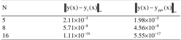
Table 1: Maximum error of approximation of problem 1
N y(x)−y (x)t ∞ y(x)−ypps(x)∞
5 2.11×10⁻⁵ 1.98×10⁻⁵ 8 5.71×10⁻⁸ 4.56×10⁻⁸ 16 1.11×10⁻¹⁶ 5.55×10⁻¹⁷
Table 2: Maximum error of approximation of problem 2
N y(x)−y (x)t ∞ y(x)−y (x)ps ∞ y(x)−ypps(x)∞
5 5×10⁻⁵ 2.09×10⁻⁵
15 2×10⁻⁶ 3.33×10⁻¹⁶
16 8×10⁻⁷ 1.67×10⁻¹⁶
18 4×10⁻¹⁹
30 5×10⁻⁷ 95 8×10⁻⁸
Table 3: Maximum error of approximation of problem 3
N y(x)−y (x)t ∞ y(x)−y (x)ps ∞ y(x)−ypps(x)∞
Table 4: Maximum error of approximation of problem 4
N y(x)−y (x)t ∞ y(x)−y (x)ps ∞ y(x)−ypps(x)∞
8 8.98×10⁻² 1.21×10⁻¹ 1.20×10⁻¹ 15 1.54×10⁻² 1.76×10⁻² 1.38×10⁻² 20 1.68×10⁻² 1.92×10⁻² 1.50×10⁻²
Table 5: Maximum error of approximation of problem 5
N y(x)−y (x)t ∞ y(x)−y (x)ps ∞ y(x) y− mps(x)∞ y(x)−ypps(x)∞
5 2.22×10⁻¹⁵ 9.09×10⁻¹⁶
8 1.63×10⁻¹⁵
9 2.53×10⁻¹⁶
12 1.38×10⁻¹⁵
17 1.25×10⁻¹⁶
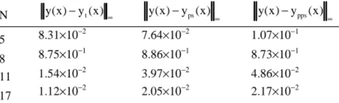
Table 6: Maximum error of approximation of problem 6
N y(x)−y (x)t ∞ y(x)−y (x)ps ∞ y(x)−ypps(x)∞
5 8.31×10⁻² 7.64×10⁻² 1.07×10⁻¹
8 8.75×10⁻¹ 8.86×10⁻¹ 8.73×10⁻¹ 11 1.54×10⁻² 3.97×10⁻² 4.86×10⁻²
17 1.12×10⁻² 2.05×10⁻² 2.17×10⁻²
Table 7: Maximum error of approximation of problem 7
N y(x)−y (x)t ∞ y(x)−y (x)ps ∞ y(x)−ypps(x)∞
5 3.26×10⁻¹ 5.99×10⁻¹ 1.84×10⁻¹ 8 2.42×10⁻¹ 9.59×10⁻¹ 2.10×10⁻² 16 2.05×10⁻¹ 5.27×10⁻¹ 7.15×10⁻²
Problem 2:
2
2
1 8
y ''(x) y '(x) , x (0,1),
x 8 x
y(1) 0,
y '(0) 0
+ = − ∈
= =
with the exact solution 2ln 7 2
8 x
−
.
Problem 3:
2 2 2 2
3 1 3 1
y ''(x) x y '(x) (x ) y(x) 1 x (x ) exp(x),
4 4
x [ 1,1], y( 1) exp( 1),
y(1) exp(1.)
+ + − = + + −
∈ − − = −
=
with the exact solution y(x) = exp(x).
Problem 4:
3 3
y ''(x) x y '(x) y(x) 6x x 3x , x [ 1,1],
y( 1) y(1) 1
+ + = + + ∈ −
− = =
with the exact solution 3
y(x)=exp(x) x .
Problem 5:
3 2
1 1
y ''(x) exp( )y '(x) 6x x 3x e xp( ),
x x
x [ 1,1], y( 1) 1,
y(1) 1
+ = + +
∈ − − = −
=
with the exact solution y(x) = x3.
Problem 6:
1 1
y ''(x) y '(x) y(x) x ,
x x
y( 1) 1,
y(1) 1
− + =
− = −
=
with the exact solution y(x)=x x .
Problem 7:
1 1
y ''(x) y '(x) y(x) x ,
x x
y( 1) y(1) 1
+ + = +
− = =
with the exact solution y(x)= x .
DISCUSSION
Problem 1 was taken from[3]. This problem was solved with Runge-Kutta of different orders and a maximum error of 3.0×10⁻¹ were recorded. It was also solved with Tau method and the method described in this study with N = 5, 8, 16. The maximum error produced for these two methods for the various N is shown in the Table 1. Table 1 shows the power of spectral methods over Runge-Kutta.
Problem 3 was chosen from[2]. It was solved with the method described in this article and the error produced for various N is shown in the Table 3 with the maximum error produced when the problem was solved by the Tau method and Pseudo-spectral method of[3].
Problem 4 was taken from[3]. The problem has a non analytic solution function which makes accompany error indispensable.
We applied our method to the problem, the error produced by the method as well as the error produced when it was solved with the Tau method and Pseudo-spectral method of[3] is shown in Table 4.
Problem 5 was chosen from[3]. When the problem is solved using the Tau method and the pseudo-spectral. method in[3], the methods failed and a modified pseudo-spectral (mps) method which was the subject of the article was used to solve the problem and the maximum error produced in[3] for the problem is shown in the Table 5 with the error produced by the method of this article. This method performs better than the modified method of[3].
Problem 6 was also from[3]. We tested our method on this problem with different values of $N$, the results are shown in Table 6.
From the Table 6 it could be seen that the pseudo-pseudo-spectral method is performing considerably well in the class of spectral methods.
Problem was 7 chosen from[3]. The results for various values of N are shown in Table 7.
The results displayed in the Table 7 show the power of the pseudo-pseudo-spectral method over the Tau and the pseudo-spectral methods.
CONCLUSION
The pseudo-pseudo-spectral method of this article is seen to be efficient and competes favorable with other well-known standard methods like the Tau method, Galerkin Method and the Pseudo-spectral (collocation) methods.
One major advantage with this method is that it does not require a tedious means of evaluating the unknown coefficients of the approximating function as in other spectral methods.
The method is easy to program and require moderately less of computer time to evaluate.
It is also seen to be suitable for any class of linear differential equations with or without analytical solutions.
REFERENCES
1. Ascher, U.M., R.M. Mahheij and R.d. Russell, 1988. Numerical Solution of Boundary Value
Problem for Ordinary Differential Equations. 1st Edn., Prentice-Hall Inc., USA., ISBN: 0-13-627266-5, pp: 619.
2. Babolian, E. and M.M. Hosseini, 2002. A modified spectral method for numerical solution of ordinary differential equations with non-analytic solution. Applied Math. Comput., 132: 341-351. DOI: 10.1016/S0096-3003(01)00197-7
3. Babolian, E., M. Bromilow, R. England and M. Savari,
2007. A modification of pseudo-spectral method for solving a linear ODEs with singularity. Applied Math. Comput., 188: 1260-1266. DOI: 10.1016/j.amc.2006.10.079.
4. Canuto, C., M. Hussaini, A. Quarteroni and T. Zang,
1988. Spectral Methods in Fluid Dynamics. Springer, Berlin, ISBN: 10: 0387173714, pp: 557. 5. Delves, L.M. and J.L. Mohamed, 1985.
Computational Methods for Integral Equations. 1st Edn., Cambridge University Press, Cambridge, ISBN: 10: 0521266297, pp: 388.
6. Finlayson, A. and L.E. Scriven, 1996. The method of weighted residuals. Applied Mech. Rev., 19: 735-748. http://www.scribd.com/doc/8984439/Method-of-Weighted-Residuals
7. Fornberg, B., 1996. A Practical Guide to Pseudo-Spectral Methods. Illustrated Edn., Cambridge University Press, Cambridge, ISBN: 0521645646, pp: 242.
8. Gottlieb, D. and S. Orszag, 1977. Numerical Analysis of Spectral Methods, Theory and Applications. 6th Edn., SIAM, Philadephia, PA., ISBN: 0898710235, pp: 172.
9. E. Gourgoulhon, 2002. Introduction to Spectral Methods, 4th EU Network meeting, Palma de Mallorca, Sept. 2002.
10. Lanczos, C., 1938. Trigonometric interpolation of empirical and analytic functions, J. Math. Phys., 17: 123-199.
11. Ortiz, E.L., 1969. The tau method. SIAM. J.
Numer. Anal., 6: 480-492.
http://www.jstor.org/stable/2949509
12. Ortiz, E.L. and J.H. Freilich, 1982. Numerical solution of system of ordinary differential equations with tau method: An error analysis.
Math. Comput., 39: 467-479.
http://www.jstor.org/stable/2007325
13. Ortiz, E.L. and T. Chaves, 1968. On the numerical solution of two-point boundary value problems for linear differential equations ZAMM. J. Applied Math. Mech., 48: 415-418. DOI: 10.1002/zamm.19680480607