On direct passive microwave remote sensing of sea spray aerosol production

(1)

ACPD

14, 15363–15417, 2014

On direct passive microwave remote sensing of sea spray

aerosol production

I. B. Savelyev et al.

Title Page

Abstract Introduction

Conclusions References

Tables Figures

◭ ◮

Back Close

Full Screen / Esc

Printer-friendly Version

Interactive Discussion

Discussion

P

a

per

|

Discus

sion

P

a

per

|

Discussion

P

a

per

|

Discussion

P

a

per

|

Atmos. Chem. Phys. Discuss., 14, 15363–15417, 2014 www.atmos-chem-phys-discuss.net/14/15363/2014/ doi:10.5194/acpd-14-15363-2014

This discussion paper is/has been under review for the journal Atmospheric Chemistry and Physics (ACP). Please refer to the corresponding final paper in ACP if available.

On direct passive microwave remote

sensing of sea spray aerosol production

I. B. Savelyev, M. D. Anguelova, G. M. Frick, D. J. Dowgiallo, P. A. Hwang, P. F. Caffrey, and J. P. Bobak

Remote Sensing Division, Code 7200, US Naval Research Laboratory, 4555 Overlook Ave, SW, Washington, DC 20375, USA

Received: 24 January 2014 – Accepted: 27 May 2014 – Published: 12 June 2014

Correspondence to: I. B. Savelyev ([email protected])

(2)

ACPD

14, 15363–15417, 2014

Title Page

Tables Figures

◭ ◮

Back Close

Full Screen / Esc

Discussion

P

a

per

|

Discus

sion

P

a

per

|

Discussion

P

a

per

|

Discussion

P

a

per

|

Abstract

This study addresses and attempts to mitigate persistent uncertainty and scatter among existing approaches for determining the rate of sea spray aerosol production by breaking waves in the open ocean. The new approach proposed here utilizes pas-sive microwave emissions from the ocean surface, which are known to be sensitive 5

to surface roughness and foam. Direct, simultaneous, and collocated measurements of the aerosol production and microwave emissions were collected on-board FLoat-ing Instrument Platform (FLIP) in deep water∼150 km o_ffthe coast of California over a period of∼4 days. Vertical profiles of coarse-mode aerosol (0.25–23.5 µm) concen-trations were measured with a forward scattering spectrometer and converted to sur-10

face flux using dry deposition and vertical gradient methods. Back trajectory analysis of Northeast Pacific meteorology verified the clean marine origin of the sampled air mass over at least 5 days prior to measurements. Vertical and horizontal polarization surface brightness temperatures were measured with a microwave radiometer at 10.7 GHz fre-quency. Data analysis revealed a strong sensitivity of the brightness temperature po-15

larization difference to the rate of aerosol production. An existing model of microwave emission from the ocean surface was used to determine the empirical relationship and to attribute its underlying physical basis to microwave emissions from surface rough-ness and foam within active and passive phases of breaking waves. A possibility of and initial steps towards satellite retrievals of the sea spray aerosol production are briefly 20

discussed in concluding remarks.

1 Introduction

As waves grow under the forcing of near-surface wind, some of their energy dissi-pates through whitecap-generating wave breaking. These whitecaps are progenitors of sea spray droplets ejected into the air when whitecap bubbles burst. Larger droplets 25

(3)

ACPD

14, 15363–15417, 2014

Title Page

Tables Figures

◭ ◮

Back Close

Full Screen / Esc

Discussion

P

a

per

|

Discus

sion

P

a

per

|

Discussion

P

a

per

|

Discussion

P

a

per

|

advected by the wind equilibrate with their surrounding and mix throughout the marine boundary layer (MBL) (de Leeuw et al., 2011). The focus of this paper is on measure-ment and parameterization of the production rate of these sea spray aerosol (SSA) particles in the open ocean. Of specific interest are coarse sea spray droplets with ra-dius at formation from∼2 µm to∼40 µm which transform by evaporation into aerosol 5

particles with dry radiir_dry=(0.5 to 10) µm (Gerber, 1985; Andreas, 2002).

In the process of their formation, SSA transports momentum, heat (sensible and la-tent), and mass (gases, salts, and organics) between the ocean and the atmosphere (Blanchard, 1983; Andreas et al., 1995; Melville, 1996; Woolf, 1993). SSA particles act readily as cloud condensation nuclei (CCN) and scatter light e_fficiently because 10

of their hydroscopicity and sizes. As CCN and via light scattering, SSA contributes to direct and indirect e_ffects on the climate system (Andreae, 1995) and a_ffects the vis-ibility of the marine atmosphere, which is important for safe navigation of commercial and Navy vessels (Gathman et al., 1998). Being one of the dominant types of natural aerosols, especially in remote areas with clean marine air, SSA determines the base-15

line against which the e_ffect of anthropogenic aerosols is assessed (Quinn et al., 1998). The involvement of SSA in a myriad of air–sea interaction, atmospheric, and climate processes necessitates accurate prediction of SSA concentrations and fluxes.

Laboratory and field measurements of SSA concentrations and/or fluxes have been used to parameterize the sea spray source function (SSSF) that estimates the SSA 20

production for aerosol models, chemical transport models, and global climate models (Shettle and Fenn, 1979; Gathman et al., 1998; Ca_ffrey et al., 2006; Textor et al., 2006). Though a review of recent efforts have identified advances such as a recognition of the large contribution of organic substances to SSA population and the extension of SSA observations to smaller sizes (r_dry<0.05 µm), uncertainty of a factor of 4–5 in 25

(4)

ACPD

14, 15363–15417, 2014

Title Page

Tables Figures

◭ ◮

Back Close

Full Screen / Esc

Discussion

P

a

per

|

Discus

sion

P

a

per

|

Discussion

P

a

per

|

Discussion

P

a

per

|

(Reid et al., 2006); use of oversimplified assumptions and approximations (discussed in more detail below); oversimplified use of forcing parameters, such as local wind speed alone (see Norris et al., 2013 and Ovadnevaite et al., 2014 for relevant discussion); and not accounting for various influences such as those of the wave field, atmospheric stability, seawater temperature and salinity, and the presence, amount, and nature of 5

surfactants (Monahan and O’Muirchaertaigh, 1986; Anguelova and Webster, 2006; de Leeuw et al., 2011; Salisbury et al., 2013). A notable recommendation for constraining the SSA production flux is the use of field observations or consistent determination by multiple approaches (de Leeuw et al., 2011).

The present paper introduces a novel way to reduce some of these uncertainties 10

by describing an empirical approach which relates SSA production to the brightness temperature of the ocean surface as measured by a microwave radiometer. Merits of the promoted approach are that: (i) it avoids, or at least reduces, the use of unverified assumptions, and (ii) the brightness temperature is a suitable variable that fully charac-terizes the sea state, including surface roughness and foam, which are highly relevant 15

to the SSA production. Data for this study were collected during the field Breaking Wave Experiment (BREWEX) conducted on board the Floating Instrument Platform (FLIP) from 17 April to 3 May 2012. The overall goal of this experiment was to provide a variety of collocated measurements aimed at identifying specific signatures of active and residual phases of oceanic whitecaps utilizing visible, infrared, microwave, as well 20

as acoustic sensing. This paper presents the first results of the BREWEX data anal-ysis and primarily focuses on SSA and passive microwave radiation emissions from whitecaps, as well as on the physical and statistical relationship between the two.

2 Background

The scientific fields related to SSA production and to passive radiometry of ocean 25

(5)

ACPD

14, 15363–15417, 2014

Title Page

Tables Figures

◭ ◮

Back Close

Full Screen / Esc

Discussion

P

a

per

|

Discus

sion

P

a

per

|

Discussion

P

a

per

|

Discussion

P

a

per

|

backgrounds including methodologies related to these subject areas in order to set the stage for a joint analysis, discussion, and interpretation of obtained results.

2.1 Sea spray aerosol flux

2.1.1 Measurements of sea spray aerosol flux

Lewis and Schwartz (2004) and de Leeuw et al. (2011) review a variety of methods for 5

measuring and estimating production fluxes of SSA. This section briefly describes two specific methods, the dry deposition method and the vertical gradient method, which are used in this study for data analysis and interpretation.

As an input, the dry deposition method requires only size-dependent measurements of aerosol concentration N(r) at some height, and as a result it produces the total 10

surface fluxF(r) at a desired reference height. The upward flux is assumed to be equal to the downward flux, thus:

F(r)=V_g·N(r) , (1)

whereVg is the gravitational settling (or deposition) velocity, which can be estimated

15

assuming “Stokesian” behavior of a falling droplet (Lewis and Schwartz, 2004):

Vg=

r 8.5

2

. (2)

Equation (2) givesV_gin cm s−1andr is in µm. Note, a variety of approaches exists for estimating deposition velocities, such as Slinn and Slinn (1980), also see Anguelova 20

(2002, Appendix D) for relevant discussion. To convertF(r) from a measurement height

H to the desired reference height of 10 m above the water level, aerosol concentration can be extrapolated using a logarithmic profile (Hoppel et al., 2002):

N(H)

N(z) =

H z

−_κuVg ∗

, (3)

(6)

ACPD

14, 15363–15417, 2014

Title Page

Tables Figures

◭ ◮

Back Close

Full Screen / Esc

Discussion

P

a

per

|

Discus

sion

P

a

per

|

Discussion

P

a

per

|

Discussion

P

a

per

|

whereκis the von Karman constant andu∗is the wind friction velocity.

Well-known uncertainties and applicability limitations associated with the dry depo-sition method arise primarily from the assumption of equilibrium between upward and downward aerosol fluxes. This assumption essentially requires that a certain surface flux existed for a su_fficiently long time to saturate the MBL with droplets of a specific 5

size. Hoppel et al. (2002) showed that while this is less of an issue for larger droplets, the saturation of MBL with smaller droplets (r_dry∼<2 µm) can take from hours to days. Over such a period, the environmental conditions giving rise to the surface flux in-evitably change, making it impossible to tie measured fluxes to a specific state of the air–sea interface. Additionally, due to wet deposition (i.e., occasional rain events), the 10

MBL is typically less than saturated with aerosols, therefore the dry deposition method is also believed to consistently underestimate the surface flux, particularly for smaller droplets.

Another method used here is the vertical gradient method (Petelski, 2003; Petelski and Piskozub, 2006). The basic assumption of this method is that droplet concentra-15

tions are perfect passive tracers and are transported through the boundary layer in the same way as other passive scalars (e.g., temperature or humidity). This allows the ap-plication of a widely used boundary layer similarity theory (Monin and Obukhov, 1954), which models the vertical profile by a logarithmic form:

N(r,z)₌N_∗(r)·ln (z)₊C(r), (4) 20

whereN_∗is defined asN_∗=F/u_∗, andCis a constant independent ofz. Vertical profiles of aerosol concentrationsN(r,z) are measured in situ and used to determineN_∗(r) and

C(r) by fitting the best matching logarithmic profile within each radius bin. Then, from the similarity theory, the surface flux is calculated as:

25

(7)

ACPD

14, 15363–15417, 2014

Title Page

Tables Figures

◭ ◮

Back Close

Full Screen / Esc

Discussion

P

a

per

|

Discus

sion

P

a

per

|

Discussion

P

a

per

|

Discussion

P

a

per

|

The main practical difficulty associated with the vertical gradient method is that the required near-instantaneous measurements of vertical profilesN(r,z) often lack sta-tistical confidence to constrain the shape of the fitted logarithmic profiles. Therefore, it is expected to be more effective in experimental setups with multiple particle counters placed as a vertical array.

5

In regard to both methods, field measurements of SSA concentrations and fluxes are complicated by the presence of different types of aerosols other than whitecap-produced SSA. The SSA generated locally are usually mixed up with air masses com-ing from different sites and bringing either aged SSA from other remote marine areas or particles from continental sources with natural or anthropogenic origins. Modeling 10

trajectories of air masses back in time to determine their origin and transport is a tool that allows assessment of the predominance of SSA or other aerosols at the time and site of observation. For example, the purity and usability of collected SSA data was assessed in Ca_ffrey et al. (2006) by calculating wind back trajectories using an output of a meteorological circulation model.

15

2.1.2 Parameterizations of sea spray aerosol flux

Although many methods and resulting parameterizations exist in the literature (Lewis and Schwartz, 2004), most authors use or compare to parameterizations by Monahan et al. (1986) and Smith et al. (1993). This makes them a convenient frame of reference for the results presented in this paper.

20

The sea spray source function, defined here as the surface flux function dF/dr or dF/d(lnr), is used to parameterize the number of SSA particles with radii in a given infinitesimal range propagating upwards per unit area per unit time. This derivative is considered to be the final and most general output of various measuring meth-ods, which can be used as a source term by atmospheric aerosol models (e.g., Caf-25

(8)

ACPD

14, 15363–15417, 2014

Title Page

Tables Figures

◭ ◮

Back Close

Full Screen / Esc

Discussion

P

a

per

|

Discus

sion

P

a

per

|

Discussion

P

a

per

|

Discussion

P

a

per

|

contains dependence on relevant environmental forcing factors, which are often simpli-fied to a function of only the wind speedU₁₀.

To obtain the surface flux F, Smith et al. (1993) conducted long-term size-resolved field measurements of SSA concentrations, which were converted to an SSSF param-eterization using the dry deposition method (see Sect. 2.1.1). The paramparam-eterization 5

by Monahan et al. (1986) uses the whitecap method, which combines a separately obtained functionf(r) and a scaling whitecap fractionW. The scaling factor,W, is nec-essary for open ocean conditions becausef(r) is obtained from laboratory (Monahan et al., 1982) or surf-zone (de Leeuw et al., 2000) measurements of surface flux per unit area of whitecap. Monahan et al. (1986) formulatedf(r) in terms of radius and whitecap 10

fractionW in terms of wind speed: dF /dr =W(U₁₀)·f(r). Unlike the dry deposition and the vertical gradient methods, the whitecap method was not used to obtain SSSF in the analysis presented here; however, some basic concepts and assumptions behind the method are relevant to this study. The validity of assumptions used in various SSSF parameterizations is further discussed in Sect. 6.2.

15

2.1.3 Input variables for sea spray aerosol flux parameterizations

The most important and common parameter used to constrain the SSA production flux is wind speed at 10 m reference height,U₁₀, because wind is the main forcing factor that leads to growth of waves, which ultimately break and produce foam and conse-quently aerosol. In addition to the localized wind speedU₁₀, breaking wave activity at 20

a particular location is also a function of the wave field which is formed in response to large scale spatial and temporal distributions of wind. Therefore, the common practice of approximating relevant forcing with localU₁₀alone is a significant simplification. This practice could, at least partially, explain the wide data scatter observed within SSSF studies, as well as large di_fferences among existing SSSF parameterizations.

25

(9)

ACPD

14, 15363–15417, 2014

Title Page

Tables Figures

◭ ◮

Back Close

Full Screen / Esc

Discussion

P

a

per

|

Discus

sion

P

a

per

|

Discussion

P

a

per

|

Discussion

P

a

per

|

significant wave height, peak wave period, wave slope, or wave age. A more complete SSSF parameterization should include some of these factors. Developing an SSSF pa-rameterization in terms of wind stress or wind friction velocity allows atmospheric sta-bility to be incorporated during the conversion of locally measuredU10, if temperature

and humidity profiles are also available. For the whitecap method, additional influences 5

can be included through the parameterization of the whitecap fraction used as a scaling factor in SSSF. Motivated by such reasoning, Lafon et al. (2004) parameterizedW in terms of wind fetch. Zhao and Toba (2001) accounted for wave properties with a wave breaking parameter, which in turn depends on wind speed and peak wave frequency. Most recently, Norris et al. (2013) and Ovadnevaite et al. (2014) parameterized SSSF 10

directly in terms of Reynolds number, defined by wind friction velocity and significant wave height.

Environmental factors like sea surface temperature, salinity, and the presence and amount of surface active materials also a_ffect the production of sea spray through a va-riety of processes. Foremost, they influence the extent and persistence of the white-15

caps where bubble bursting produces sea spray droplets.

2.2 Brightness temperature of the ocean surface

The large number of relevant environmental parameters influencing the SSA produc-tion and the complexity of their interacproduc-tions motivated the search for a source of mea-surements of the ocean surface capable of capturing most, if not all, of the relevant 20

processes. This study suggests that one possibility is the brightness temperature of the ocean surface, which can be measured by microwave radiometers on ships, air-crafts, and satellites. A brief background introducing this parameter is given below.

2.2.1 Brightness temperature definition

Any matter at a physical temperature above absolute zero emits thermal energy in the 25

(10)

ACPD

14, 15363–15417, 2014

Title Page

Tables Figures

◭ ◮

Back Close

Full Screen / Esc

Discussion

P

a

per

|

Discus

sion

P

a

per

|

Discussion

P

a

per

|

Discussion

P

a

per

|

related to the physical temperature,T, of the object. It is also related to the physical properties of the material through the emissivity,e. The intensity is termed the bright-ness temperature,T_B:T_B=e(f,P,θ)T, where emissivity is a function of frequency, f, polarization, P (P =H for horizontal and V for vertical polarizations), and incidence angle, θ. The relationship between measured brightness temperature and the physi-5

cal properties, as expressed through the emissivity, can be of more interest than the specific physical temperature. That is the case in the present work. For more general background on brightness temperature see Ulaby et al. (1981).

2.2.2 Measurements of sea surface brightness temperature

The measured brightness temperature when viewing the ocean surface is 10

T_B(f,P,θ)₌T_up(f,θ,h)₊α(f,θ,h){(1−r(f,P,θ))T_s+r(f,P,θ)T_down(f,θ)},

whereT_up is the upwelling brightness temperature of the atmosphere between the sur-face and the sensor, α is the transmissivity of the atmosphere between the surface and sensor, r is the reflectivity of the sea surface, T_s is the surface temperature of the ocean,T_downis the downwelling brightness temperature of the atmospheric column 15

(and cosmic background), andhis the height of the observation.

For the observations from FLIP, h is small enough, especially at the observation frequency of 10.7 GHz (where the atmosphere has low attenuation), so that T_up is negligible, as are atmospheric losses between the ocean and the sensor, therefore

α≈1. Further, the ocean can be assumed to be semi-infinite, with no transmission, so 20

1₌r+e. The brightness temperature can then be approximated as

T_B(f,P,θ)₌e(f,P,θ)T_s+(1−e(f,P,θ))T_down(f,θ).

At 10.7 GHz, T_down is relatively small, particularly in cloud-free conditions, in which it is on the order of 10 K, and the first term dominates the measured brightness temperature.

(11)

ACPD

14, 15363–15417, 2014

Title Page

Tables Figures

◭ ◮

Back Close

Full Screen / Esc

Discussion

P

a

per

|

Discus

sion

P

a

per

|

Discussion

P

a

per

|

Discussion

P

a

per

|

The emissivity, in addition to the dependencies explicit in the equation, is a function of the roughness of the sea surface and the amount of sea foam present. The average emissivity of a scene can be represented as the sum of lower emissivity rough surface (with emissivity,er) and higher emissivity foam patches (with emissivity,ef), weighted

by the fractional areal coverage of whitecaps,W: 5

e=(1−W)er+W ef.

The high emissivity of sea foam increases the emissivity of the ocean (Anguelova and Gaiser, 2012) whenW >0.

2.2.3 Satellite-based observations of brightness temperature

Satellite-based observations of the ocean provide long-term data coverage on a global 10

scale and are of obvious interest and importance. Brightness temperature measure-ments from satellites, as opposed to the measuremeasure-ments from FLIP, include the full impact of the atmosphere between the sensor and sea surface. That is, the radia-tive processes of absorption, scattering, and emission occurring within the atmosphere both attenuate the signature arising from the sea surface and add intensity consistent 15

with the atmospheric parameters. To account for these additional processes, and thus correctly describe the brightness temperature at the top of the atmosphere (TOA), one needs to use a radiative transfer model to calculateT_BP.

Having TOA observations introduces both useful and complicating aspects to the processing of radiometricT_BP data. Useful, becauseT_BP data now also carry informa-20

tion about atmospheric variables, such as columnar water vapor, cloud liquid water, and precipitation, which can be retrieved from satellite observations (Wentz, 1997). Com-plicating, because to retrieve near surface variables, the atmospheric component has to be removed by means of an atmospheric correction. The quality of the atmospheric model that evaluates and removes the atmospheric component, and the accuracy of 25

(12)

ACPD

14, 15363–15417, 2014

Title Page

Tables Figures

◭ ◮

Back Close

Full Screen / Esc

Discussion

P

a

per

|

Discus

sion

P

a

per

|

Discussion

P

a

per

|

Discussion

P

a

per

|

higher frequencies with higher atmospheric absorption or in the presence of clouds and precipitation. Currently, global radiometric measurements for atmospheric and surface geophysical variables are available from several sensors, including WindSat, the Spe-cial Sensor Microwave Imager/Sounder (SSMIS), the Advanced Microwave Scanning Radiometer-2 (AMSR-2), and the Global Precipitation Measurement Microwave Imager 5

(GMI).

2.2.4 Modeling the brightness temperature

In this study, we use the model developed by Hwang (2012, hereafter H12), which is capable of evaluating the total signalT_BP, as well as all of its components separately. A brief summary of H12 is given below; Hwang (2012) provides detailed description. 10

H12 models the ocean surface emissivity and thus its brightness temperature as the sum of the baseline radiation of a flat water surface, an increase in emissivity due to surface roughness, and an additional term representing the contribution of sea foam generated by breaking waves. The baseline contribution is the emissivity of a flat seawater surface e₀ at a given temperature T_s and salinity S, usually measured as 15

a specular reflectionr₀. As long asT_sandSremain constant,r₀and thuse₀=1−r₀do not change. Scattering from roughness elements caused by long waves (e.g., swell and long gravity waves) and short waves (e.g., short gravity and capillary waves), increases the specular reflection to r=r₀+δr. As the sea surface roughness increases with the wind speed U₁₀, so does the surface scattering contribution δr and the overall 20

reflectivity of rough sea surfacer. From Kircho_fflaw, the emissivity of rough surface changes toe_r=1−r =1−r₀−δr=e₀−δr, which gives:

e=(1−W)e_r+W e_f=(1−W)e₀−(1−W)δr+W e_f. (6) Polarized ocean surface emissivity (Eq. 6) is indirectly measured by radiometers as 25

polarized brightness temperatureT_BP:

(13)

ACPD

14, 15363–15417, 2014

Title Page

Tables Figures

◭ ◮

Back Close

Full Screen / Esc

Discussion

P

a

per

|

Discus

sion

P

a

per

|

Discussion

P

a

per

|

Discussion

P

a

per

|

Equation (7) demonstrates that TBP at the surface carries information about the main

features of the ocean surface, such as its temperature and salinity in termT_B0P, sea surface roughness in termT_BrP, and sea foam in term T_BfP. RadiometricT_BP data are thus used to infer (retrieve) various geophysical parameters such as near surface wind speed and direction, sea surface temperature, salinity, and whitecap fraction (Wentz, 5

1997; Koblinsky et al., 2003; Bettenhausen et al., 2006; Anguelova and Webster, 2006). These, in turn, are variables which are often used as input values in other parameteri-zations, including SSSF parameterizations based onU₁₀. However, a direct parameter-ization of SSSF in terms ofT_BP could be more desirable, becauseT_BP data represent a snapshot of the sea state as created by both present (e.g., localU₁₀,T_s, andS) and 10

past (e.g., fetch and duration of the wind) conditions. Therefore, observations of T_BP

represent the sea state more fully than other commonly used environmental parame-ters.

Equation (7) represents a general roadmap of modeling the brightness temper-ature of the ocean surface. The sea surface tempertemper-ature, T_s, is usually available 15

from measurements or from numerical prediction models. Whitecap fraction, W, can be either measured or parameterized in terms of wind speed U₁₀ (Monahan and O’Muirchaertaigh, 1980). The rest of the terms, namely the specular (flat surface) emis-sivitye_0P, the correction for the scattering of rough surfaceδr_P, and the foam emissivity

e_fP can be modeled (Stogryn, 1972; Pandey and Kakar, 1982; Yueh, 1997; Johnson, 20

2006).

The approach in H12 is to express the brightness temperature T_B at H and V po-larizations and microwave frequency f, incidence angle θ, and azimuth angle (with respect to the wind direction)φ, with two major terms, one for the emissivity of a flat surface and another for wind-induced emissivity change (Johnson and Zhang, 1999; 25

Reul and Chapron, 2001):

T_BP(f,θ,φ)=T_s

1−

R

(0) PP

2

+δ e_P

(14)

ACPD

14, 15363–15417, 2014

Title Page Abstract Introduction Conclusions References Tables Figures ◭ ◮ ◭ ◮ Back Close

Full Screen / Esc

Printer-friendly Version Interactive Discussion Discussion P a per | Discus sion P a per | Discussion P a per | Discussion P a per |

whereR_PP(0)(f,θ) is the Fresnel reflection coefficient of polarization P. The wind-induced term δ e_P(f,θ,φ) includes contributions from rough and foamy sea surfaces, thus Eq. (8a) can be written as:

T_BH(f,θ,φ)

T_BV(f,θ,φ)

=Ts

e_0H e_0V +

δ e_rH δ e_rV

+

δ e_fH δ e_fV

= T_B0H T_B0V +

δ T_BrH δ T_BrV

+

δ T_BfH δ T_BfV

(8b) 5

In Eq. (8b), the specular emissivity term is calculated ase₀_P =1−r_0P, wherer_0Pis ob-tained with the Fresnel formula. The dielectric constant of seawater, necessary for eval-uation of the Fresnel formula, is that of Meissner and Wentz (2004). Well-established methods for computing the scattering from rough sea surface,r_P, are the two scale model (Wentz, 1975; Yueh, 1997; Johnson , 2006; Lyzenga, 2006) and small perturba-10

tion method/small slope approximation (SPM/SSA) (Yueh et al., 1994a, b; Johnson and Zhang, 1999). The H12 model uses the original SPM/SSA code of Reul and Chapron (2001) to obtainr_P and then calculates the change in emissivity due to roughness as

δe_rP=e_rP−e₀P =|δrP|. The change in emissivity due to foam isδefP=1 –δrfP, where

δr_fPis obtained from the Fresnel formula and the quadratic mixing rule for the dielectric 15

constant of sea foam (Anguelova, 2008) as described in Hwang (2012). Within this ap-proach,δe_fP incorporates the weighting factorW (as in Eq. 7) implicitly; see Appendix for more details. The capability of H12 to separately model the contributions of di_fferent sea states to the total T_BP is exploited further in this paper for analysis (Sect. 5) and interpretation (Sect. 6.1) of field data.

20

3 Experiment

Measurements presented here were collected as part of the BREWEX field experi-ment conducted from 17 April to 3 May 2012, i.e., Year Days (YD) 108–124. Details of the experiment will be published separately; here we present a subset of collected measurements, which are relevant to the specific goals of this paper.

(15)

ACPD

14, 15363–15417, 2014

Title Page

Tables Figures

◭ ◮

Back Close

Full Screen / Esc

Discussion

P

a

per

|

Discus

sion

P

a

per

|

Discussion

P

a

per

|

Discussion

P

a

per

|

3.1 Experimental site

FLIP is a unique vessel (http://www-mpl.ucsd.edu/resources/flip.intro.html) that pro-vides a stable open ocean research platform for near-surface measurements. FLIP was towed in a horizontal orientation from San Diego north towards a location∼150 km west from Monterey Bay. At that location on 21 April (YD 112), FLIP was flipped into ver-5

tical orientation through ballast changes and was allowed to move with ocean currents for the next 9 days. The platform moved generally south, along the coast of California over water depth of∼3000 m. The experiment site thus provided deep water breaking conditions, which are suitable for comparisons of the data to satellite observations in open ocean. The season and location were chosen to provide relatively high winds and 10

limited precipitation.

3.2 Instrumentation

When vertical, FLIP becomes a∼109 m high spar buoy with a draft of ∼85 m. The diameter of the hull tapers close to the sea surface thus minimizing FLIP’s response to wave motion. Three∼18 m long horizontal booms are deployed on the port, starboard, 15

and face sides of FLIP. Instruments are mounted on or under the booms as far from hull as possible so that measured currents and winds are undisturbed by FLIP’s hull. In drift mode (as opposed to moored mode), FLIP vanes with the wind so the bottom (convex side) of the hull is always oriented upwind. In this way, instrumentation mounted on port and starboard booms remains exposed to an unperturbed airflow, while the face 20

boom is always sheltered by the hull.

A forward scattering spectrometer CSASP-100-HV of Particle Measuring Systems (PMS) measured sea spray aerosol size distribution for particle radii r from 0.25 µm to 23.5 µm (coarse mode). While scattering spectrometers of this type are known to have accuracy limitations (Reid et al., 2006), this particular instrument has been tested 25

(16)

ACPD

14, 15363–15417, 2014

Title Page

Tables Figures

◭ ◮

Back Close

Full Screen / Esc

Discussion

P

a

per

|

Discus

sion

P

a

per

|

Discussion

P

a

per

|

Discussion

P

a

per

|

above the mean water level (MWL) and approximately 7 m away from the FLIP hull. The suspension height was controlled by a motorized winch, which allowed occasional measurements of vertical profiles at lower heights down to 4.9 m.

Ocean surface brightness temperatures TB were measured at frequencies of

10.7 GHz and 37 GHz and vertical and horizontal (V and H) polarizations using a sub-5

set of the Airborne Polarimetric Microwave Imaging Radiometer (APMIR) (Bobak et al., 2001, 2011). The radiometers were mounted on the port boom (∼13 m above MWL) in an environmental enclosure with a low-loss dielectric cover (Cuming Microwave PF3) providing a window for viewing the scene. Data were taken downwind at an incidence angle of 45◦ giving an elliptical footprint of approximately 1.4 m×2.7 m. The incidence 10

angle was chosen from geometric considerations, allowing the radiometers to view an area of sea surface that was monitored by other in situ instrumentation used in BREWEX. Incidence angle and polarization rotation caused by variations in point-ing angle from platform or boom motion were monitored with an inclinometer system mounted in the radiometer enclosure.

15

The radiometers are a total power design, which provides maximum sensitivity. End-to-end calibration of the radiometers was provided by rotating the enclosure to left and right to look at two external targets mounted on the port boom. The cold target was a metal sheet reflecting sky radiation, and the warm target was microwave absorbing material at ambient air temperature. Both targets were protected with low-loss dielectric 20

covers. Internal calibration allowed correcting for the radiometer’s thermal gain drift during intervals between the external, end-to-end calibrations. The internal calibration was provided by noise diodes and ambient terminations.

A meteorological station (Vaisala WXT520 Weather Transmitter) was mounted on the end of the starboard boom 10 m above the MWL to measure six weather param-25

(17)

ACPD

14, 15363–15417, 2014

Title Page

Tables Figures

◭ ◮

Back Close

Full Screen / Esc

Discussion

P

a

per

|

Discus

sion

P

a

per

|

Discussion

P

a

per

|

Discussion

P

a

per

|

were occasionally measured with a hand held conductivity-temperature-pressure pro-filer.

4 Observations

Figure 1 shows an overview of time series of all measured data relevant to this study. Times of measurements are given here in Coordinated Universal Time (UTC,−7 from 5

the local time) as a decimal of the YD. The following sections give details about the measurements shown in Fig. 1, starting with a discussion of the data collection, quality control, and processing procedures followed by a description of the data collected and the experimental conditions.

4.1 Meteorological data

10

Collection of meteorological data started on YD 113. The Vaisala weather station col-lected data at sampling rate of 5 s, while the Davis weather station recorded one data point every 10 min. Records from the Vaisala and Davis weather stations were in excel-lent agreement. The Davis station provided the longest record, and is used to illustrate the overall meteorological conditions during BREWEX (Fig. 1a–c). The output of the 15

Vaisala station is, however, used in the analysis, because it provides more precise measurements and because it was located at 10 m above the MWL, eliminating the need for vertical extrapolation to a reference height.

Large-scale background meteorological conditions during BREWEX were ob-tained from the US Navy Coupled Ocean–Atmosphere Mesoscale Prediction System 20

(18)

ACPD

14, 15363–15417, 2014

Title Page

Tables Figures

◭ ◮

Back Close

Full Screen / Esc

Discussion

P

a

per

|

Discus

sion

P

a

per

|

Discussion

P

a

per

|

Discussion

P

a

per

|

conditions available from the US Navy Operational Global Atmospheric Prediction Sys-tem (NOGAPS). The reanalysis runs conducted for BREWEX used 12 h data assimila-tion cycles from 24 April to 30 April 2012. COAMPS wind data is given at 10 m height reference. Time series of COAMPS data were constructed by samplingU10 values on

a 1 km2grid with a 1 h step around the current FLIP position. 5

Figure 1a compares wind speeds U₁₀ from the Davis weather station on FLIP to those from COAMPS. A wide range of conditions was encountered during BREWEX withU₁₀ ranging from 2.8 m s−1on YD 113 to about 18 m s−1on YD 120. Considering the difference in the spatial resolution of the FLIP and COAMPS data, the modeledU₁₀

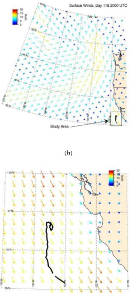
values (red line in Fig. 1a) reproduce the measured U10 values fairly well. Figure 3a

10

and b shows snapshots of COAMPS simulations of the large scale pattern of near-surface winds on YD 118 20:00 UTC overlaid on the drift track of FLIP. Evident in Fig. 3a is a large synoptic system that influenced the area on this day. A close look at the experimental site on YD 118 (Fig. 3b) shows strong wind speed (>12 m s−1) almost aligned with the coast line, as expected from the April climatology for this area (Wyllie, 15

1966; Chelton, 1984).

The air temperature (Fig. 1b) changed most noticeably on YD 113, from less than 10◦C to above 12◦C. In the period of radiometric data collection the air temperature remained relatively stable with diurnal variations also within 2◦C, between 12◦C and

∼14◦C. The seawater temperature in the mixed layer (0–10 m below MWL) was nearly 20

constant and uniform at∼13◦C (red symbols in Fig. 1b). The air–seawater temperature difference was within ±1◦C, primarily caused by diurnal variations. Relative humidity (Fig. 1c) was above 90 % initially, then dropped to around 70 % on YD 117. From YD 119 to YD 121, RH increased gradually back to∼90 %. In combination, these observa-tions suggest the existence of well-mixed boundary layers above and below the air–sea 25

interface with weak vertical heat flux, thus the atmospheric stability conditions can be characterized as near-neutral.

(19)

ACPD

14, 15363–15417, 2014

Title Page

Tables Figures

◭ ◮

Back Close

Full Screen / Esc

Discussion

P

a

per

|

Discus

sion

P

a

per

|

Discussion

P

a

per

|

Discussion

P

a

per

|

the FLIP location. Wind speed values were obtained from the COAMPS re-analysis output at 1 h intervals along the back trajectories out to 120 h earlier from the corre-sponding moment of data collection on FLIP. Back trajectories were calculated using the 3-dimensional velocity field from the re-analysis data from COAMPS, but with the vertical motion restricted to levels of constant potential temperatures (isentropic sur-5

faces).

Figure 4 shows back trajectories of air masses passing though the FLIP location daily at 20:00 UTC. The beginning of each trajectory is shown with the YD of arrival at the FLIP location. Wind speed history corresponding to each back trajectory is shown on the lower panel. These back trajectories show that the air mass at FLIP between 10

YDs 117 and 121 is clean marine air that has been propagating above the Northern Pacific for at least 5 days. This verifies that for the given time frame the aerosol com-position was predominantly of marine origin, and that the marine boundary layer had su_fficient time to get saturated with the sea spray aerosols. The back trajectory of YD 116 comes from the opposite direction, thus likely advecting continental air masses. 15

The full trajectory is not shown in Fig. 4 because it quickly exits the analysis domain.

4.2 Brightness temperature data

Brightness temperatures,T_B, from the 10.7 GHz radiometer are used in this study; data from the 37 GHz radiometer were found unusable due to a bias, which was not able to be replicated, most likely caused by an obstruction in its field of view.

20

Radiometric data were stored over discrete intervals of approximately 20 min during YDs 117–120. Less data was stored under conditions of low winds (e.g., two 20 min intervals per day) and more in high wind conditions with 5 to 23 20 min intervals per day. Total of 60 20 min intervals (i.e., 20 h) of data were recorded.

During each 20 min interval, the data were collected continuously at a sampling rate 25

(20)

ACPD

14, 15363–15417, 2014

Title Page

Tables Figures

◭ ◮

Back Close

Full Screen / Esc

Discussion

P

a

per

|

Discus

sion

P

a

per

|

Discussion

P

a

per

|

Discussion

P

a

per

|

allT_B samples within one 20 min interval were averaged to provide a single data point. Linear interpolation between the 20 min averaged values was used when necessary.

The resulting time series of brightness temperature at horizontal and vertical polar-izationsT_BHandT_BV, are shown in Fig. 1d. Both polarizations show a steady increase with increasing wind speed (Fig. 1d and a) over a range of∼10 K forT_BH(dashed blue 5

line) and a range of ∼5 K for T_BV (red solid line). The 10.7 GHz brightness tempera-ture variations are dominated by variation in the emissivity of the sea surface within the antenna footprint; the reflected downwelling brightness temperature arising from the atmosphere and cosmic background is a secondary factor. Figure 4 shows that these radiometric data were collected during days when clean marine air masses were 10

passing FLIP.

Various polarization di_fferences, polarization ratios, and variances were calculated and tested, and the key relationship in this study was found to rely on the di_fference in behavior between the vertically- and horizontally-polarized brightness temperatures. More specifically, the variables we found most useful in the analysis of data acquired 15

during BREWEX are defined as follows:

δTBP=TBP−TB0P=δTBrP+δTBfP, (9)

∆T_B=δT_BH−δT_BV, (10)

where δT_BP is the measured brightness temperature minus the modeled brightness 20

temperature of a flat surfaceT_B0Pin otherwise similar conditions (Eqs. 7 and 8b), cal-culated using the Meissner and Wentz (2004) model. Input parameters used in this calculation were the radiometer frequencyf =10.7 GHz, incidence angleθ=45◦, wa-ter temperatureT_s=13◦C, and salinityS=32.6 ‰, resulting in flat surface brightness temperature valuesT_B0H=81.8 K andT_B0V=140.2 K. The parameterδT_BP on the left 25

hand side of Eq. (9) is an attempt to minimize the dependence on these variables (i.e.,

(21)

ACPD

14, 15363–15417, 2014

Title Page

Tables Figures

◭ ◮

Back Close

Full Screen / Esc

Discussion

P

a

per

|

Discus

sion

P

a

per

|

Discussion

P

a

per

|

Discussion

P

a

per

|

valuesδTBrP+δTBfPin Eq. (8b). The parameter∆TBintroduced in Eq. (10) is the diff

er-ence between horizontal and vertical polarization ofδT_BPparameters. This parameter approximately removes foam contribution for low to moderate wind speeds, thus more accurately represents the roughness contribution alone (further discussed in Sect. 6.1).

4.3 Sea spray aerosol data

5

Aerosol data were collected from late YD 115 to YD 121. The PMS particle counter measures size-resolved aerosol concentrations, N(r), in the range from 0.25 µm to 23.5 µm by alternating every 4 s between four sub-ranges: 1.0 µm< r <23.5 µm, 1.0 µm< r <16.0 µm, 0.5 µm< r <8.0 µm, and 0.25 µm< r <4.0 µm. Particle counts in each sub-range are binned into 15 equally spaced bins according to radii. These out-10

puts were used to produce 20 min moving averages for each bin. Total aerosol concen-trations,N, are obtained by integrating over all radii. Figure 1e illustrates the resulting time series of raw droplet concentrations measured during BREWEX.

The most striking features in this time series are multiple concentration peaks during YD 116 and early 117, which are too high in magnitude to be correlated with the low 15

to moderate winds observed for the same period (Fig. 1a and e). Meanwhile, mea-surements ofN collected during higher winds after YD 117 appear to follow the wind speed intensity. A combination of these observations with the airflow direction reversal mentioned earlier (Fig. 4 and Sect. 4.1) suggests that the air masses passing through FLIP’s location on YDs 116 and early 117 might be contaminated by land and/or surf 20

zone aerosol sources. This would interfere with the requirement of the dry deposition method for steady production flux over a period of hours and even days. In addition, considering that the goal of this study is to investigate the relationship between the SSA production flux and surface brightness temperature, it is necessary that all data be associated with clean air masses so that the e_ffects of the local forcing (controlling) 25

(22)

ACPD

14, 15363–15417, 2014

Title Page

Tables Figures

◭ ◮

Back Close

Full Screen / Esc

Discussion

P

a

per

|

Discus

sion

P

a

per

|

Discussion

P

a

per

|

Discussion

P

a

per

|

analysis, from YD 117 to the end of the data collection, N steadily increased from

∼7×104to 2×105m−3as wind speed increased.

To remove the dependence of measured particle radius on ambient relative humidity, time dependent RH measurements were used to convert the mean droplet radius of each bin to the corresponding dry radius, r_dry, i.e., the radius of corresponding salt 5

particle without water (for details on this conversion see Gerber, 1985 and Andreas, 2002). Mean radius within each bin was calculated on a logarithmic scale.

To obtain the surface flux using the dry deposition method, all measurements of droplet concentrations,N(r), were converted to 10 m height reference using Eq. (3). The gravitational settling velocity was estimated with Eq. (2) using original non-dry 10

radius, and the wind friction velocity was calculated by logarithmically extrapolating measuredU₁₀ to the surface (Large and Pond, 1981). The sea spray surface flux at 10 m height, F(r_dry), was then calculated using Eq. (1). Results of these calculations were binned by equally-spaced logarithmic increments of dry radius and presented as flux per infinitesimal range of radii, dF(r)/d ln(r). Hereafterrrefers tor_dryand “ln” refers 15

to the natural logarithm.

Another output of the dry deposition method is the total surface flux integrated over all radii within the PMS measurement range, F_PMS. The subscript of F_PMS points out that this quantity is dependent on the radii cutoff range specific to the PMS instru-ment. Nonetheless, the total flux F_PMS, as opposed to the size-resolved production 20

flux dF(r)/d ln(r), is useful to study the sensitivity of the SSA surface flux to radiomet-ric brightness temperature,T_B. Within the data subset where simultaneous brightness temperature and SSA flux data are available, use of the total surface flux in this analy-sis helps to compensate for the reduction in the aerosol data sample size due to limited simultaneous radiometer uptime.

25

(23)

ACPD

14, 15363–15417, 2014

Title Page

Tables Figures

◭ ◮

Back Close

Full Screen / Esc

Discussion

P

a

per

|

Discus

sion

P

a

per

|

Discussion

P

a

per

|

Discussion

P

a

per

|

all data collected was used. Within this segment, wind speed held relatively steady atU₁₀≈11 m s−1. Concentration profiles were constructed based on data collected at three heights of 7.3 m, 6.0 m, and 4.9 m. Three consecutive profiles were measured within this time frame with sampling times at each level ranging from 30 min to 1 h. Samples at each height were averaged to form one vertical profile for the entire 7 h 5

segment. Additionally, only five radius bins (ranging from ∼1 µm to ∼3.5 µm) were found to contain a sufficient number of samples suitable for profile fitting. Resulting

N(z, r) profiles (Fig. 5) were fitted with best matching logarithmic curves to obtain

N_∗(r) in Eq. (4). Consequently, Eq. (5) was used to calculate surface flux, which was then normalized by ln(r) to match the format and dimensions of the dry deposition 10

method output. Note that the vertical deposition method provided only a few points at one wind speed. Therefore these points serve for reference and verification purposes, but unlike the output of the dry deposition method, are not su_fficient for full quantitative parameterization.

5 Results

15

The main objective of this study is to investigate the relationship between aerosol pro-duction flux and microwave brightness temperature of the sea surface. In this section, we present the analysis of the collected aerosol and radiometric data (Fig. 1) in pursuit of this goal.

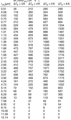
Figure 6 shows size-resolved sea spray source function dF(r)/d ln(r) (black circles) 20

in terms ofr_dryat four wind speeds obtained with the dry deposition method (Sect. 2.1.1 and 4.3). Surface fluxes obtained with the vertical gradient method from the available data (see Sect. 4.3) are also shown in Fig. 6 (black asterisks). SSA fluxes obtained with the SSSFs of Monahan et al. (1986) (blue solid lines) and Smith et al. (1993) (red dashed lines) for the same wind speeds as for the dry deposition method provide 25

(24)

ACPD

14, 15363–15417, 2014

Title Page

Tables Figures

◭ ◮

Back Close

Full Screen / Esc

Discussion

P

a

per

|

Discus

sion

P

a

per

|

Discussion

P

a

per

|

Discussion

P

a

per

|

The results of the vertical gradient method are approximately an order of magnitude higher than the results from the dry deposition method and those obtained with the pa-rameterization of Smith et al. (1993). This difference is discussed further in Sect. 6.2. The dry deposition method results compare fairly well with Smith et al. parameteriza-tion, which are based on a similar method. The comparison with the parameterization 5

based on the whitecap method (Monahan et al., 1983, 1986) shows agreement for larger droplets (r_dry>∼2 µm) and differences for smaller droplets with the parameteri-zation predicting much higher fluxes.

Figure 7 evaluates the sensitivity of the total SSA surface flux F_PMS (Sect. 4.3) to various input parameters, such that the vertical axis values remain constant across 10

all panels, but the horizontal axis changes depending on the chosen input parameter. In all four panels, individual data points (red dots) were obtained from the time series with 4 s sampling rate (Sect. 4.3) by first smoothing the time series by a 20 min moving average and then rarefying them (for presentation clarity) by averaging over every 20 consecutive aerosol data points. Trends (solid black curves) are obtained by linearly 15

connecting bin averages, where six equally-spaced bins are defined across the range of each input parameter. A 95 % confidence interval is shown for each bin-averaged point, calculated as 2σN_s−1/2, where σ is the standard deviation of the points in the bin andN_s is the number of samples in the bin. Figure 7a shows the wind speed de-pendenceF_PMS(U₁₀). This dependence is widely used to parameterize the surface flux, 20

but is known to have wide scatter, which is confirmed in the present figure. It is clear that the bin-averagedF_PMS(U₁₀) relationship alone is unable to completely capture the observed variability of the surface flux. In a quest for a better correlation between SSA surface flux and a local sea state parameter, we investigated relationships between

F_PMSandδT_BH,δT_BV, and∆T_B (see Sect. 4.2), shown in Fig. 7b–d. 25

(25)

ACPD

14, 15363–15417, 2014

Title Page

Tables Figures

◭ ◮

Back Close

Full Screen / Esc

Discussion

P

a

per

|

Discus

sion

P

a

per

|

Discussion

P

a

per

|

Discussion

P

a

per

|

dots in Fig. 7) are grouped closer together around their respective bin averages in

F_PMS(_∆T_B) than inF_PMS(U₁₀), resulting in tighter 95 % confidence intervals. The trend of the relationshipF_PMS(∆T_B) is more consistent and monotonic than that ofF_PMS(U₁₀) dependence (thick solid lines in Fig. 7a and d). Finally the sensitivity ofFPMS to these

di_fferent values may be compared by calculating the range of variation (F_max−F_min) in 5

the bin-averaged values over the full dynamic range for each parameter observed dur-ing the experiment. The resultdur-ing quantification demonstrates a significant advantage for_∆T_B:

(F_max−F_min)|_U₁₀=1771 [s−1m−2], (F_max−F_min)|δT_BV =1087 [s−1m−2],

(Fmax−Fmin)|δT_BH =1883 [s−1m−2],

(F_max−F_min)|_∆T_B=2706 [s−1m−2].

(11)

10

In other words, SSA surface flux was found to be the least sensitive toδT_BV, slightly more sensitive toδT_BH than to U₁₀, and by far the most sensitive to∆T_B, specifically 1.53 times more so thanU10 over the observed range of conditions.

For these reasons, brightness temperature polarization di_fference _∆T_B emerges as a sensitive and robust input parameter for estimating SSA surface flux, superior to the 15

wind speedU10or any other parameter tested here. This result is the key finding of this

study. The central practical question then is the feasibility of replacingU₁₀ with_∆T_Bso that the SSA surface flux is parameterized as dF(r,∆T_B)/d ln(r). Figure 8 and Table 1 demonstrate the utility of parameterizing SSA production flux in terms of brightness temperature polarization di_fference, as opposed to the conventional parameterizations 20

(26)

ACPD

14, 15363–15417, 2014

Title Page

Tables Figures

◭ ◮

Back Close

Full Screen / Esc

Discussion

P

a

per

|

Discus

sion

P

a

per

|

Discussion

P

a

per

|

Discussion

P

a

per

|

6 Discussion

The discussion in this section aims to understand the physical meaning of_∆T_B parame-ter in relation to aerosol production, make our case for using brightness temperature as an input variable for SSA surface flux parameterization, and lay initial groundwork for potential satellite remote sensing applications. Using the H12 model, we explore and 5

interpret the physical meaning of parameter∆T_Band propose an explanation for its rel-evance to the SSA surface flux (Sect. 6.1). We use the background information (Sect. 2) and our results (Sect. 5) to discuss existing uncertainties that ultimately motivate us to seek new alternative parameterizations (Sect. 6.2). We propose an empirical approach based on∆TB, which reduces some of these uncertainties (Sect. 6.3). A discussion of

10

the applicability of the proposed empirical approach for direct satellite remote sensing of SSA production flux follows (Sect. 6.4).

6.1 Physical interpretation of∆TBparameter

The H12 model (Sect. 2.2.4) can be used to interpret the parameters derived from the brightness temperature. Of specific interest are the wind-induced parametersδT_BH

15

and δT_BV, which contain contributions from both roughness and foam on the water surface, i.e.,δTBP=TBrP+TBfP(Eqs. 8b and 9). These are shown in Fig. 9a as functions

of wind speedU₁₀. The model calculates the contributions of surface roughness and foam separately. The modeled contribution of the foam term is also shown in Fig. 9a. The difference,δTBP−TBfP=TBrPcan be considered the contribution arising only from

20

surface roughness (not plotted to avoid cluttering).

The curves in Fig. 9a have a number of features significant for further discussion. First, comparison of δTBH and δTBV (solid and dash-dotted curves) exhibits the

ex-pected behavior that radiometric data atH polarization are more sensitive to sea state changes than those atV polarization, a result consistent with that seen in Fig. 7c and b 25