Solu¸c˜
ao Exata de Problemas de Escalonamento Determin´ısticos
por Meio de Verifica¸c˜
ao Exata de Modelos
Tese apresentada ao Curso de P´os-Gradua¸c˜ao em Ciˆencia da Computa¸c˜ao da Universidade Federal de Minas Gerais, como requisito par-cial para obten¸c˜ao do grau de Doutor em Ciˆencia da Computa¸c˜ao.
Belo Horizonte, Minas Gerais, Brasil
Universidade Federal de Minas Gerais - UFMG
This thesis was presented and approved at August, 30, 2002.
Prof. S´ergio Vale Aguiar Campos (Advisor)
Prof. Carlos Roberto Venˆancio de Carvalho
Prof. Henrique Pacca Loureiro Luna
Prof. Geraldo Robson Mateus
Prof. Edjard de Souza Mota
Uma se¸c˜ao de agradecimentos, em geral, simboliza o t´ermino de um trabalho. Confesso que, em alguns momentos, temi n˜ao chegar a esta se¸c˜ao. Contudo, v´arios fatores con-tribu´ıram para que eu lograsse ˆexito nesta empresa. Deus acima de tudo foi minha fonte de f´e: Ele n˜ao d´a a seus filhos um fardo que estes n˜ao possam carregar. Assim, acreditei e n˜ao me desviei do caminho.
Ao longo do caminho, deparei-me com v´arias pessoas. Algumas eu j´a conhecia outras n˜ao. Todas elas, direta ou indiretamente, me auxiliaram no doutorado. Quero expressar aqui a minha gratid˜ao a todas elas nominando-as uma a uma, tanto quanto me ´e poss´ıvel lembrar o nome de tantas pessoas (jur´ıdicas e f´ısicas).
O governo brasileiro atrav´es da CAPES apoiou-me finaneiramente ao longo do doutorado. A Universidade Federal de Uberlˆandia (UFU) e a Faculdade de Computa¸c˜ao (FACOM) ofereceram-me todas as condi¸c˜oes para que o meu doutoramento fosse realizado. A Universidade Federal de Minas Gerais (UFMG) e o Departamento de Ciˆencia da Com-puta¸c˜ao (DCC) tornaram dispon´ıvel os recursos necess´arios `a realiza¸c˜ao de meu trabalho.
Encontrei excelentes professores ao longo do doutorado. Alguns deles ser˜ao sempre referˆencias em minha vida profissional e pessoal: Berthier Ribeiro, Carlos Venˆancio, Clau-dionor Coelho, Edjard Mota, Edmundo Silva, Frederico Campos, Henrique Pacca, Newton Vieira, Robson Mateus, S´ergio Campos.
Andr´ea Iabrudi, Adriano C´esar, Camillo Jorge, Carlos Frederico, Denilson Barbosa, Gilberto Miranda, Gurvan Huiban, Hervaldo Sampaio, Hugo Barros, Ilm´erio da Silva, Jones Albuquerque, Jos´e Pio, Karla Borges, Linnyer Beatrys, Manoel Palhares, Marco Cristo, Maria de Lourdes, Mark Allan, Paulo Rodrigues, P´avel Calado, Ricardo Poley, Silvio Jamil partilharam comigo momentos inesquec´ıveis de cunho acadˆemico e/ou pessoal.
Bar-Alexandre Dias, Antˆonia Rocha, Belkiz Costa, Em´ılia Soares, Geraldo Oliveira, Gilberto Luiz Costa, Gustavo Oliveira, Helv´ecio Lopes, Maristela Soares, Luciana Costa, Renata Viana, T´ulia Andrade, por meio de seus respectivos trabalhos, tornaram minha vida muito mais confort´avel e agrad´avel no DCC.
Algumas pessoas tiveram uma rela¸c˜ao muita pr´oxima com o trabalho de tese. Jo˜ao Paulo Kitajima foi quem me incentivou a iniciar o doutorado, foi meu primeiro orientador e foi quem me propiciou minhas primeiras viagens ao exterior. S´ergio Campos, meu orien-tador, inspirou-me motiva¸c˜ao e confian¸ca. Suas interven¸c˜oes sempre corretas ajudaram-me a encontrar o rumo da tese e manter-me focado no mesmo. S´ergio possui um estilo de es-crita direto e fluido que determinou meu estilo de eses-crita atual. Hervaldo Sampaio, m´edico e contemporˆaneo de doutoramento no DCC, dispendeu parte de seu tempo para pesquisar artigos m´edicos sobre Refluxo V´esico-Ureteral, uma anomalia que minha filha Daniela teve no in´ıcio de sua infˆancia. Gurvan Huiban, parceiro de rep´ublica e de doutorado, ajudou-me com experimentos com a ferramenta CPLEX. Hugo Barros ajudou-me com a programa¸c˜ao de uma ferramenta para gera¸c˜ao autom´atica de modelos SMV. Adriana Mariano ajudou-me a manter-me focado no doutorado.
Finalmente, gostaria de dizer algumas palavras sobre pessoas muito especiais para mim. Eu tenho pais maravilhosos, que s˜ao minha fonte de inspira¸c˜ao. Ao longo de todo o tempo de doutorado, sempre estiveram presentes em minha mente e em meu cora¸c˜ao. Eu tenho um irm˜ao, que acima de tudo ´e meu melhor amigo. Eu tenho quatro filhos que s˜ao a raz˜ao de minha vida, a raz˜ao do meu respirar. Eu tenho um amigo, Lu´ıs Carlos R´ıspoli, que desencarnou num acidente automobil´ıstico. A todos eles pe¸co desculpas pela minha ausˆencia durante esses ´ultimos anos . . . E no final de tudo, eu a encontrei. Ela passou em minha vida como a brisa da manh˜a, suave e fugaz, mas foi suficiente para se tornar inesquec´ıvel.
Problemas de Scheduling est˜ao relacionados com o sequenciamento de um conjunto de atividades a serem executadas por um conjunto de recursos ao longo de um determinado pe´ıodo de tempo. Este tipo de problema possui diferentes configura¸c˜oes. Neste trabalho focamos uma classe de problema conhecida como problemas deterministico-est´aticos. N´os apresentamos Verifica¸c˜ao Simb´olica de Modelos (VSM) como uma nova abordagem de solu¸c˜ao para esta classe de problemas.
VSM ´e uma t´ecnica de verifica¸c˜ao formal que tem alcan¸cado ˆexito na verifica¸c˜ao de diferentes sistemas complexos. N´os temos utilizado VSM para dar solu¸c˜ao exata a prob-lemas determin´ıstico-est´aticos do tipo job-shop e flow-shop. Ao longo deste trabalho, n´os apresentamos a modelagem e os resultados que obtivemos na solu¸c˜ao destes problemas. Finalmente, n´os apontamos tamb´em dire¸c˜oes futuras para este trabalho.
Scheduling relates to ordering a set of activities to be performed by a set of resources over a period of time. Scheduling ranges over a very large variety of problems, however we are concerned with deterministic static scheduling problems. In this thesis, we present Symbolic Model Checking (SMC) as a new approach to solve this class of problem.
SMC is a finite state formal verification technique that has been successfully used to verify many complex systems. We have been using SMC to give exact solution to deterministic static scheduling problems, such as job-shop and flow-shop problems. We present the modeling and the results we have obtained solving some instances of these problems, and finally, we point out future directions to this work.
1 Introduction 1
1.1 Motivation . . . 1
1.2 Traditional Approaches . . . 2
1.3 Symbolic Model Checking . . . 3
1.4 The Proposed Approach and Results . . . 3
1.5 Contributions . . . 6
1.6 Organization of the Thesis . . . 6
2 Symbolic Model Checking - SMC 7 2.1 Model Checking - MC . . . 8
2.1.1 Kripke Structure . . . 9
2.1.2 CTL - Computation Tree Logic . . . 12
2.1.3 A Microwave Example . . . 16
2.1.4 CTL Model Checking . . . 17
2.2 Symbolic Model Checking - SMC . . . 18
2.2.1 Ordered Binary Decision Diagrams - OBDDs . . . 19
2.2.2 The Model . . . 19
2.2.4 SMV - An OBDD Symbolic Model Checking Tool . . . 22
2.2.5 Verus - A Symbolic Model Checking Tool for Real Time Systems . . 25
3 Symbolic Model Checking over a Video on Demand System 28 3.1 The ALMADEM-VOD Server . . . 29
3.2 Modeling the ALMADEM-VOD Server in Verus . . . 34
3.3 Results . . . 36
3.4 Conclusion . . . 39
4 Scheduling 41 4.1 Basic Concepts . . . 42
4.1.1 Workshops . . . 44
4.2 Traditional Approaches to Job-Shop Problem . . . 46
4.3 Conclusion . . . 48
5 Symbolic Model Checking Applied to Deterministic Scheduling Prob-lems 50 5.1 Modeling JSP into OBDD Domain . . . 50
5.2 Modeling Job-Shop Problems into SMV . . . 53
5.3 Computing Makespan . . . 58
5.4 Conclusion . . . 61
6 New Model Checking Algorithms 63 6.1 MINCOND Algorithm . . . 64
6.2.1 MINCOND-P application . . . 70
6.3 MINCOUNT-P Algorithm . . . 71
6.3.1 MINCOUNT-P application . . . 73
6.4 Conclusion . . . 74
7 Integration between Production and Operational Planning 75 7.1 Integrating Information between Tactical and Operational Levels . . . 76
7.2 Multi-Period Scheduling Problem . . . 77
7.3 Modeling Multi-Period Job-Shop into SMV . . . 80
7.4 Conclusion . . . 85
8 Conclusion and Future Works 86 8.1 Future Works . . . 88
A Instances of JSP and FSP 90
B Mixed Integer and Linear Programming Model for JSP 94
5.1 Description of an hypothetical manufacturing industry problem. It presents the demanded time and execution ordering to produce automobile’s front panels. . . 53
5.2 Consumption of OBDD nodes, time and memory by SMV when executing some flow-shop and job-shop problems. The column ”time” is in seconds, except in the 6×6 job-shop cell, that is in minutes. . . 59
5.3 Time comparison (in seconds) between SMV and CPLEX in computing the makespan of some JSPs and FSPs. . . 60
2.1 A program example and its correspondent Kripke structure. . . 11
2.2 Linear and branching-time structure of time of temporal logics. . . 12
2.3 A Kripke structure and a relating computation tree. Kripke state labeled to ”a b” was taken as root and the Kripke structure was unwinded from this state. The unwinding process generated an infinite tree over which CTL is applied to. . . 13
2.4 Basic CTL operators over a computation tree. The black states represent the states in which proposition g holds. The ”s” designates the state taken as root. This figure presents the configuration of computation trees so that the respective CTL operator can yields to true. . . 15
2.5 A Kripke structure representing a microwave. . . 16
2.6 Binary decision tree (on top) and a correspondent OBDD (below) for the boolean formula (a∧b)∨(c∧d). The dashed arc is taken when var(v) = 0. The solid arc is taken when var(v) = 1. . . 20
2.7 Example of a transition and its symbolic representation. . . 21
2.8 The MIN algorithm determines the minimum path between states∈S and state f ∈F, in a breadth-first search way. . . 22
2.9 A SMV model for the microwave example presented in Section 2.1.3. . . . 23
2.10 A Verus program that models a non-deterministic event and its respective alarm. . . 26
3.1 Overall architecture for a video service. . . 28
3.3 Service cycle with a duration of T seconds. ts accounts both for seek and rotational delay times. . . 31
3.4 Service cycle occupation in the ALMADEM-VOD server for periods varying from 1s to 9s. The number of clients in the system is 20. . . 33
3.5 An illustration of the ALMADEM-VOD server specification in Verus. . . . 35
3.6 Variation of the service time occupation by clients for the server and for Verus (T = 4s). . . 36
3.7 Service time for the ALMADEM-VOD server and for the revised Verus model (T = 4s). . . 37
3.8 Synchronization of disk and network threads through a pair of signal and wait primitives. . . 39
3.9 Service time for the new versions of the server and of the Verus model (T = 4s). 40
4.1 A taxonomy for scheduling problems. The shaded rectangle represents the class of deterministic static scheduling problems that is the focus of this thesis. 43
4.2 The structure of flow-shop. . . 44
4.3 The structure of an open-shop. . . 45
4.4 Disjunctive graph representing a job-shop 3×3 (3 jobs in 3 machines) . . . 47
5.1 An OBDD representing the ordering for the conclusion of task 7. The boolean variablescxandcy represent hypothetical machinesxandy, respec-tively. In this illustration the machines are represented by a 3-bit counters. Machine x is the one that runs task 7, and machine y runs task 6. Task 7 can be run only if task 6, technological precedence of 7, is finished. Task 6 is finished when all boolean variables representing machine y is zero. Task 7 is finished when can reach the terminal node 1, and there is only one path to it. . . 52
5.4 Excerpt of our SMV program relating to a machine that chooses one task among two of them to run. . . 57
6.1 The MINCOND algorithm and an illustration of its behavior. . . 64
6.2 Gantt chart for the 3×3 job-shop relating an hypothetical manufacturing industry of automobile front panels described in Table 5.1. This illustration presents a sequence of tasks that results in a minimum makespan. . . 66
6.3 Gantt chart for the 3×3 job-shop relating an hypothetical manufacturing industry of automobile front panels. This illustration presents a sequence of tasks in which Panel A finishes as soon as possible but minimizes the late of the other tasks. . . 67
6.4 The MINCOND-P algorithm and an illustration of its behavior. This algo-rithm searches for paths between states I and F, in which all states along the path satisfy condition C. If MINCOND-P finds such paths, it returns the size of the shortest one. Otherwise MINCOND-P returns infinity. The illustration presents a case in which F is reached in 4 steps. . . 69
6.5 Gantt chart for the 3×3 job-shop problem example, considering that ma-chines 1 and 3 can not run in parallel anymore. . . 71
6.6 MINCOUNT-P algorithm returns a path between state I and F, such that in this path m states satisfies C. m is the least number of states satisfy-ing C over all paths leading from I to F. If there is no path between I and F, MINCOUNT-P returns the special value NOPATH. If m= 0, then MINCOUNT-P returns∞ (infinity). The illustration shows the behavior of the algorithm. It walks backward reaching states over paths between I and F. In this illustration, we can see that I is reached in 5 steps. . . 72
7.1 A 3×3 JSP represented as disjunctive graph (on top) and an optimal se-quence for the corresponding makespan represented by a Gantt chart (in the bottom). . . 78
7.2 Model for exchange of information between tactical and operational level. . 79
as NP and t y.pwherey={1,3,4,6}. Variable t 1.p, for example, indicates in
which period t 1 has been done. . . 81
7.5 Excerpt of our SMV model for a task of a multi-period JSP. . . 83
7.6 Excerpt of our SMV model for a machine that runs two tasks in an multi-period JSP. . . 84
7.7 Makespan for a JSP 3×3 of 3 periods. . . 85
B.1 MILP model for JSP 3×2. . . 95
Introduction
1.1
Motivation
Scheduling relates to ordering a set of activities to be performed by a set of resources over a period of time. Scheduling problems arise when the necessary resources for perform-ing the activities are scarce. Due to this scarcity it becomes essential to determine the best order of execution for all activities. Determining the best order implies in scanning a space that have a finite or countably infinite number of possible solutions. This class of problem is known to be NP-Hard. Therefore, depending on the size of the instance problem, it is necessary the use of appropriate tools to get a feasible solution.
Scheduling problems range over a great variety of domains. We can find scheduling problems in areas, such as manufacturing, publishing, transport, health, computing, etc. For this reason, scheduling problems have different classes of problems. We are concerned with a class in which all parameters about resources and activities are stated in advance. This class of problems is known as deterministic static scheduling problems. For now on, we refer to activities as jobs and resources as machines.
The main objective of this work is to explore the application of formal methods to the solution of scheduling problems. Specifically we are applying a formal method based in a temporal logic model checking technique. This technique is known as Symbolic Model Checking (SMC). SMC models a problem as finite state transition graph. Efficient algo-rithms traverses the state space searching for model properties. The properties are specified using temporal operators or quantitative algorithms.
this class of problems. SMC is a general problem solver in opposite to certain traditional tools. Being so, SMC provides great flexibility to solve a wide range of scheduling. Be-sides, the efficiency of its algorithms and its internal representation allows the modeling of complex instance problems.
1.2
Traditional Approaches
Researchers have studied many different scheduling problems. There are problems involving one machine, several machines, related and unrelated machines. Besides, there are also different job characteristics and optimality criteria to consider. In common with all of them is that the great majority of this problems are NP-Hard. This implies that it seems unlikely that there is a polynomial time algorithm relating the size of the input problem that gives an exact solution to them. Therefore there are different approaches to cope with them.
Some approaches consist of relaxing the restrictions of the problem. The relaxation makes the problem simpler and consequently easier to solve. For example, the problem of non preemptive scheduling of independent jobs on two identical processors, and minimum makespan as optimization criterion is NP-hard; but if we relax this problem by allowing preemption it becomes an O(n) complexity time problem [12], where n is the number of jobs. In general, the relaxation is used to help in the design of approximation algorithms.
Among approximation algorithms, there are also different approaches to cope with scheduling problems. There areconstructive methodsin which one important representative is the shifting bottleneck heuristic [2, 8]. There are also iterative methods in which we can find thelocal search algorithms that comprisestabu search,simulated annealing [4, 9], and genetic algorithms [54]. All these algorithms are very efficient and in some cases are used to determine bounds to certain exact approaches.
modification and re-implementation.
1.3
Symbolic Model Checking
Symbolic Model Checking (SMC) [66] is an automatic formal technique proposed for verifying finite states concurrent systems. SMC models a system being verified as a state-transition graph. Properties about the model are specified in a temporal logic. The model checking process consists of exploring all states of the model to determine if the specified properties are satisfied. This verification always terminates and the truth value of the properties are presented. When any property is falsified, SMC is able to give a counter-example: a path in the model that demonstrates the property falsification. Counter-example is a trace of states that presents a possible computation in which the model does not satisfy the property. It is a very important tool for debugging systems. It generally provides very good insights about the erroneous behavior of the system being modeled.
SMC has been successful in verifying several large and complex systems such as the Futurebus+ protocol [30] and the PCI bus performance [18]. States and transition between states of the model are represented symbolically by boolean formulas and implemented by OBDDs [17]. The use of OBDD allows SMC to verify systems with as many as 1030
states (in some specific cases it was already reached 10120
states [31]).
1.4
The Proposed Approach and Results
Symbolic Model Checking (SMC) is a temporal formal method technique appropriate to finite states systems. Since solving scheduling problems consists of identifying a feasible solution over all possible solutions, SMC is very appropriate to this class of problem. The underlying model of SMC and its basic model checking algorithms can solve many class of scheduling problems, such job-shop problem (JSP). In this case, SMC is able to compute the minimum makespan, that corresponds to a sequence of jobs over machines such that this sequence imposes the least minimum time to accomplish all jobs. In SMC, computing the minimum makespan of a JSP, for example, reduces to the reachability problem between two states of the model.
adequate to some new circumstances. For example:
1. one needs to determine a new minimum makespan since a specific job must finish before all others. It is not the case of simply computing the new makespan not consid-ering this specific job. Again, SMC answers this question by evoking an appropriate quantitative algorithm combined with an appropriate temporal logic property.
2. one needs to determine a new makespan, since, for some reason, he/she needs now to serialize two specific machines. We will see that we can deal with this restriction only evoking a quantitative algorithm with an appropriate CTL property;
Our study about SMC has begun in the context of a Video on Demand (VOD) System. At first, we have applied SMC to determine the nominal capacity of a multimedia server [11, 21]. We have analyzed the ALMADEM-VOD server a component of a VOD system. We have determined the performance bounds to the server, and these bounds have pointed out to a discrepancy with the actual server. The discrepancy was analyzed and an error was found in the code of the server. After correcting this error, ALMADEM-VOD improved its performance (number of clients being served at the same time) in 40%.
After VOD work, we have started the study about scheduling which involved the ap-plication of SMC in solving some class of scheduling problems known as flow-shop and job-shop problems. We have modeled job-shop problems into SMC and computed the min-imum makespan of some non-trivial instances [63]. We have determined, for example, the minimum makespan of a job-shop 6×6 (six jobs in six machines), whose solution spaces is around (6!)6
possible sequences.
SMC can be seen as a finite state problem solver tool box. When the current symbolic algorithms are not well appropriate to deal with a specific problem, we can implement new algorithms and incorporate them into the tool box. It is important to mention that no modification is necessary to the original verification algorithms already installed. Indeed, in this work, we present three new algorithms that we have implemented to cope with scheduling problems: MINCOND, MINCOND-P, and MINCOUNT-P.
that along this minimum path the condition is satisfied at least once. That is the case of example 1 above.
MINCOND-P is slightly different from MINCOND. MINCOND-P returns the size of the shortest path (i.e. number of edges) betweensI andsF, such that conditionC holds in ALL states of the path that precedes sF. MINCOND-P starts fromsI searching for paths that lead tosF. However, only states that satisfy C are considered. This algorithm is very useful to deal with problems like ”what is the new makespan since machine 1 and machine 3 can not run in parallel anymore?” This is the case described in example 2 above.
MINCOUNT-P is an extension to the algorithm MINCOUNT [22]. Consider π1, π2, . . . , πpbeing all paths between statessIandsF. MINCOUNT searches for states that
satisfies a conditionC along the pathsπi, 1< i < pand returnsm =min(m1, m2, . . . , mp)
such that mi is the number of states satisfying C along the path πi. MINCOUNT-P ex-tends MINCOUNT by presenting the path relating to m. This algorithm is very useful when we are facing problems like the following. In many manufacturing industries, the jobs can be processed by anyone of the machines of the production line. If we want to determine a sequence for the jobs over the machines, such that the makespan is minimum and some specific machine is used as less as possible, then the MINCOUNT-P does this task.
Several examples have been applied to MINCOND and MINCOND-P. The results have confirmed the viability of the approach. SMC has correctly computed the minimum makespan of the problems, and SMC indeed has served as tool box.
1.5
Contributions
In this work we have proposed the application of SMC (a formal method technique) to give exact solution to scheduling problems. The model checking approach assures the correct answer to different questions that can occur in a plant, for example. These questions can appear in unexpected fashion and in general can be answered by SMC only by using appropriate algorithms and/or specifying a correspondent CTL formula.
The algorithms we have proposed enhance the capability of SMC as finite state general problem solver. It implements some features that are not obtained directly by original CTL formulations.
We also have presented new algorithms that enhance the verification power of SMC. Besides we have presented SMC models for job-shop, flow-shop and integration decision planning problems.
The SMC approach to scheduling problems also opens up new possibilities to two independent research groups: Combinatorial Optimization and Formal Methods. To the former, it offers a new view of how to solve this kind of problems. Since SMC makes available temporal logic feature, it can be used to determine if is possible to get some job finished before a given deadline, for example. To the latter group, it offers a great amount of research about how to deal with big state space.
1.6
Organization of the Thesis
Symbolic Model Checking - SMC
Formal Methods (FM) are mathematical based techniques and tools for specifying and verifying systems. Specification techniques are used to formalize the requisites and proper-ties of a system and its product usually can be converted in system documentation. Some examples of specification techniques/tools are Z [77], VDM [58], CSP [53]. Verification techniques and tools go one step beyond. They are able to help the system designer to find errors in the system. The system is modeled in a suitable language and properties about the system can be verified. Some examples are SMV [66], CV [39]. Other examples of specification and verification techniques/tools as well as real case applications of FM can be found in [81, 32].
Many verification techniques and tools in general are very known by Theorem Provers and Model Checkers. In both of them the verification process comprises three phases [66, 55]:
Modeling - description of characteristics and behaviors of the system in a given language;
Specification - description of the system’s properties that we want verify; and
Verification - execution of the verification process in order to determine if the properties hold for the model.
In the Model Checking (MC) approach, the system is modeled for an appropriate logic. The model (M) is finite and the specification is described as formula φ. The MC process consists of verifying whether M satisfies φ by scanning all reachable states of M from a state s of this model. This process can be represented mathematically by M, s|=φ.
The MC approach is more restrictive than TP approach in the following aspects: (1) it deals with finite systems; (2) it proves the satisfiability of φ with respect toM, not to all modelsM, such thatM |=φ. These aspects make TP a more general technique than MC approach. However, they also confer important features to MC that usually are not present in TP. In general, the MC verification process is fast and fully automatic. Besides, MC is able to present acounterexample, when φis falsified. Counterexample is a computation sequence in the model that proves that M |=/φ.
This chapter presents Symbolic Model Checking (SMC), a representative of MC ap-proach, that is the tool used in this thesis to exactly solve scheduling problems. Initially, we make a review about MC formalism concerning Kripke structure, the underlying model of MC, and Computation Tree Logic, a temporal logic that is used to reason about the modeling systems. We also present how a simple microwave is modeled by a Kripke structure and how CTL can reason about this model, concerning a microwave property. After that, we make a review about SMC focusing its symbolic model and OBDD, the data structure used to implement this model. We also present a basic SMC search algorithm used to find the minimum path between two states of the model. This algorithm is used in this thesis to solve some scheduling problems and has inspired some new algorithms presented in Chapter 6. Finally, we present two SMC tools that we have used along this thesis: SMV and Verus.
2.1
Model Checking - MC
MC is a technique originally proposed to deal with finite states systems 1
. The system being verified is represented by an appropriate model and the properties we want to verify are specified in a correspondent reasoning system. The MC process consists in scanning (all) states of the model to check if the model conforms the properties. Although MC approach can only deal with finite states systems, there are important systems that fall into this class, such as digital circuit design and communication protocols.
1
MC technique has some variants. Temporal logic model checking [29, 74] represent the system as finite state transition graph and a temporal logic [64] is used to specify properties about the system. Efficient algorithms search the state space to check if the model satisfies the properties. In automata approach, the system and the properties are represented as automata. Then, the system is compared to the properties to determine if they hold to the system. This comparison is accomplished by techniques such as language inclusion, refinement orderings, and observational equivalence [32]. Another approach is model checking by using integer linear programming (ILP) [33, 28]. In this approach, the system and the properties about the system are modeled as a linear inequality system. The equations relating to the the system properties are expressed in a such way that model the properties that the system should not have. The inequality system then is applied to an ILP method. If an integral solution is found then the system has the necessary conditions for the violation of the system properties.
The MC approach we will strengthen here is the temporal logic model checking. Finite states transition systems are modeled as Kripke structure and a temporal logic is used to specify properties.
2.1.1
Kripke Structure
Kripke structure [31] is a well known model for finite states transition systems. For-mally, let AP be a set of atomic proposition. A Kripke structure K over AP is a 4-tuple (S, S0, ρ, L), where S is a finite set of states, S0 is the set of initial states, ρ ⊆ S×S is a
transition relation (that is total - that is, all states have successors), andL:S →2AP is a function that labels each state with the set of propositions true in that state.
A state in a Kripke structure represents a snapshot of the system being modeled. The system is represented by a set of variables and each state represents the valuation of these variables in a specific moment. Considering D a finite set and V = {v1, v2, . . . , vn} the
variables of the system, the valuation for s ∈ S is the result of the function s : V → D, that associates a value inD for each variable in V.
The Kripke structure use formulas of propositional logic to represent states. Let D =
{F ALSE, T RUE}andV ={v1, v2, v3}, the valuation (v1 ←T RUE, v2 ←F ALSE, v3 ←
T RUE) can be expressed by the following formula of the propositional logic (v1 ∧ ¬v2 ∧v3).
The propositional logic is also used to represent the transition between states. To this extent another set of variables V′ is created, such that for each v ∈ V there is a corresponding variablev′ ∈V′. Variables in V are used to represent the current state and V′ to represent the next state. A valuation toV and V′ corresponds to setting an ordered pair of states, and can be expressed by formulas as before. For instance, consider that the current states are represented by the formula (v1 ∧ ¬v2 ∧ v3), if in the next state
v1 ←F ALSE, then the transition between the current to the next state can be expressed
by the formula (v1 ∧ ¬v2 ∧ v3 ∧ ¬v′1 ∧ ¬v′2 ∧ v′3). The set of transitions of a system
is referred to as transition relation, and if ρ represents a transition relation, then ρ(V, V′) denotes a formula that expresses it.
Finally, let us consider the set of atomic propositionsAP. Each atomic proposition has the form v =d, where v ∈ V and d ∈ D. An atomic proposition v = d is true in a state s, if s(v) =d. When v ranges over boolean domain{TRUE, FALSE}, we write v to mean s(v) =T RUE and ¬v to mean s(v) =F ALSE.
We now show how Kripke structure K = (S, S0, ρ, L) models a system from
proposi-tional formula SI and from the system R.
• S is the set of states consisting of all possible valuations for V;
• S0, initial states, is the the set ofs ∈S such that satisfies the formula SI;
• ρ⊆S×S is the transition relation. ρ(s, s′) holds ifRyields to true when eachv ∈V and eachv′ ∈V′ is assigned tos(v) ands(v′), respectively;
• L:S →2AP is the function that labels the states. L(s)⊆AP is the set of p∈AP, such thatp is true.
A computation in the system is represented by a path inK. A valid path from a state s is an infinite sequence of states π = s0s1s2 . . . , such that s0 = s and ρ(si, si+1) holds
∀i≥ 0. As an example, consider the program of Figure 2.1-a. According to this program V ={x, y},D={0,1}. The set of initial states is represented bySI(x, y)≡(x= 0)∧(y= 1) and the transition relation by ρ(x, y, x′, y′) ≡ (x′ = y)∧(y′ = y). The corresponding Kripke structure K = (S, S0, ρ, L) to these formulas is the following:
• S ={(0,0),(0,1),(1,0),(1,1)} • S0 ={(0,1)}
• L((0,0)) = {x = 0, y = 0}, L((0,1)) = {x = 0, y = 1}, L((1,0)) = {x = 1, y = 0}, L((1,1)) ={x= 1, y = 1}
The Figure 2.1-b illustrates K. The states are numbered only to ease the explanation about this figure. Observe that starting from S0 states 1 and 2 are not reachable.The
only valid computation in this system is that related to the path 0,3,3,3,3,3,. . .
example {
procedure
var
begin
while (true)
end
}
x := 0;
y := 1;
x = y;
(x = 0) ^ (y = 1)
(x = 0) ^ (y = 0) (x = 1) ^ (y = 0)
(x = 1) ^ (y = 1)
( x = 0 ^ y = 1 ) ^ ( x’ = 1 ^ y’ = y ) ( x = 0 ^ y = 0 ) ^
( x’ = 0 ^ y’ = y )
( x = 1 ^ y = 1 ) ^ ( x’ = 1 ^ y’ = y ) ( x = 1 ^ y = 0 ) ^ ( x’ = 0 ^ y’ = y )
0 2
3 1
Figure 2.1: A program example and its correspondent Kripke structure.
Definition 2.1 A state sn is reachable from a states0, if there is a path π =s0s1s2. . . sn
Linear temporal domain representaion
Branching−time domain representaion
Figure 2.2: Linear and branching-time structure of time of temporal logics. .
2.1.2
CTL - Computation Tree Logic
Temporal logic is a formalism very useful to describe sequences of transitions between states [66]. With temporal logic we are able to reason about the system in terms of occurrences of events. For example, given a model K the temporal logic offers reasoning power to determine if a certain event willeventually occur or if it always occurs.
There exists several types of temporal logic [72]. These logics vary according tempo-ral structure (linear or branching-time) and time characteristic (continuous or discrete). Linear temporal logicsreason about the time as a chain of time instances. Branching-time logics reason about the time as having many possible futures from a given instance of time. (See figure 2.22
.) Time is continuousif between two instances of time is always possible to find another one. Time is discrete if between two instances of time is not always possible to find another one.
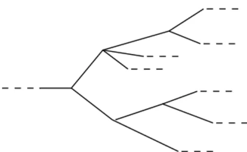
The logic of our study is a branching-time and discrete one known as Computation Tree Logic (CTL) [29]. Its name is due to the reasoning over trees of computation. The tree is (metaphorically) obtained unwinding the Kripke structure from a determined state (taken as root). Figure 2.3 presents an example.
CTL provides operators to be applied over the paths formed by the computation tree. When these operators are specified in a formula they must appear in a pair and in this order: path quantifier followed bytemporal operator. A path quantifier defines the scope of
2
c
Kripke Structure a b
b c
c c
c a b
b c
a b
Infinite Tree
Figure 2.3: A Kripke structure and a relating computation tree. Kripke state labeled to ”a b” was taken as root and the Kripke structure was unwinded from this state. The unwinding process generated an infinite tree over which CTL is applied to.
the paths over which a formulaf must hold. There are two path quantifiers: A, meaningall paths; andE, meaning somepath. A temporal operator defines the appropriate temporal behavior that is supposed to happen along a path relating a formula f. The temporal operators are the following:
• F(”in the future” or ”eventually”) - starting from the root,f holds in some state of the path;
• G(”globally” or ”always”) - starting from the root,f holds in all states of the path;
• R (”release”) - there is a state s in the path where formulas f and g hold and all preceding states froms does not satisfies f;
• U (”until”) - there is a state s in the path where a formula g is satisfied and all predecessor states ofs satisfiesf.
• X (”next time”) - starting from the root,f holds in the second state of the path.
A well formed CTL formula is defined as follows:
1. T RUE,F ALSE are CTL formulas;
2. If p∈AP, thenp is a CTL formula, such that AP is the set of atomic propositions; 3. If f and g are CTL formulas, then¬f,f∨g, f∧g, AFf, EFf, AGf, EGf, A[fRg],
Considering the Kripke model M = (S0, S, ρ, L), we denote that M satisfies a CTL
formula f from a state s∈S as
M, s|=f
Letf and g be CTL formulas, the satisfaction relation |= is defined inductively as follows [55]:
M, s|=T RUE and M, s|=F ALSE for all s∈S M, s|=p ⇔p∈L(s)
M, s|=¬f ⇔M, s6|=f
M, s|=f ∨g ⇔M, s|=f orM, s|=g M, s|=f ∧g ⇔M, s|=f and M, s|=g
M, s|=AF f ⇔for all paths from s, sk ∈S is reachable andsk |=f M, s|=EF f ⇔for some path from s, sk ∈S is reachable and sk |=f
M, s|=AGf ⇔for all paths π=s0s1s2. . . , si |=f, for all i≥0, ands0 =s
M, s|=EGf ⇔for some path π =s0s1s2. . . , si |=f, for alli≥0, and s0 =s
M, s|=AXf ⇔for all sx such thatρ(s, sk) is defined, sk |=f
M, s|=A[f Ug] ⇔for all paths π=s0s1s2. . . sk. . . , si |=f,0≤i < k and sk|=g
M, s|=E[f Ug] ⇔for some path π =s0s1s2. . . sk. . . , si |=f,0≤i < k and sk |=g
M, s|=A[f Rg] ⇔for all paths π=s0s1s2. . . sk. . . , si 6|=f,0≤i < k and sk|=g
M, s|=E[f Rg] ⇔for some path π =s0s1s2. . . sk. . . , si 6|=f,0≤i < k and sk |=g
Despite all combinations we can get with path quantifiers and temporal operators pre-sented above, we can express any CTL formula using∨, ¬, EX, EU, EG[31]:
• AFf =¬ EG ¬f
• AG f = ¬ EF ¬f
• AX f = ¬ EX ¬f
• A[f U g ] ≡ ¬ E[¬g U (¬f∧ ¬g)]∧¬ EG¬g
• A[f R g] ≡ ¬E[ ¬f U¬g]
• EF f = E[⊤U f]
Figure 2.4 presents the computation of the most frequently used CTL operators. Some typical examples of CTL formulas relating to concurrent reactive systems are presented below.
EF(started∧ ¬ready) - it is possible to get to a state wherestartedholds but ready does not hold.
AG(req → AFack) - it is always the case that if the signal req is high, then eventually ack will also be high.
A[greenLight U armMoves ] - it is always the case that the robot’s arm moves after the green light is on;
E[greenLight R armMoves ] - it does exist a situation in which the robot’s arm moves before green light is on;
M, s |= EG g M, s |= AG g M, s |= AF g M, s |= EF g
s s
s s
g
g
g g
g
g
g g g
g g g
g g
setup door−open ¬cooking setup ¬door−open cooking setup ¬door−open ¬cooking ¬setup ¬door−open ¬cooking ¬setup door−open ¬cooking setup cook pause open open close cancel
timeout / cancel
cancel
setup
open
close
Figure 2.5: A Kripke structure representing a microwave.
2.1.3
A Microwave Example
We present an example of verification using CTL logic. The example is about a simpli-fied microwave, inspired in a similar example given by Clarke, Grumberg, and Peled [31]. The possible operations in our microwave are the following: (a) we can open or close the door of the microwave; (b) we can set the time of cooking; (c) we can cook; (d) we can pause or cancel the cooking; (e) we can restart the cooking; and (f) the microwave turns itself off after the time of cooking is over - timeout. This microwave can be modeled by three boolean variables:
setup represents the parameters of the microwave set by user, such as time of cooking;
door-open indicates whether the door of the microwave is opened or not;
cooking indicates if the microwave is cooking the meal.
A very important (life) safety property concerns with cooking with door opened. We can verify this property with CTL logic by expressing
AG(cooking → ¬doorOpened)
We can simplify this formula in terms of equivalent ones:
AG(cooking → ¬door-open) ≡ ¬EF¬(cooking→ ¬door-open) ≡ ¬EF¬(¬cooking∨¬door-open) ≡ ¬EF(cooking∧door-open)
Therefore, we need to find out if there exists a state in the model such that the proposition
cooking∧door-openholds in any state. Since there is no state that satisfies this proposition, the model satisfies the property ¬EF(cooking ∧ door-open).
2.1.4
CTL Model Checking
CTL model checking consists of searching for states of Kripke model with label f, where f is a CTL formula. The set of states labeled to f are the ones that satisfies the formula. Formally, let f be a CTL formula and label(s) be the set of subformulas of f that are true ins∈S. The CTL model checking problem is related to determining the set S ={s | M, s|=f → f ∈label(s)}.
The model check process has two phases: translation and labelling. The translation phase consists of rewriting a CTL formula in terms of¬,∨, EX, EG, and EU. The labelling is a process of i steps, where i is the number of sub-formulas of f. In each ith step, the i−1 nested CTL operator (sub-formula) labels a state if the sub-formula is true in that state.
The labelling process observe the following rules:
• labels to p, ifp∈AP and p∈L(s);
• labels to ¬f1, if s is not labeled with f1
• labels to f1∨f2 ifs is labeled with f1 or with f2;
• labels to E[f1 U f2]
1. if any s is labeled withf2, then label it with E[f1 Uf2];
2. repeat backward from s: label t to E[f1 Uf2] if t is labeled with f1 and exists a state u labeled with E[f1 U f2], such that R(t, u);
• labels to EG[f]
1. label all states to EG[f];
2. delete EG[f] from any state s in which ifs is not labeled withf;
3. delete EG[f] from any state s if does not exist a state t labeled with EG[f], such that R(s, t).
Using a more efficient EG labelling algorithm that takes into consideration the decomposi-tion of graph into ”nontrivial strongly connected components” [31, 55], the complexity of the labelling algorithm is O(i.(V +E)), where i is the number of connectives ∨ and ∧ in the CTL formula, V is the number of states, andE is the number of transitions.
2.2
Symbolic Model Checking - SMC
Although the complexity of the labelling algorithm is linear in the size of the model, the model suffers fromstate explosion problem. This problem is related to the exponential growth of the number of states of the model in the number of variables and in the number of components of the system that execute in parallel. In the early implementations of model checking, where the transition relation was represented by adjacency list, this problem implied severe limitation in the systems that could be verified.
However, using a symbolic representation of states implemented byordered binary deci-sion diagram(OBDD) [17], McMillan has proposed a new approach to model check systems known as Symbolic Model Checking (SMC). SMC [66] is a formal verification technique, that has been successful in verifying several large and complex systems such as the Fu-turebus+ protocol [30] and the PCI bus performance [18]. States and transition between states of the model are represented symbolically by boolean formulas and implemented by OBDDs. The use of OBDD allows SMC to verify systems with as many as 1030
states (in some specific cases it was already reached 10120
2.2.1
Ordered Binary Decision Diagrams - OBDDs
OBDDs [17] are the main data structure of SMC. OBDDs are an efficient way to represent boolean formulas. Often, they provide a much more concise representation than traditional representations, such as conjunctive normal forms and disjunctive normal forms. OBDDs are a canonical representation for boolean formulas. This means that two boolean formulas are logically equivalent if and only if its OBDDs are isomorphic. This property simplifies the execution of frequent operations, like checking the equivalence of two formulas or deciding if a formula is satisfiable or not.
An OBDD is a directed acyclic graph with two kinds of vertex: non-terminal and terminal. Each non-terminal vertex v is labeled by var(v), a distinct variable of the corre-sponding boolean formula. Each v has at least one incident arc (except the root vertex). Eachv also has two outgoing arcs directed toward two children: lef t(v), corresponding to the case where var(v) = 0, and right(v), corresponding to the case wherevar(v) = 1.
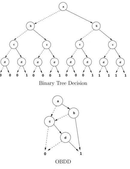
An OBDD has two terminal vertices labeled by 0 and 1, representing the truth value of the formula, respectively, false and true. For every truth assignment to the boolean variables of the formula, there is a corresponding path in the OBDD from root to a terminal vertex. If the path ends in the terminal vertex labeled by 0, then the assignment does not satisfy the formula, and conversely, if the terminal vertex labeled by 1 is reached, then the formula is satisfied by the assignment. Figure 2.6 illustrates an OBDD for the boolean formula (a∧b)∨(c∧d) compared to a Binary Decision Tree for this same formula.
OBDD, however, has drawbacks. In our approach, the most significant is related to the the variable ordering. Given a boolean formula, the size of the corresponding OBDD is highly dependent of the variable ordering. The OBDD can grow from linear to expo-nential to the number of variables of the formula. In addition, the problem of choosing an variable order that minimize the OBDD size is co NP-complete [17]. Despite the existence of heuristics to automatic ordering the variables, sometimes is necessary to order them manually.
2.2.2
The Model
a
b
c
d
c
d d
b
c
d d
c
d d
d
0
0 0 1 0 0 0 1 0 0 0 1 1 1 1 1
Binary Tree Decision
a
b c
d
0 1
OBDD
Figure 2.6: Binary decision tree (on top) and a correspondent OBDD (below) for the boolean formula (a∧b)∨(c∧d). The dashed arc is taken when var(v) = 0. The solid arc is taken whenvar(v) = 1.
if the model has three boolean propositions a, b, and c, then (a = 1 b = 1 c = 1), (a = 0 b = 0 c = 1), and (a = 1 b = 0 c = 0) are possible states. The symbolic representations of these states are (a b c), (a b c), and (a b c), respectively, where a means that this variable is true in the state anda means that this variable is false.
care true. Because symbols are used to represent states, algorithms that use this method are called symbolic algorithms.
a
b
c
a’
b’
c’
a b c
a b c
Figure 2.7: Example of a transition and its symbolic representation.
Transitions can also be represented by boolean formulas. A transition s → t is repre-sented by using two distinct sets of variables, S for the current state s and T for the next state t. Each variable in S has exactly one correspondent variable in T. For instance, if there are variablesa, b, c∈S, then there are variables labeled asa′, b′, c′ ∈T. Letfs be the formula associated with the statesandftbe the formula associated with the statet. Then, the transitions →t is represented by the formula fs∧ft. For example, a transition from the state (a b c) to the state (a b c) is represented by the formula¬a∧¬b∧¬c∧¬a′∧b′∧¬c′, as illustrated in Figure 2.7. The meaning of this formula is the following: there exists a transition from states to statet if and only if the substitution of the variable values fors, in the current state variables, and of those oft, in the next state variables, yieldstrueto the formula. The transition relation of the whole system is constructed from the disjunction of all transitions in the graph.
In the same way as boolean formulas can represent sets of states, they can also rep-resent sets of transitions. Symbolic Model Checking (SMC) takes advantage of this fact by representing sets of transitions using BDDs. The BDD representation can group sets of transitions into a single formula, which often significantly reduces the size of the final representation.
2.2.3
Search Algorithms
In [17], Bryant presents efficient algorithms to execute basic operations over boolean formulas. The time complexity of these algorithms is proportional to the size of the OBDD being manipulated. To our approach, our primary interest is the MIN algorithm [22], that traverses the SMC state transition graph, in a breadth-first search way, looking for the minimum path (number of arcs) between two specific states.
that are reachable fromS by paths of increasing length using a forwards search algorithm. Intuitively, the loop in the algorithm computes the set of states that are reachable fromF. If at any point, we encounter a state satisfying F, we return the number of steps taken to reach that state. Figure 2.8 illustrates this behavior, where the shaded area corresponds to the states reachable fromS visited at each step. In the algorithm presented in this figure, function T(S) returns the set of states that are successors of some state s ∈S; R and R′ represent sets of states.
S F
0:
S F
1:
S F
2:
S F
3:
proc MIN(S, F) i= 0;
R=S;
R′ =T(R)∪R;
while (R′ 6=R∧R′∩F =∅) do i=i+ 1;
R =R′;
R′ =T(R)∪R; if(R′∩F 6=∅)
then return i; else return ∞;
Figure 2.8: The MIN algorithm determines the minimum path between state s ∈ S and state f ∈F, in a breadth-first search way.
2.2.4
SMV - An OBDD Symbolic Model Checking Tool
SMV [66] is a symbolic model checker that implements all theorical features described above (Kripke model, CTL, and OBDD). SMV models a problem as a finite state machine. It is able to model synchronous and asynchronous problems. Non-determininsm is pro-vided and it can be used to model uncertaint events or unavailable modeling information. The properties about the model can be specified by CTL or LTL expressions. The input language provides code encapsulation (module) and passage of parameters among modules. The semantics of the assignment is similar to the assignment of data flow languages. An example of SMV program is presented in Figure 2.9. It is an an excerpt of a model relating to the microwave example presented in Section 2.1.3.
1 MODULE main
2 VAR
3 door : {opened, closed}; 4 cook : boolean;
5 setup : 0..5;
6 m : mw cell (setup, cook);
7 ASSIGN
8 init (door) := closed;
9 next (door) := {opened, closed}; 10 init (setup) := 0;
11 next (setup) := case
12 m.i = 0 : {0,1,2,3,4,5};
13 esac;
14 cook := ((door = closed) & (setup > 0));
15 SPEC!cook → EF m.cooking 16 SPECcook → AF m.cooking
17 MODULE mw cell (time, go) 18 VAR
19 i : 0..5;
20 ASSIGN
21 init (i) := time; 22 next (i) := case
23 go & (i> 0) : i - 1;
24 1 : i;
25 esac;
26 DEFINE
27 cooking := i >0;
ranging over lines 1 to 14, models a microwave user, setting the clock time for cooking a meal, and openning or closing the door of the microwave; the modulemw cell, ranging over lines 17 to 27, models the microwave cooking a meal. This SMV program also has two specifications in lines 15 and 16. These specifications are CTL properties that the SMV must verify.
TheVARsection of a SMV program determines the state space of the Kripke structure, since the state space is composed by all possible combinations of values of all variables of the model. Variables in SMV can be one of the following types: boolean;scalar; numeric, that is a range of integer numbers; or user defined. Array of variables are allowed. The lines 3 through 6 and line 19 present the variables declared for the microwave example.
The variabledoor(line 3) represents the door of the microwave. Its type is scalar what means that it can assume one of the values stated between the brackets, opened orclosed, in this case. The line 4 presents the declaration of variable cook. This variable is boolean and models the microwave state of cooking a meal. If cook is assigned to true, then the microwave is cooking. If cook is assigned to false, then the microwave is idle. The variable
setup in line 5 is numeric and its range varies from 0 to 5. This variable represents the possible set up time of the microwave for cooking a meal. Line 6 presents an example of user defined type. mrepresents the microwave action of cooking a meal, that is, it controls the passage of cooking time. Its behavior is defined by the modulemw celldeclared in lines 17 through 27.
The ASSIGN section of a SMV program defines the transition relation of the model. This section defines the initial and the next valuations of the program variables. Each valuation determines a state in the spcae of the model. In this program example, the ASSIGN section ranges over lines 7 through 14, in modulemain, and over lines 20 through 25, in modulemw cell. Theinit andnext declaration along these lines define, respectively, the initial value and the next value of the variables in the state space.
Line 8 states that the variable dooris initially assigned to closed. This means that the microwave door is always closed in the initial state of this model. Just considering this variable, if we have omitted this line, we would have two initial states, one state in which the value of variable door is opened, and another state in which its value is closed. The value of door in a next state can be opened or closed, as defined in line 9. This kind of assignement is non-deterministic.
to 0. Its value in a next state depends on the condition m.i = 0, in thecase construction. If m.i is greater than 0, it means that the microwave is cooking a meal, hence a new setup time is not allowed. Otherwise, if m.i = 0 yelds to true, the variable setup is assigned non-deterministically to any integer value between 0 to 5.
The variable cook indicates the condition for the microwave cooking a meal. cook
is assigned to true or false depending the result of the boolean expression stated in line 14. Finally, the variable i of module mw cell represents the clock time of the microwave. Initially, it is assigned to the value assigned tosetup, line 21. At each state,iis decremented by 1, if door is assigned to closed and setup is greater than 0, line 23. Note the relation between line 23 and line 14.
TheSPEC section of a SMV program is where we declare the properties (specifications) we want to be verified. In this model, we are interested to know if it is possible the microwave cooks a meal having its door opened or its clocktime set to 0 (see line 15). We are also interested in determining if the microwave really cooks a meal since all conditions for cooking are set (line 16).
SMV can be found fully documented at Carnegie Mellon University [79] or at Istituto per la Ricerca Scientifica e Tecnologica [26], where also can be freely downloaded.
2.2.5
Verus - A Symbolic Model Checking Tool for Real Time
Systems
Verus is a formal verification tool originally designed for time critical systems. It is based on CTL-OBDD-SMC technology and provides features specific time features, such as: deadline, delay, and priority. Verus also provides quantitative timing information about the model, such as: the minimum and maximum time interval between two events; the number of times an event has occurred in a given interval. These kind of informations are very important to detect system errors and/or optimize the system parameters.
The time in Verus is discrete, although some other tools adopt continuous time ap-proach [3, 52]. The continuous time demands a large state space to model a system, in general inhibiting the modeling of complex systems. Discrete time was project decision: it allows Verus to cope with very complex systems, with a state space of the order of 1030
1 boolean occurred;
2 alarm () {
3 boolean ring;
4 while (true){
5 if (occurred) ring = true; 6 else ring =false;
7 wait (1);
8 }
9 }
10 event () {
11 while (true){
12 occurred = select{false, true};
13 wait (1);
14 }
15 }
16 spec
17 AG (occurred–> AF alarm.ring);
Figure 2.10: A Verus program that models a non-deterministic event and its respective alarm.
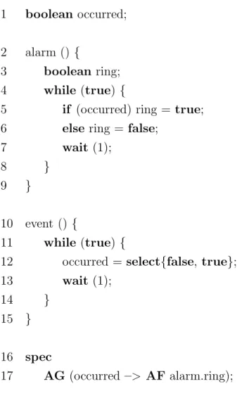
The Verus modeling language is similar toC language. This language paradigm is well known by the majority of designers and generally minimizes training. To present the Verus language, we will model a non deterministic event and an alarm (that rings when the event occurs). A Verus program relating to this scenario is presented in Figure 2.10.
This program presents two functions: alarm and event. Each Verus function models an independent process. The function alarm is declared over lines 2 through 9. It models an alarm that rings every time its associate event occurs. The function event models a non-deterministic occurrence of a certain event, and it is declared over lines 10 through 15. As we can see the functionmain is not mandatory.
Verus isinteger.
The functionalarmmodels an alarm that rings as soon as an event occurs. The boolean variable ring at line 3 models the ringing of the alarm. If this variable is true then the alarm is ringing. The function alarm loops forever assigning ring according to the value of
occurred. If occurred is true, this means that the event has occurred, then ring must be set to true. The alarm will keep on ringing until the event be ceased, that is, the variable
occurred be set to false. The variable occurred is assigned by the function event. This function loops forever assigning occurred non-deterministically to true or false (line 12).
The passage of time in the model is implemented by the wait statement, lines 7 and 13. This statement is responsible for creating the states of the model space. The functions of a Verus program can only perceive the new values of the program variables after wait statements.
Lines 16 and 17 present the specification of a property that Verus must verify. The property of line 17 informally speaking specifies that “everywhere in the model (AG) that event occurs (that is, the variable occurred is true), always in the future (AF) the alarm will ring (that is, the variablealarm.ring is true)”.
Symbolic Model Checking over a
Video on Demand System
The development of new technologies for high bandwidth networks, wireless commu-nication, data compression, and high performance CPUs has made it technically possible to deploy sophisticated infrastructures for multimedia applications [44, 80]. This type of infrastructure opens up opportunities for exploring multimedia applications such as qual-ity audio and video on demand (from home), virtual realqual-ity environments, digital libraries, and cooperative design. Figure 3.1 illustrates an infrastructure for such applications.
´ Wireless Link
´ PC
set-top-box TV and SERVER
Client Mobile
Network High Bandwith
Figure 3.1: Overall architecture for a video service.
at the server and client machines, and on the performance at the multimedia server. All these delays will determine the number of clients a VOD server can cope with at the same time.
A VOD server is quite distinct from conventional servers, such as database and Web servers, which do not have to take into account strict time constraints. In a VOD server, failure to meet the time application constraints will certainly lead to user dissatisfaction and consequently to risks of commercial failure. Further, to be cost effective a VOD server must present good performance (which is usually measured as the number of users which can be served simultaneously).
By the time we have been studying Verus the ALMADEN project was in course. AL-MADEM was a project financed by the Brazilian Ministry of Science and Technology, whose main purpose was the research about applications and algorithms for high perfor-mance multimedia networks. One of the products of this project was the ALMADEM-VOD server [69], whose prototype was operational, but without any formal evaluation about its performance bounds.
This chapter describes our work in the ALMADEM project, in determining the perfor-mance bounds of the ALMADEM-VOD server. We describe the ALMADEM-VOD server and its respective Verus model. We also describe the verification of this model and the min-imum (in the worst case) and the maxmin-imum number of clients (in the best case) determined by Verus.
3.1
The ALMADEM-VOD Server
The fundamental premise in the development of the ALMADEM-VOD server is that it should use only off-the-shelf low cost components, as also done in [44, 70, 80]. As a result, the server was implemented on a PC-based platform running the Linux operating system. To fulfill the real time requirements of the video application, the operating system was adapted in specific points such as the disk access and process scheduling routines.
as UDP messages. This software organization corresponds to the ALMADEM-VOD video server, and is illustrated in Figure 3.2.
STORAGE
DISK NETWORK
NETWORK 1
2 3
N BUFFER
thread priority=3 thread priority=2
thread priority=1
CLERK
Figure 3.2: Software architecture of the video server.
Two data structures and three separate processes are distinguished. The data structures are called storage and buffer. The processes (implemented as POSIX threads) are called disk, network, and clerk. To ensure proper timing in the scheduling of these threads, we rely on one of the real time scheduling policies available with the Linux operating system. We use the SCHED FIFO policy which implements a first-in-first-out scheduling scheme with static priorities. In this policy, the priority number of a thread is direct proportional to the system priority. Despite its simplicity, this scheme works quite well if the machine is dedicated to the video server task (i.e., we run the video server in run level 1).
The storage structure is composed of secondary or tertiary devices and is used to hold the collection of films available to the users. The current implementation of the ALMADEM-VOD server considers only secondary devices in the form of conventional SCSI-2 [78] disks of 4G bytes each. The disks store the films encoded and compressed in MPEG-1 [67] format. Each film is divided in blocks which are retrieved for delivery to the client machine. In its simplest implementation, which is adopted in this study, the ALMADEM-VOD server considers a contiguous layout of films on disk. In this layout, all blocks of a same film are stored contiguously on disk. More sophisticated layout schemes, involving striping techniques [10, 27], region-based allocation [46], and randomized place-ment [76], have been discussed extensively in the literature but are not the focus of this work.
The network thread is responsible for taking the blocks of film from the buffer and shipping them across the network. It is scheduled whenever the disk thread is blocked at the disk driver waiting for a disk access to complete.
The thread namedclerklistens at a TCP port for the requests from the client machines. Such requests might come from new clients or from a current client which requests, for instance, apausein the exhibition. Once it detects a client request, this thread passes the information to an admission control routine for proper scheduling. If the server is saturated (i.e., it is currently serving a maximum number of clients), a request for a new stream is not scheduled and a denial message is sent to the respective client.
The disk thread is responsible for reading the data from the secondary storage and storing them at the buffer area. To avoid delays introduced by the operating system (which we cannot control), disk accesses are performed through direct access functions which communicate directly with the SCSI controller device. For each active client, a separate block (which is composed of several MPEG frames) of (average) size B bytes is read, passed to the buffer area, and from there shipped (by the network thread) to the corresponding client machine. While that client consumes the frames in that block, other clients can be attended to. This cyclic scheduling process is repeated with a fixed time period equal to T, as illustrated in Figure 3.3. To implement this fixed time period, the diskthread monitors the Real Time Clock (RTC) device in the Linux kernel.
0 0 0 1 1 1 00 00 00 11 11 11 00 00 00 11 11 11
T
ST
ZB
B
B
t
s
t
r
t
s
t
r
t
s
t
r
1 2 3
T
Figure 3.3: Service cycle with a duration of T seconds. ts accounts both for seek and rotational delay times.
time. Thesleeping timeTz is the portion of the service cycle in which no clients are served. Such sleeping time is necessary because, to avoid buffer overflow at the client machine, the server does not attend a same client twice in a service cycle. The ratio Ts/T defines the occupation of the service cycle. Larger the occupation of the service cycle, higher is the load in the system.
In the ALMADEM-VOD server (as seen in Figure 3.3), the transfer time can vary from one film to another because the block sizes, though constant for a same film, differ from one film to another. The reason is that the coding scheme might vary from one film to another (for instance, a film might be encoded for a smaller window size) and that the compression rate is not constant across various films. The important detail is that, in the ALMADEM-VOD server, any block of any film is composed of roughly a same number of frames, which defines the duration of the service cycle. To exemplify, consider that each client consumes frames at the typical rate of 30 fps (frames per second). Then, if each block sent to a client includes 30 frames, the value ofT is 1 second to avoid interruption in the continuous display of the film at the client machine. If each block includes 120 frames, then the value ofT is 4 seconds.
To simplify the implementation, the ALMADEM-VOD server uses a Constant Data Length (CDL) block instead of a Constant Time Length (CTL) block [80]. The length of the blocks in which a given film is divided is determined by the maximum consumption rate at the client. This ensures smooth display at the client machine. However, buffer overflow might occur at the client because the rate of arrival exceeds the average consumption rate. To avoid this problem, the client sends a pausemessage to the server whenever it detects that its buffer is filling up.
LetRci be the rate (in bytes per second, or Bps) with which the ith client consumes a block of data. Further, let Bi be the size (in bytes) of the blocks of data for theith client, as indicated in Figure 3.3. Then, the periodT is given by
T = Bi
Rci (3.1)
Additionally, let Rd be the transfer rate of the disks in our secondary storage and let N be the maximum number clients which can be served in a cycle. We can then write
N X
i=1
Bi = (T −N ts)Rd (3.2)
By substituting equation (3.1) into equation (3.2), we obtain
N = T ts 1−
N X
i=1
Rci Rd
!
Equation 3.3 shows that the maximum number of clients in the system is a direct function of the ratioPN
i=1 Rci/Rd and thus, that the sum of all rates Rci must be smaller than the
disk transfer rateRd. Furthermore, the average block size (which determines the duration of the cycle service) must be large enough to provide an amortization of the time wasted with seek operations. In fact, a small average block size reduces the value ofT making the fractionT /tssmaller. This implies that the fraction of time available in a cycle for actually reading data from disk is smaller. This leads to a reduction in the maximum number of clients which can be attended simultaneously.
10 15 20 25 30 35 40 45 50 55 60 65 70 75 80 85
0 1 2 3 4 5 6 7 8 9 10
Service Cycle Occupation Ts/T (%)
T
Figure 3.4: Service cycle occupation in the ALMADEM-VOD server for periods varying from 1s to 9s. The number of clients in the system is 20.
Amortizing seek time (through an increase in the service cycle) is critically important because it improves server performance (in terms of the maximum number of clients which can be served). However, an excessive increase in the service cycle is counter-productive because it implies in an excessive latency — the time a new user waits to be served. This is because new users are only served in the cycle which initiates following their arrival. Additionally, large service cycles require larger memory buffers at the server and at the client machines.