www.hydrol-earth-syst-sci.net/15/819/2011/ doi:10.5194/hess-15-819-2011
© Author(s) 2011. CC Attribution 3.0 License.
Earth System
Sciences
Examination of homogeneity of selected Irish pooling groups
S. Das and C. Cunnane
Department of Engineering Hydrology, National University of Ireland, Galway, Ireland Received: 1 July 2010 – Published in Hydrol. Earth Syst. Sci. Discuss.: 30 July 2010 Revised: 15 February 2011 – Accepted: 16 February 2011 – Published: 9 March 2011
Abstract. Flood frequency analysis is a necessary and im-portant part of flood risk assessment and management stud-ies. Regional flood frequency methods, in which flood data from groups of catchments are pooled together in order to enhance the precision of flood estimates at project locations, is an accepted part of such studies. This enhancement of pre-cision is based on the assumption that catchments so pooled together are homogeneous in their flood producing proper-ties. If homogeneity is assured then a homogeneous pool-ing group of sites lead to a reduction in the error of quan-tile estimates, relative to estimators based on single at-site data series alone. Homogeneous pooling groups are selected by using a previously nominated rule and this paper exam-ines how effective one such rule is in selecting homogeneous groups. In this paper a study, based on annual maximum se-ries obtained from 85 Irish gauging stations, examines how successful a common method of identifying pooling group membership is in selecting groups that actually are homoge-neous. Each station has its own unique pooling group se-lected by use of a Euclidean distance measure in catchment descriptor space, commonly denoteddij and with a
mini-mum of 500 station years of data in the pooling group. It was found thatdij could be effectively defined in terms of
catchment area, mean rainfall and baseflow index. The study then investigated how effective this selected method is in se-lecting groups of catchments that are actually homogenous as indicated by their L-Cv values. The sampling distribu-tion of L-CV (t2) in each pooling group and the 95% con-fidence limits about the pooled estimate oft2 are obtained by simulation. Thet2values of the selected group members are compared with these confidence limits both graphically and numerically. Of the 85 stations, only 1 station’s pooling group members have all theirt2values within the confidence
Correspondence to:S. Das (samirandas@gmail.com)
limits, while 7, 33 and 44 of them have 1, 2 or 3 or more,t2 values outside the confidence limits. The outcomes are also compared with the heterogeneity measures H1 and H2. The H1 values show an upward trend with the ranges oft2values in the pooling group whereas the H2 values do not show any such dependency. A selection of 27 pooling groups, found to be heterogeneous, were further examined with the help of box-plots of catchment descriptor values and one particu-lar case is considered in detail. Overall the results show that even with a carefully considered selection procedure, it is not certain that perfectly homogeneous pooling groups are iden-tified.
1 Introduction
It is widely accepted that a short annual flood (AM) series is inadequate for the estimation of design floods of large return periods. Regionalization (FSR, 1975), i.e. pooling analysis (FEH, 1999), is one of the possible methods used to provide a framework for design floods. In pooling analysis flood data are pooled from other gauging stations that possess similar hydrological behaviours to the at-site station. A very com-mon way to implement regional/pooling is the index flood method proposed by Dalrymple (1960). The estimation of QT, T-year flood, based on this approach involves derivation
of a growth curve which shows the relation betweenXT and
the return periodT whereXT=QT/QIandQIis the index flood at the site of interest. Generally the mean (FSR, 1975) or median (FEH, 1999) of the at-site AM flood series is taken as the index flood. It is assumed that theXT−T relation is
However very recently Kjeldsen and Jones (2009) have ap-proached this in a different way.
An examination of homogeneity is normally used to assess whether a proposed group of sites is homogeneous or not. Examination of the homogeneity of regions/pooling groups is usually based on a statistic that relates to the formulation of a frequency distribution model, e.g. the coefficient of vari-ation, CV (Wiltshire, 1986; Fill and Stedinger, 1995) and/or skew coefficient,g, their L-moment equivalents (Chowdhury et al., 1991; Hosking and Wallis, 1997) or of dimensionless quantiles such as the 10-year event (Dalrymple, 1960; Lu and Stedinger, 1992). Hosking and Wallis (1993, 1997) proposed homogeneity tests based on L-moment ratios such as L-CV alone (H1) and L-CV and L-skewness jointly (H2) which are widely used in flood frequency analysis although the for-mer one is recommended by these authors for having better power to discriminate between homogeneous and heteroge-neous regions. Very recently, a similar conclusion has been drawn by Viglione et al. (2007) when they compared sev-eral homogeneity tests. They stated that the H1 test is ahead of all others when the L-skewness is lower than 0.23. They further concluded that the H2 as a homogeneity test lacks power. These findings certainly indicate that the heterogene-ity among the sites in a group is mainly due to variations in the sample L-CVs. However, one of the main assumptions of these tests is that the true regional distribution is kappa. For that reason and others Hosking and Wallis (1997) recom-mended that though the heterogeneity statistic is constructed like a significance test it should not be used in that way. They, Hosking and Wallis (1997, p. 70), further stated that “. . . a significance test is of doubtful utility anyway, because even a moderately heterogeneous region can provide quantile es-timates of sufficient accuracy for practical purposes. Thus a test of exact homogeneity is of little interest.” In this paper a graphical way of examining the homogeneity of a pooling group is presented which is based on L-CV , i.e. t2. The main idea behind the approach is the comparison of the vari-ability oft2from each site in the pooling group with that ex-pected (un-weighted average pooledt2) supposing the differ-ences between sites to be due to sampling error. The pooling groups are identified by the Region of Influence (ROI) ap-proach. The population distribution is GEV (withk=−0.05, k= 0.0,k= +0.03), rather than Kappa as suggested by Hosk-ing and Wallis (1997), and was based on the GEV’s descrip-tive ability of the annual maximum data series of Ireland.
The outline of the paper is structured as follows: the next section describes the procedure used to obtain growth factors and flood quantiles in the context of flood frequency pooling analysis. This is followed by a description of procedures to select pooling variables for similarity distance measure (dij)
in the context of formation of pooling groups using the ROI approach. A graphical way of examining homogeneity of pooling groups obtained by the ROI approach is then pre-sented. Then the analysis of the examination procedure is summarised and finally a selected number of heterogeneous
pooling groups are reviewed with the help of Box-plots of catchment descriptors.
2 Estimation of pooled growth factors and flood quantiles
The growth factorXT is the factor which when multiplied
by the index floodQI , gives the flood magnitude of return
periodT,QT, as in Eq. (1)
QT = QI ×XT (1)
The relationship betweenXT andT is often referred to as the
growth curve. When a growth curve is obtained by pooling the information from sites of a pooling group, it is called the pooled growth curve. Qmed is used as the index flood in this study where Qmed is the median of the annual maximum series.
In this study the pooled growth curve is obtained using the approach based on the method of moments. The L-moments developed by Hosking (1990) are based on proba-bility weighted moments (PWMs) introduced by Greenwood et al. (1979). With this approach the derivation of a growth curve in a pooling group involves the following key steps:
1. computation of at-site and pooled L-moment ratios 2. selection of a suitable form of distribution and
estima-tion of its parameters by the method of L-moments. moments are calculated and then the dimensionless L-moment ratiost2andt3are calculated for each site. Pooled L-moment ratios for the target site,i, are then computed using the following equation:
t(i)R =
PM
j=1wij t(j )
PM
j=1wij
(2)
wheret(j )is the L-moment ratio (eithert2ort3) for thej-th most similar site andwijis a weighting term.
Weights can be related to a site’s record length and/or a site’sdij values. Recently a more complex way of assigning
weights is proposed by Kjeldsen and Jones (2009) although they state that only a little has been gained in the flood esti-mation procedure using the new approach. In this studywij
The Generalised Extreme Value (GEV) has been selected as the pooled distribution function. The selection of the GEV distribution is explained in Sect. 4. The values t2R,t3R are equated to expressions for these quantities written in terms of the distribution’s unknown parameters (expressed in dimen-sionless form) and the resulting equations are solved for the unknown parameter values. The dimensionless GEV growth curve (XT) is defined by two parameterskandβ:
XT = 1 +
β
k (ln 2)
k −
ln T T −1
k!
(3) whereT is the return period.
The two parameterskandβare estimated from the sample L-CV,t2, and sample L-skewness,t3, as follows (Hosking and Wallis, 1997)
k = 7.8590c+2.9554c2 (4)
in which
c = 2
3+t3 − ln 2
ln 3 (5)
β = k t2
t2 Ŵ (1 +k) − (ln 2)k +Ŵ (1 +k) 1 −2−k (6)
whereŴdenotes the complete gamma function.
3 Formation of pooling groups using Region Of Influence (ROI) approach
The Region of Influence (ROI) approach of formation of a pooling group is considered to be the most appropriate and meaningful way of delineating a pooling group. The tech-nique developed by Burn (1990), involves the identification of a region of influence i.e. a separate pooling group for each gauging station in a region. The identification of a pooling group consists of selecting stations that are hydrologically similar to the site of interest. Similarity is measured gener-ally by a Euclidean distance measure in catchment descriptor space.
The effective identification of a pooling group in a ROI approach is governed by two important criteria: the choice of appropriate site descriptors as pooling variables and the size of a group in terms of number of sites and station years included. Burn (1990) investigated a number of options to determine a threshold value based on thedij values to define
a cut-off for the inclusion of stations in the ROI method for a target site. However, a more practical way of choosing an appropriate size of a pooling group was presented by FEH (1999). They investigated a range of pooling group sizes and decided on adoption of the 5T rule, namely that the total number of station years of data to be included when estimat-ing theT year flood should be at least 5T. The adoption of such a rule was a compromise. If too few stations are in-cluded the precision of theQT estimate is sacrificed whereas
if far too many stations are included then the assumption of homogeneity may be compromised. Hosking and Wallis (1997) however show that a small departure from homogene-ity can be tolerated so that having too few stations included may be less desirable than having slightly too many. They also suggested not to use more than 20 sites in a group as little gain in the accuracy of quantile estimates is obtained by using more than about 20 sites in a group. Recently, Kjeldsen and Jones (2009) found that a fixed pooling group consist-ing of 500 station years performed well for a range of return periods. In relation to identifying site descriptors as pooling variables, careful consideration is necessary as to which form of catchment descriptors are to be used in a ROI method of pooling analysis. In the next subsection an investigation of selecting pooling variable for the Irish case is described in detail.
3.1 Choice of catchment descriptors on effectiveness of ROI distance measures
The general form of the similarity measure used for selecting members of a pooling group is defined by
dij =
v u u t
n
X
k=1
Wk Xk,i −Xk,j
2
(7)
wheredij is the weighted Euclidean distance from sitej to
sitei;nis the number of attribute variables;Xk,iis the value
of thek-th variable at thei-th site andWk is the weight
ap-plied to attribute k, reflecting its relative importance. The subscripti denotes the subject site and the subscript j de-notes thej-th pooled site.
In choosing a distance measuredij a decision has to be
made about which catchment descriptors are to be included in the distance measure and what weightings are to be ap-plied to them and whether logarithms or other transforma-tions are to be used. The FEH (1999) provided a number of useful maxims for choosing a distance measure. It rec-ommended not to use at-site flood statistics (e.g. CV,g) as pooling variables because this might well result in groups consisting of sites that have experienced similar floods in re-cent history. Neither could such site flood statistics be used for ungauged catchments. Seasonality of the flood response (e.g. timing and regularity of flood events) has also been con-sidered (Burn, 1997; Cunderlik and Burn, 2006) as a simi-larity measure. Seasonality statistics are obtained from ob-served flood series. Therefore, a similarity measure based on these could not be used for ungauged sites, without addi-tional assumptions.
For Irish conditions two sets of catchment descriptors have been selected as potential pooling variables:
– on the assumption that homogeneity is strongly depen-dent on CV or L-CV, those catchment descriptors that could predict L-CV best were identified and a selection of these were used to formdij. This approach is along
the lines outlined by Kjeldsen and Jones (2009). For selecting the final set of pooling variables, FEH used pooled uncertainty measure (PUM) which is a weighted av-erage of the squared differences between each at-site growth factor and the pooled growth factor measured on a logarith-mic scale. In this part of the study a simulation procedure is used for this purpose because far fewer stations (85) than the 602 stations used for the UK study were available. The first objective is to find which combinations of FEH descriptors, which are listed in Table 2, lead to pooling groups which are most effective at exploiting the information about the flood distribution contained in the pooling groups.
The simulation procedure uses the GEV distribution for data generation which is considered to be representative of what is appropriate in Irish conditions. Hosking and Wal-lis (1997, p.93) suggested not to use the observed sample L-moment ratios as the population L-moment ratios of the simulated region because this would yield a simulated re-gion that has much more heterogeneity than the actual data. Castellarin et al. (2001) addressed the issue by using a region of influence approach to estimate the at-site population val-ues oft2andt3. A similarity measure based on at-site flood statistics is used to form a group of sites for a subject site and its population values oft2 andt3are considered as the cor-responding pooled estimate oft2andt3for the group. Later, Ga´al et al. (2008) adopted this approach in their study. A similar kind of approach is used here with a similarity mea-sure defined as
δij =
s t2
,i −t2,j
σt2
2
+
t3
,i −t3,j
σt3
2
(8) which is independent of the descriptor variables being con-sidered in Table 2. A pooling group is formed for each site using Eq. (8) and the pooledt2 andt3 are estimated using Eq. (2). The estimated pooled values oft2andt3 are then used as population values for each site in step 2 of the sim-ulation procedure. The simsim-ulation procedure does not con-sider the implications of intersite correlation among sites in a pooling group because it was found by Hosking and Wallis (1997, p.127) to be of very little consequence. The steps of the simulation procedure for selecting variables are described as follows.
1. The gauging stations in the subject site’s pooling group are identified using thedij values of Eq. (7) for a set of
catchment descriptors having a minimum of 5T station years of data in the pooling group.
2. Random samples are drawn from GEV populations for the subject site and for each site in the pooling group.
For each site the sample size is taken as being equal to the length of the observed historical record at the site and the parameters are estimated from the sitet2andt3 values obtained using the procedure described above, as in Castellarin et al. (2001) and Ga´al et al. (2008). 3. Thet2andt3values are obtained for each sample in the
pooling group and the average of these is calculated to represent the pooledt2andt3values.
4. The pooledt2andt3values are then used to determine the pooling group’s GEV growth curve parameters k andβusing Eqs. (4) and (6).
5. The subject site’sXˆT value is calculated forT= 50 and
100 years respectively using Eq. (3).
6. Steps 2 to 5 are repeated 10 000 times to provide 10 000 values ofXˆT and the RMSET and BIAST are
calculated for the subject site by the following equa-tions:
RMSET[%]=
1 M M X i=1 v u u t1 S S X s=1 ˆ Xi,sT −XTi
XTi
!2
×100 (9)
BIAST[%]=
1 M M X i=1 1 S S X s=1 ˆ XTi,s−XiT
XiT
!
×100 (10)
whereXˆi,sT is the estimated T-year growth factor at a siteiat thes-th repetition;XTi is the assumed trueT -year growth factor at sitei;Mis the number of sites in the pooling group andSis the number of repetitions. RMSET and BIAST defined in the simulation procedure
has been evaluated at 50 and 100-year return periods for each site. The eight combinations listed in Table 2 of the four variables have been tested based on RMSET
(primar-ily) . In all, 85 stations have been considered for the study. The data sets that have been used in the study are summa-rized in Table 1. For each of these sites, a pooling group was selected from the 85 stations. Initially in the simula-tion procedure all weightsWk in Eq. (7) were set to unity.
Fig. 1.Box-plot of RMSE of growth factors corresponding to 100 yr return periods for different sets of catchment descriptors used in defining the distance measuredij. Each Box-plot gives the percentiles for the frequencies 0.05, 0.25, 0.5, 0.75, 0.95.
Fig. 2.Values of BIAS for the analysis summarised in Fig. 1.
the most suitable set of pooling variables for Irish conditions. However, if there is also a desire to incorporate another phys-ical catchment effect then the BFI could be included with these two. While inclusion of just one or two catchment de-scriptors may indeed be best, there is an intuitive attraction in also representing some descriptor of catchment response even at the cost of a small apparent loss in effectiveness. This could be of relevance in engineering investigations where differences in catchment behaviour are considered of impor-tance by the investigator. An extension to this investigation with varying values of weightsWk in Eq. (7) was also done,
particularly for the set of variables of lnAREA, lnSAAR and BFI but the results of all variations examined are not reported in detail here. An automatic search procedure was not used but it was found, by trial and error, that the weights 1.5, 1.0 and 0.1 for lnAREA, lnSAAR and BFI respectively gave RMSE100= 15.22 and RMSE50= 12.81 which offer small improvements on the Wk= 1.0 values used in the
calcula-tions for the set of variables of lnAREA, lnSAAR and BFI. The trial and error approach involved assigning a selection of weights, varying from 0 to 3, to each of the quantities, i.e. lnAREA, lnSAAR and BFI.
Table 1.Summary of AMF data sets used in the study.
Number of stations 85
Shortest record length 17 Longest record length 55 Mean record length 36.5 Number of AMF events 3213
Table 2. Variation in the mean RMSE corresponding toT= 100 and 50 for different sets of pooling variables: variables as used in FEH (1999).
Variables used in model RMSE100% RMSE50%
lnAREA (lnA) 15.13 12.47
lnAREA, nSAAR (lnA + lnS) 15.11 12.77 lnAREA, lnSAAR, BFI (lnA + lnS + B) 15.52 13.22 lnAREA, lnSAAR, BFI, FARL (lnA + lnS + B + F) 15.57 13.20
lnSAAR (lnS) 15.27 13.23
BFI (B) 15.97 13.83
lnAREA, BFI (lnA + B) 16.21 13.44
lnAREA, lnSAAR, FARL (lnA + lnS + F) 15.54 12.78
% of catchment area affected by arterial drainage improve-ments. These descriptors were identified from a pool of twenty five catchment descriptors made available by the Irish Office of Public Works. TheR2value of the best available model is a modest 29%.
These identified catchment descriptors were also assessed by the above simulation procedure. The RMSET values for
T= 50, 100 are listed in Table 3 for six combinations of the three variables. The set of two variables, lnMSL and ARTDRAIN, and the set of the single variable lnMSL per-formed best in terms of providing the lowest RMSE100% val-ues.
Both approaches described above provide similar out-comes in terms of RMSE100%. This may be partly due to the relatively weak relations identified for predicting L-CV (R2= 0.29). A regression of L-CV on the other set’s catch-ment descriptors (AREA, SAAR, BFI, FARL) also yields a weak relation for predicting L-CV (R2= 0.21). Since both sets of catchment descriptors can predict L-CV only in a weak manner, and both approaches are similar in RMSE it is concluded that neither approach is clearly superior to the other.
4 Procedure for examination of homogeneity
A homogeneity test is used to assess whether a proposed group of sites is homogeneous or not. A homogeneous group of sites leads to a reduction in the error of quantile estima-tors relative to estimaestima-tors based on single at-site data series alone which is the main goal of a regional flood frequency analysis. A homogeneity test was introduced by Dalrymple (1960). Other tests were introduced by Wiltshire (1986), Lu and Stedinger (1992), Fill and Stedinger (1995) and Hosking and Wallis (1993, 1997).
A simulation procedure, using graphical presentation of key results is applied in this study to examine homogene-ity of pooling groups that were formed using the ROI tech-nique. GEV distributions with 3 different shape parame-ter values (k=−0.05, k= 0.0 (EV1),k= +0.03) are used in
Table 3. Variation in the mean RMSE corresponding toT= 100 and 50 for different sets of pooling variables: variables that predict L-CV best.
Variables used in model RMSE100% RMSE50%
lnMSL 15.12 12.59
lnMSL, FORMWET 15.19 12.82
lnMSL, FORMWET, ARTDRAIN 15.23 12.81
FORMWET 16.89 15.41
ARTDRAIN 15.80 13.97
lnMSL, ARTDRAIN 15.09 12.80
the simulation procedure. The GEV, and its special case the EV1, have a history of usage in Ireland since publica-tion of the Flood Studies Report (FSR, 1975, p.173–174, Ta-ble 2.38, Fig. 2.14, Vol. I). More recently, a national study sponsored by the Office of Public Works, Dublin, based on annual maximum flood data of 110 stations, with average length of record 37 years and with a quarter of them between 50 and 55 years, has indicated that GEV and EV1 distribu-tions are suitable parents for the majority of Irish flood series (Das, 2010, Ch. 3). This conclusion is based on visual ex-amination of probability plots and numerical scores assigned to them, on classical goodness of fit tests and on L-Moment Ratio diagrams, such as Fig. 10 which shows that GEV/EV1 looks more suitable as a parent than other 3-parameter dis-tributions tested such as Generalised logistic and Lognor-mal 3. While the 4 parameter Kappa distribution has been recommended by Hosking and Wallis (1997) as a parent for simulation studies, this choice was sometimes found to be problematical because of numerical difficulties and estima-tion failures during the parameter estimaestima-tion process and as a result GEV was selected as parent distribution in this study.
The steps of the simulation procedure are as follows: 1. The gauging stations in the subject site’s pooling group
are identified usingdij values obtained by the following
equation having a minimum of 500 station years of data in the pooling group and satisfying the 5T rule for the 100 year quantile.
dij = (11)
s
1.5
lnA
i−lnAj σlnA
2 +
ln SAARi−ln SAARj σln SAAR
2 +0.1
BFIi−BFIj σBFI
2
The weights 1.5, 1.0 and 0.1 are those reported in Sect. 3 above.
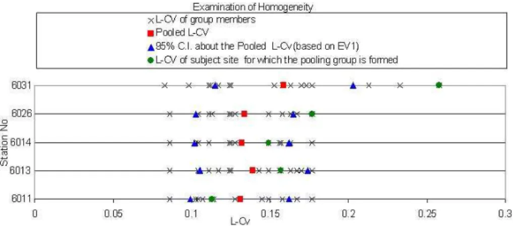
Fig. 3.Examination of homogeneity (EV1 case).
Table 4. Summary of events outside the confidence limits for 85 pooling groups.
events GEV EV1 GEV
outside (k=−0.05) (k= 0) (k= +0.03) the
CL (m)
No. of groups (%) No. of groups (%) No. of groups (%)
0 2 (2) 1 (1) 0 (0)
1 13 (15) 7 (8) 7 (8)
2 12 (14) 8 (9) 8 (9)
3 24 (28) 25 (29) 23 (27)
>3 34 (40) 44 (52) 47 (55)
3. Random samples are drawn from GEV distributions with 3 different shape parameter values (k=−0.05, k= 0.0 (EV1), k= +0.03) using the t2R as the popula-tion value to construct a 95% confidence interval for t2R. These population shape parameters, k=−0.05 , k= 0.0 (EV1) andk= 0.03, are selected in this context which correspond to L-skewness≈0.21, 0.17 and 0.15 respectively, this being the range relevant for Ireland. The sample size is taken as being equal to the aver-age record length of the observed historical record at the gauging sites and the parameter values are estimated from the value of thet2R. The 95% confidence interval is constructed assuming that the samplest2R values are normally distributed. While the L-CV values may not be perfectly normally distributed Viglione’s (Viglione, 2010) results show that the departure from normality is not severe for the range of L-CV and L-skewness val-ues that are observed in Irish conditions. Hence the nor-mality assumption was made in the calculation of con-fidence intervals.
4. The number of stations in the selected pooling group whoset2values fall outside the confidence interval (the attribute termed here asm) is counted and reported. It
Table 5. Summary of heterogeneity measure, H1 and H2 for 85 pooling groups.
Heterogeneity % of groups with % of groups with measure heterogeneity<2 heterogeneity<4
H1 5 22
H2 38 86
is also noted whether thet2of the subject site is outside the confidence limits (CL).
4.1 Analysis
The procedure described above is applied for each of the 85 stations. Each station had its own unique pooling group. The sample values oft2for the stations in the group,t2Rand the CL aboutt2Rare displayed in Fig. 3 for five stations. The summary statistics of the procedure are given in tabular form in Table 4. In addition to that the heterogeneity measures, H1 and H2, described in Appendix A, for each group is cal-culated and a summary of these measures is reported in Ta-ble 5.
The following observations and findings are obtained from the analysis.
1. Table 4 lists how many stations, mfall into the cate-gories of zero value outside the CL, one value outside the CL, 2 values outside the CL, 3 values outside the CL or more than 3 outside the CL. In all, for the case of EV1, only one station (1%) was in the first category while 52% of stations were in the latter category. This information in the form of proportion of values, m/N
Fig. 4. H1 plotted versus range of L-CV. Each point represents a pooling group.
Fig. 5. H2 plotted versus range of L-CV. Each point represents a pooling group.
values for GEV (k=−0.05) and GEV (k= +0.03) are broadly similar.
2. From Table 4, it is seen that as the shape parameter in-creases fromk=−0.05 to +0.03 the number of cases wherem >3 increases from 33 to 47.
3. In 27 groups (32% of groups) thet2of the subject site was outside the CL for the case of EV1. The corre-sponding numbers for the case of negative shaped GEV and for the case of positive shaped GEV are 27 and 28 respectively. All the 27 stations of the EV1 case were also in the latter cases.
4. Table 5 summarises the results of H1 and H2 for the 85 pooling groups. 22% of groups have a H1 value lower than 4.0. The percentage increases to 86% when the same criterion is set for H2 and that is very similar to what was found for the UK pooling groups (FEH, 1999, p. 176).
5. The range oft2values, maxt2–mint2, was calculated for the 85 pooling groups. The average range oft2for the 85 pooling groups was 0.11 with a minimum value
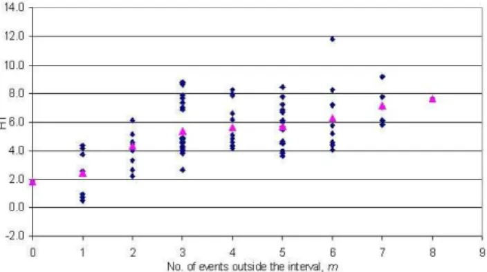
Fig. 6.H1 plotted versusm. Each point represents a pooling group.
of 0.06 and a maximum value of 0.18. Figure 4 shows a plot between H1 values and ranges of L-CV values for the 85 groups. The plot shows an upward trend, im-plying that a high H1 value can be expected when the t2values in a pooling group have a large range, which can be expected in the absence of homogeneity. A sim-ilar plot is drawn for H2 in Fig. 5, showing no obvious trend, implying that a low H2 value may be obtained for a pooling group which is in fact a heterogeneous group. 6. Figure 6 shows a plot between H1 andm. Different val-ues of H1 occur for a particularmvalue and that is rea-sonable as the memberships of the groups in those cases are different even though they may have some overlap. However, the average values, marked by triangles in the plot, show an increase of H1 withm, i.e. the higher the number oft2values of group members outside the CL, the higher the value of H1 that can be expected. If a H1 value less than 4.0 is considered as a good criterion for testing homogeneity, then in this approach it is required that fewer thanm= 2 values fall outside the confidence limit, i.e.m/N≤0.15.
Fig. 7.H1 plotted versusdij,max. Each point represents a pooling
group.
5 Investigation of selected heterogeneous pooling groups
The investigation has been carried out on those 27 cases where the pooling groups are heterogeneous and in which the t2of the subject site lies outside the confidence limits. The investigation mainly focuses on identifying any inappropri-ateness among group members that would cause the pooling groups to be heterogeneous. In this context, FEH (1999, 3, Fig. 16.9) documented a detailed review system, providing an example. That system mainly considers two attributes: (1) whether the subject site has any special qualities that need to be taken into account and (2) whether any of the pooled sites has catchment descriptors that are particularly different from those of the subject site. Sites in the pooling group can be investigated using several characteristics including at-site flood statistics and catchment descriptors. Statistics in a pooling group such as discordancy measure (Hosking and Wallis, 1997) and the distance measure (dij) can also be used
to investigate sites in the pooling group. In this part of the study, four catchment descriptors, namely, AREA, SAAR, BFI, FARL; and the distance measure (dij) are taken into
account in the investigation process. The first three of the catchment descriptors, AREA, SAAR and BFI,were already used for initial selection of sites for a pooling group. In the investigation procedure, sites are reviewed with the help of Box-plots and a summary table and in some cases, with the help of the ‘examination of homogeneity’ chart described in Sect. 4. Four Box-plots of catchment descriptors, such as AREA, SAAR, BFI and FARL, are constructed to show the subject site in the context of the pooling group. For each of these catchment descriptors, the placement of numerical values for sites in the pooling group is displayed against a backdrop of the relative frequency of the 85 sites considered in this study. This facilitates the identification of any partic-ularly inappropriate sites. In the summary table, statistical properties such ast2,t3anddij values of sites in a pooling
group are listed as shown in Fig. 9. The investigation pro-cedure for pooling groups of station no 6031 is described in detail as it serves as an example.
Fig. 8. mplotted versusdij,max. Each point represents a pooling
group.
An example: station no 6031 on the River Flurry
There are 17 sites in the pooling group of which eight, includ-ing the subject site, have values which fall outside the CL, thus indicating a strongly heterogeneous group. The hetero-geneity measures H1 and H2 for the group are 7.66 and 2.82 respectively. The examination of Box-plots in Fig. 9 reveals the catchment area of the subject site is small (46.2 km2) and it is very near to the 5 percentile mark on the Box-plot of AREA. The site is not positioned at the centre of the group of gauged catchments in the pooling group. There are 5 sites on the left of the subject site and there are as many as 11 sites on the right. The attribute certainly includes some sites that have large catchment area compared to the subject site. This may lead to dij values exceeding the value 1.0 in several
cases. Thedij values for the last three sites are around 1.3
and these sites are among the seven other sites that fall out-side the CL. The examination of the summary table on the right hand side of Fig. 9 shows that the subject site has large values of botht2andt3and that these are the largest among the group members. Hence, the conclusion can be drawn here that the pooling group in its present structure may not be ideal for that subject site 6031. Leaving out some sites at the bottom of the table might be considered in this context. The large number of sites, 17, in the pooling group is also a possible contributor to heterogeneity.
Fig. 9.Four Box-plots and a summary table for investigating a pooling group. The subject site is marked with a×. Small dots denote sites included in the pooling group. The underlying distribution of each catchment descriptor is shown in the Box-plots. Each Box-plot gives the minimum and the maximum value (+) and percentiles for the frequencies 0.05, 0.25, 0.5, 0.75, 0.95. The summary table lists record length,
t2,t3anddijvalues for a 100-yr pooling group for subject station 6031.
Fig. 10. L-moment ratio diagram for annual maximum flow for 110 Irish stations.
6 Conclusions
In the context of ROI pooling group based flood frequency estimation procedure, the most suitable form of distance measuredijfor Irish conditions was sought. The ROI method
with the suitably identified distance measure, Eq. (1), was used to form pooling groups for the subject sites. A simple graphical approach of examining homogeneity of the pooling groups was presented. The graphical approach compared the sampling variability of pooled estimates of CV with the L-CV of pooling group members. The approach also allowed the location of L-CV of the subject site to be viewed in the context of pooling group members, which is important in the
case of site specific pooling group. Most of the Irish pooling groups exhibited a degree of heterogeneity among the group members. A graphical approach of reviewing a heteroge-neous pooling group was also presented in this context. The following conclusions were obtained from the above studies: 1. It was found that the distance measuredij could be
sat-isfactorily defined in terms of lnAREA and lnSAAR but if there is a desire to incorporate another physical catch-ment effect then the BFI could be included with these two. Thedijcan also be defined in terms of lnMSL and
ARTDRAIN.
hydrologically similar; but in some cases the fulfillment of that condition does not guarantee that the pooling group is homogeneous.
Appendix A
Heterogeneity test measures
The heterogeneity test measures proposed by Hosking and Wallis (1997) are based on (1) L-CV alone (the H1 statis-tic) and (2) L-CV and L-skewness jointly (the H2 statisstatis-tic). These tests measures the sample variability of the L-moment ratios among the samples in the pooling group and compare it to the variation that would be expected in a homogeneous pooling group. The sample variability of the L-moment ra-tios is measured as the standard deviation of the at-site sam-ple L-moment ratios weighted proportionally to the sites’ re-spective record lengths. The measure of the sample variabil-ity based on L-CV alone, i.e.V1, and L-CV and L-skewness jointly, i.e.V2, are defined as
V1 =
"M X
i=1 ni
t2i −t2R2.
M
X
i=1 ni
#1/2
(A1) V2 = M X i=1 ni
t2i−t2R 2
+t3i−t3R 21/2
.XM
i=1
ni (A2)
where t2R and t3R are the group average of CV and L-skewness, respectively;t2i,t3i andni are the values of L-CV,
L-skewness and the sample size for siteiandMis the num-ber of sites in the pooling group.
Simulation is used to establish what “would be expected” of a homogeneous group. Some 500 homogeneous groups are generated using a four-parameter kappa distribution with L-moment ratio values equal to t2R, t3R, t4R and the at-site mean, L1 = 1, in order to obtain the expected mean value, µVj, and the standard deviation,σVj, of the variability
mea-sures for a homogeneous group.
The heterogeneity measuresHj are then estimated using
the expression below.
Hj =
Vj −µVj
σVj
, for j = 1,2 (A3)
Hosking and Wallis (1997) recommended using the H1 statistic over the H2 statistic as they found that the het-erogeneity measure based on V1 has better power to dis-criminate between homogeneous and heterogeneous regions. They suggested that a region is considered to be “accept-ably homogeneous” if H1<1, “possibly heterogeneous” if 1<H1<2, and “definitely heterogeneous” if H1>2. How-ever, the H2 statistic as the heterogeneity measure was adopted by FEH (1999) for testing the homogeneity of
pooling groups as both the L-CV and L-skewness are re-quired for fitting pooled growth curves with a Generalised Logistic (GLO) or a Generalised Extreme Value distribu-tion (GEV). FEH (1999) revised the heterogeneity criteria based on the H2 statistics, suggesting that if 2<H2<4, a re-gion could be considered as heterogeneous whereas if H2>4 it could be considered as strongly heterogeneous.
Acknowledgements. The authors would like to acknowledge the financial support made available by the Irish Office of Public Works. Comments and suggestions from two anonymous reviewers and from the editor, Francesco Laio are gratefully acknowledged.
Edited by: F. Laio
References
Burn, D. H.: Evaluation of regional flood frequency-analysis with a region of influence approach, Water Resour. Res., 26, 2257– 2265, 1990.
Burn, D. H.: Catchment similarity for regional flood frequency analysis using seasonality measures, J. Hydrol., 202, 212–230, doi:10.1016/S0022-1694(97)00068-1, 1997.
Castellarin, A., Burn, D. H., and Brath, A.: Assessing the effec-tiveness of hydrological similarity measures for flood frequency analysis, J. Hydrol., 241, 270–285, 2001.
Chowdhury, J. U., Stedinger, J. R., and Lu, L. H.: Goodness-of-fit tests for regional generalized extreme value flood distributions, Water Resour. Res., 27, 1765–1776, 1991.
Cunderlik, J. M. and Burn, D. H.: Switching the pooling similarity distances: Mahalanobis for Euclidean, Water Resour. Res., 42, W03409, doi:10.1029/2005WR004245, 2006.
Dalrymple, T.: Flood frequency analysis, Water Supply Pa-per 1543A, US Geol. Surv., Washington, p.51, 1960.
Das, S.: Examination of flood estimation techniques in the Irish context, Ph.D. thesis, Department of Engineering Hydrology, NUI Galway, 2010, available at: http://hdl.handle.net/10379/ 1688 (last access: 7 March 2011), 2011.
FEH: Flood Estimation Handbook, vol. 1–5, Institute of Hydrology, Wallingford, 1999.
Fill, H. D. and Stedinger, J. R.: Homogeneity tests based upon Gumbel distribution and a critical-appraisal of Dalrymple test, J. Hydrol., 166, 81–105, 1995.
FSR: Flood Studies Report, vol. 1, Nat. Environ. Res. Council, Lon-don, 1975.
FSU: Irish Flood Studies Update – Work Package 2.2, Office of Public Works, Dublin, 2009.
Ga´al, L., Kysel´y, J., and Szolgay, J.: Region-of-influence approach to a frequency analysis of heavy precipitation in Slovakia, Hy-drol. Earth Syst. Sci., 12, 825–839, doi:10.5194/hess-12-825-2008, 2008.
Greenwood, J. A., Landwehr, J. M., Matalas, N. C., and Wal-lis, J. R.: Probability weighted moments – definition and rela-tion to parameters of several distriburela-tions expressable in inverse form, Water Resour. Res., 15, 1049–1054, 1979.
Hosking, J. and Wallis, J. R.: Regional Frequency Analysis, Cam-bridge University Press, CamCam-bridge, 1997.
Hosking, J. R. M. and Wallis, J. R.: Some statistics useful in regional frequency-analysis, Water Resour. Res., 29, 271–281, 1993.
Kjeldsen, T. R. and Jones, D. A.: A formal statistical model for pooled analysis of extreme floods, Hydrol. Res., 40, 465–480, doi:10.2166/nh.2009.055, 2009.
Lettenmaier, D. P., Wallis, J. R., and Wood, E. F.: Effect of regional heterogeneity on flood frequency estimation, Water Resour. Res., 23, 313–323, 1987.
Lu, L. H. and Stedinger, J. R.: Sampling variance of normalized GEV PWM quantile estimators and a regional homogeneity test, J. Hydrol., 138, 223–245, 1992.
Stedinger, J. R. and Lu, L. H.: Appraisal of regional and index flood quantile estimators, Stoch. Hydrol. Hydraul., 9, 49–75, 1995. Viglione, A.: Confidence intervals for the coefficient of L-variation
in hydrological applications, Hydrol. Earth Syst. Sci., 14, 2229– 2242, doi:10.5194/hess-14-2229-2010, 2010.
Viglione, A., Laio, F., and Claps, P.: A comparison of homogene-ity tests for regional frequency analysis, Water Resour. Res., 43, W03428, doi:10.1029/2006WR005095, 2007.