Essays on health care reform, wealth inequality, and demography

(1)

Fundação Getulio Vargas

Escola de Pós-Graduação em Economia

Diego Braz Pereira Gomes

Essays on Health Care Reform, Wealth

Inequality, and Demography

(2)

Diego Braz Pereira Gomes

Essays on Health Care Reform, Wealth

Inequality, and Demography

Tese submetida à Escola de Pós-Graduação em Economia como requisito parcial para a obtenção do grau de Doutor em Economia.

Área de concentração: Macroeconomia

Orientador: Pedro Cavalcanti Ferreira

(3)

Ficha catalográfica elaborada pela Biblioteca Mario Henrique Simonsen/FGV

Gomes, Diego Braz Pereira

Essays on health care reform, wealth inequality,and demography / Diego Braz Pereira Gomes. – 2016.

106 f.

Tese (doutorado) - Fundação Getulio Vargas, Escola de Pós-Graduação em Economia.

Orientador: Pedro Cavalcanti Ferreira. Inclui bibliografia.

1. Equilíbrio econômico. 2. Reforma do sistema de saúde. 3. Saúde pública – Custos. 4. Renda – Distribuição. 5. Bem-estar econômico. 6. Demografia. 7. Modelo de população estável. I. Ferreira, Pedro Cavalcanti. II. Fundação Getulio Vargas. Escola de Pós-Graduação em Economia. III. Título.

(4)

(5)

Acknowledgements

To my parents, Romeu and Elisabeth, two intellectual giants, for their unconditional

love and support throughout my life. Without you the best part of me would not be

possible.

To my advisor, Pedro Cavalcanti Ferreira, for the excellent guidance during my PhD.

The freedom you provided me during my research was essential to my development as

an economist.

To my professor, Carlos Eugenio da Costa, for the conﬁdence that I would be able

to complete my PhD after years working in the labor market, away from academia. The

opportunity you gave me is priceless.

For all others, who I cannot name here, who supported me in this diﬃcult choice of

(6)

Resumo

Esta tese contém três capítulos. O primeiro capítulo usa um modelo de equilíbrio geral

para simular e comparar os efeitos de longo prazo do Patient Protection and Affordable

Care Act (PPACA) e de reduções de custos de saúde sobre variáveis macroeconômicas,

orçamento do governo e bem-estar dos indivíduos. Nós encontramos que todas as políticas

foram capazes de reduzir a população sem seguro, com o PPACA sendo mais eﬁcaz do

que reduções de custos. O PPACA aumentou o déﬁcit público, principalmente devido

à expansão do Medicaid, forçando aumento de impostos. Por outro lado, as reduções

de custos aliviaram os encargos ﬁscais com seguro público, reduzindo o déﬁcit público e

impostos. Com relação aos efeitos de bem-estar, o PPACA como um todo e as reduções

de custos melhoram o bem-estar dos indivíduos. Elevados ganhos de bem-estar seriam

alcançados se os custos médicos norte-americanos seguissem a mesma tendência dos países

da OCDE. Além disso, reduções de custos melhoram mais o bem-estar do que a maioria

dos componentes do PPACA, provando ser uma boa alternativa.

O segundo capítulo documenta que modelos de equilíbrio geral com ciclo de vida e

agentes heterogêneos possuem muita diﬁculdade em reproduzir a distribuição de riqueza

Americana. Uma hipótese comum feita nesta literatura é que todos os jovens adultos

entram na economia sem ativos iniciais. Neste capítulo, nós relaxamos essa hipótese –

não suportada pelos dados – e avaliamos a capacidade de um modelo de ciclo de vida

padrão em explicar a desigualdade de riqueza dos EUA. A nova característica do modelo

é que os agentes entram na economia com ativos sorteados de uma distribuição inicial de

ativos. Nós encontramos que a heterogeneidade em relação à riqueza inicial é chave para

esta classe de modelos replicar os dados. De acordo com nossos resultados, a desigualdade

Americana pode ser explicada quase que inteiramente pelo fato de que alguns indivíduos

têm sorte de nascer com riqueza, enquanto outros nascem com pouco ou nenhum ativo.

O terceiro capítulo documenta que uma hipótese comum adotada em modelos de

equilíbrio geral com ciclo de vida é de que a população é estável no estado estacionário,

ou seja, sua distribuição relativa de idades se torna constante ao longo do tempo. Uma

questão em aberto é se as hipóteses demográﬁcas comumente adotadas nesses modelos

(7)

existência de uma população estável em um ambiente demográﬁco onde tanto as taxas

de mortalidade por idade e a taxa de crescimento da população são constantes ao longo

do tempo, a conﬁguração comumente adotada em modelos de equilíbrio geral com ciclo

de vida. Portanto, a estabilidade da população não precisa ser tomada como hipótese

nestes modelos.

Palavras-chave: Reforma do Sistema de Saúde, Reduções de Custos de Saúde,

Desigual-dade de Riqueza, Riqueza Inicial, Ciclo de Vida, Equilíbrio Geral, Agentes Heterogêneos,

(8)

Abstract

This thesis contains three chapters. The ﬁrst chapter uses a general equilibrium

framework to simulate and compare the long run eﬀects of the Patient Protection and

Aﬀordable Care Act (PPACA) and of health care costs reduction policies on

macroe-conomic variables, government budget, and welfare of individuals. We found that all

policies were able to reduce uninsured population, with the PPACA being more eﬀective

than cost reductions. The PPACA increased public deﬁcit mainly due to the Medicaid

expansion, forcing tax hikes. On the other hand, cost reductions alleviated the ﬁscal

burden of public insurance, reducing public deﬁcit and taxes. Regarding welfare eﬀects,

the PPACA as a whole and cost reductions are welfare improving. High welfare gains

would be achieved if the U.S. medical costs followed the same trend of OECD countries.

Besides, feasible cost reductions are more welfare improving than most of the PPACA

components, proving to be a good alternative.

The second chapter documents that life cycle general equilibrium models with

het-erogeneous agents have a very hard time reproducing the American wealth distribution.

A common assumption made in this literature is that all young adults enter the

econ-omy with no initial assets. In this chapter, we relax this assumption – not supported by

the data – and evaluate the ability of an otherwise standard life cycle model to account

for the U.S. wealth inequality. The new feature of the model is that agents enter the

economy with assets drawn from an initial distribution of assets. We found that

het-erogeneity with respect to initial wealth is key for this class of models to replicate the

data. According to our results, American inequality can be explained almost entirely by

the fact that some individuals are lucky enough to be born into wealth, while others are

born with few or no assets.

The third chapter documents that a common assumption adopted in life cycle general

equilibrium models is that the population is stable at steady state, that is, its relative

age distribution becomes constant over time. An open question is whether the

demo-graphic assumptions commonly adopted in these models in fact imply that the population

becomes stable. In this chapter we prove the existence of a stable population in a

(9)

growth rate are constant over time, the setup commonly adopted in life cycle general

equilibrium models. Hence, the stability of the population do not need to be taken as

assumption in these models.

Keywords: Health Care Reform, Health Care Cost Reductions, Wealth Inequality,

Ini-tial Wealth, Life Cycle, General Equilibrium, Heterogeneous Agents, Demography, Stable

(10)

List of Figures

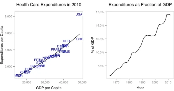
1.1 Facts about health care expenditures. Left: Health care expenditures and GDP per capita across OECD countries in 2010. Right: Evolution of U.S. health care expenditures as a fraction of GDP. Source: OECD System of Health Accounts (SHA); Authors’ analysis. Notes: Health care expenditures and GDP data are in 2010 dollars and adjusted for purchasing power parity. . . 7

1.2 Facts about health outcomes. Left: Life expectancy and health care ex-penditures per capita across OECD countries in 2010. Right: Infant mor-tality and health care expenditures per capita across OECD countries in 2010. Source: OECD System of Health Accounts (SHA); Authors’ analy-sis. Notes: Health care expenditures data are in 2010 dollars and adjusted for purchasing power parity. . . 7

1.3 Facts about health insurance allocation in the U.S. over time. Top left: Evolution of the share of uninsured. Top right: Evolution of the share with Medicare. Bottom left: Evolution of the share with Medicaid. Bot-tom right: Evolution of the share with private health insurance. Source: Medical Expenditure Panel Survey (MEPS); Authors’ analysis. . . 8

(15)

1.5 Survival probabilities by age, education level, and health status. Top left: Fixed low education level, varying age and health status. Top right: Fixed high education level, varying age and health status. Bottom left: Fixed bad health status, varying age and education level. Bottom right: Fixed

good health status, varying age and education level. . . 29

1.6 Observed and estimated Lorenz curves of assets. . . 30

1.7 Estimated medical expenditures by age and health status. Top left: Fixed bad health status, varying age and percentiles. Top right: Fixed good health status, varying age and percentiles. Bottom left: Fixed percentile 1st –60th , varying age and health status. Bottom right: Fixed percentile 61st –90th , varying age and health status. . . 33

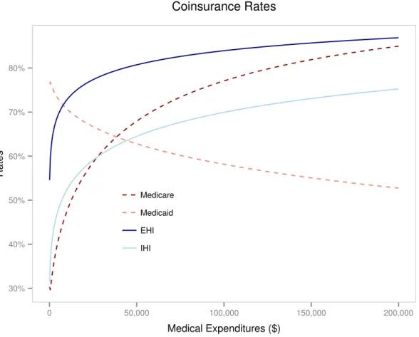
1.8 Coinsurance rates by type of coverage and medical expenditures. . . 36

1.9 Observed and simulated allocations of health insurance by age, education level, and health status. Notes: Data values are from the Medical Expen-diture Panel Survey (MEPS). Averages from 1996 to 2010. . . 41

1.10 Private health insurance premiums by age and health status. . . 42

1.11 Simulated allocations of health insurance by policy, age, low education level, and bad health status. . . 45

2.1 Survival Probabilities . . . 73

2.2 Observed and Estimated Lorenz Curves . . . 79

2.3 Variations in Inequality Measures. . . 82

(16)

List of Tables

1.1 Estimated Medical Expenditures in 2010 Dollars by Health Status and

Age Group . . . 32

1.2 Set of Average Lifetime Earnings . . . 34

1.3 Transitions of Productivity and EHI Oﬀer by Age Group 50–64 and Low Education . . . 38

1.4 Allocation of Health Insurance (%) . . . 41

1.5 Observed and Simulated Macroeconomic Variables . . . 42

1.6 Allocation of Health Insurance Before and After Policies (%) . . . 44

1.7 Variations in Government Budget Relative to Benchmark (%) . . . 47

1.8 Variations in Aggregate Variables and Prices Relative to Benchmark (%) . 48 1.9 Consumption Equivalent Variation of Newborns (%) . . . 51

1.10 Summary of Parameters . . . 56

2.1 Percentage of Net Worth Held by the Richest Groups (%) . . . 63

2.2 Average Net Worth Held by the Richest Groups (Aged 20-25) . . . 63

2.3 Percentage of Young Adults Aged between 20 and 25 (%) . . . 64

2.4 Set of Labor Times . . . 74

2.5 Labor Productivities, Transition Probabilities and Invariant Distribution . 75 2.6 Set of Average Lifetime Earnings . . . 76

2.7 Main Results . . . 80

2.8 Results Considering Fractions of Initial Assets . . . 81

2.9 Observed and Estimated Macroeconomic Variables . . . 83

(17)

(18)

Chapter 1

Health Care Reform vs. Cost

Reductions: A Quantitative

Assessment

1.1 Introduction

Health care costs in the U.S. are known to be high, especially when compared to other

OECD countries. According to the OECD System of Health Accounts (SHA), in 2010,

even controlling for income, population size, and cost of living, the U.S. spent 41.7%

more on health care than would be predicted by the OECD trend. This amounts to

$2,428 per year in excess for every American. At the same time, the share of uninsured

population in the U.S. is also high. According to the Medical Expenditure Panel Survey

(MEPS), the share of the population without health insurance was equal to 13.1% in

2010. These two facts combined generate a high risk of personal bankruptcy for millions

of Americans. According toHimmelstein et al.(2009), medical bills are the biggest cause of U.S. bankruptcies, and accounted for 62.1% of all bankruptcies in 2007. They also

concluded that the share of bankruptcies attributable to medical problems rose by 50%

between 2001 and 2007.

To address this issue, on March 23, 2010, President Barack Obama signed into law

(19)

increase health insurance coverage of the U.S. population. To achieve this goal, among

many features, the PPACA created a Health Insurance Marketplace where Americans

can purchase federally regulated and subsidized health insurance, expanded the Medicaid

program, and introduced a mandate where Americans are required to be covered by some

health insurance. However, this reform does not deal directly on reducing health care

costs, which seems to be a major issue of the U.S. health care system. Instead of

increas-ing public expenditures on health care and forcincreas-ing Americans to purchase insurance, the

reform could have focused on policies of health care costs reduction. For example,Cutler and Ly(2011) did an extensive review of international health care costs and highlighted four primary directions that could reduce U.S. health care costs.

In addition, the PPACA is not capturing the important link between high health

care costs and high share of uninsured population. After all, higher costs are reﬂected

in higher insurance premiums, leading to a high share of uninsured population. By this

reasoning, cost reductions could increase the share of covered population, and increasing

the share of insured without dealing with cost reductions may be a way of acting on the

consequences of the problem, and not on the cause. Besides, cost reductions can have a

potential positive welfare eﬀect by alleviating the budget of individuals.

Therefore, important questions with respect to public policy can be raised. What

would be better in terms of reducing the share of uninsured, the PPACA or policies of

realistic health care costs reduction? In addition, which would be better in terms of

the welfare of individuals? What is the long run impact of these policies on government

budget?

To answer these questions, we built a life cycle general equilibrium model with

hetero-geneous agents to compare the eﬀects of the PPACA and of health care costs reduction

policies on health insurance coverage, government budget, and welfare of individuals.

This economy consists of a large number of heterogeneous agents, competitive

produc-tion and health insurance sectors, and a government. Agents diﬀer by age, educaproduc-tion

level, health status, asset holdings, medical expenditures, labor productivity, average

lifetime earnings, employer-sponsored health insurance (EHI) oﬀer, and health insurance

coverage. There are uncertainties regarding the age of death, health status, medical

(20)

time, next period’s asset holdings, and next period’s health insurance coverage. Medical

expenditures are costly relative to consumption. Five types of health insurance

cov-erage are available: Medicare, Medicaid, employer-sponsored health insurance (EHI),

individual health insurance (IHI), and no insurance. Premiums of private insurances are

determined endogenously. Retirement is exogenous and the income tax is progressive and

follows the current law for tax beneﬁts on health insurance and medical expenditures.

The model is calibrated to the U.S. economy before the introduction of the PPACA,

and is able to reproduce very closely the allocation of health insurance and some key

macroeconomic variables. In particular, the model reproduces the high share of uninsured

population and the fact that most of the population purchases health insurance through

employer. We then simulated the model considering four changes introduced by the

PPACA: the premium tax credits, the individual mandate, the Medicaid expansion, and

the increase in income threshold for claiming deduction of medical expenses in income

tax. These changes were simulated individually, to capture the net eﬀect of each one,

and then together, to capture the eﬀect of the reform as a whole.

Cost reductions were implemented exogenously by reducing the relative price of

med-ical expenses to consumption.1

We performed two experiments. First, to carry out a

realistic and politically feasible experiment, we implemented the estimated cost

reduc-tions calculated byLiu et al.(2014), which is a Rand Corporation project that identiﬁed fourteen ideas for relatively focused changes that would generate health care cost savings

at the national level. Second, as a counterfactual benchmark, we applied to the model

the same percentage reduction in per capita health care expenditures required to bring

the U.S. to the OECD trend in 2010. We call these experiments the “Rand Proposal”

and “OECD Trend”, respectively.2

We found that all experiments were able to reduce uninsured population, with the

PPACA being more eﬀective than both cost reduction experiments. Except for the

in-crease in income threshold for claiming deduction of medical expenses, all other PPACA

1

From 2000 to 2011,Moses et al.(2013) found that price (especially of hospital charges, professional services, drugs and devices, and administrative costs), but not demand for services or aging of the population, accounted for 91% of total health care cost increase.

2

(21)

changes were individually more eﬀective than cost reductions, with the Medicaid

expan-sion being the most eﬀective. The PPACA as a whole reduced the uninsured population

by 70.7%, while the Rand Proposal and the OECD Trend reduced by 2.7% and 12.3%,

respectively.

The impact on government budget walked in opposite directions. The PPACA

in-creased public deﬁcit, mainly due to the Medicaid expansion. To rebalance its budget,

the government increased the consumption tax rate by 10.5%. In contrast, health care

cost reductions alleviated the ﬁscal burden of public insurance, reducing public deﬁcit.

The reduction in the consumption tax rate caused by the Rand Proposal and OECD

Trend were 1.3% and 40.4%, respectively.

Regarding welfare eﬀects, we found that the PPACA as whole and cost reductions

were welfare improving. The OECD Trend was the most successful in improving welfare,

demonstrating the importance of reducing health care costs. Except for the Medicaid

Expansion, the Rand Proposal was better than all other PPACA changes, showing that

feasible cost reductions could be a good alternative. The individual mandate and the

increase in income threshold for claiming deduction of medical expenses in income tax

generated negative welfare eﬀects. However, the large positive eﬀects of the Medicaid

expansion made the PPACA as a whole to be better than the Rand Proposal.

Our work relates to the literature that uses quantitative models to perform ex ante

policy evaluations regarding health care issues. Jeske and Kitao (2009) study tax sub-sidies for group health insurance, Attanasio et al. (2010) analyze alternative funding schemes for Medicare,Feng(2010) and Hsu and Lee (2013) investigate public provision for universal health insurance,Hansen et al.(2014) evaluate the consequences of expand-ing Medicare program, Janicki (2014) access the role of asset testing in public health insurance reform, and Pashchenko and Porapakkarm (2015) evaluate the importance of reclassiﬁcation risk in the health insurance market.

The work most closely related to ours isPashchenko and Porapakkarm(2013), which use a quantitative model to evaluate which component of the PPACA contributes more

to the welfare outcome of the reform. Our key contribution to the literature is that we

compare the eﬀects of the PPACA with other alternatives that deal directly with health

(22)

Besides, we also extended their model in some dimensions. First, we explicitly

con-sider health status as a characteristic of individuals, allowing us to condition preferences,

survival probabilities, and medical expenditures on health status. Second, we allow

med-ical expenditures to be costly relative to consumption, which is key for our cost reduction

experiments. Third, we allow hours worked to vary both in the extensive and intensive

margins, generating more heterogeneity in labor income. Fourth, our Social Security

sys-tem is closer to the rules of the Social Security Administration (SSA), with beneﬁts being

a function of average lifetime earnings of each individual. Fifth, our progressive income

tax schedule exactly follows the rules of the Internal Revenue Service (IRS). The last

three features are important for building an enabling environment for the determination

of labor income, which in turn has a major role in the rules imposed by the PPACA, as

well as being key for Medicaid eligibility.

Our work also relates to the literature that uses quantitative models with features of

health status, medical expenditures, and/or health insurance. Palumbo (1999) and De Nardi et al.(2010) study the effects of uncertain medical expenses on precautionary saving of the elderly,French(2005) analyze the effects of health on labor supply and retirement behavior, French and Jones (2011) investigate the effects of employer-sponsored health insurance and Medicare on retirement behavior,Ferreira and dos Santos(2013) quantifies the effects of Medicare on the expansion in retirement,Hsu(2013) evaluate the relation between health insurance and precautionary saving, Zhao (2014) access the relation of Social Security and the rise in aggregate health spending,Kopecky and Koreshkova(2014) evaluate the impact of nursing home expenses on savings of the elderly, and Zhao(2015) analyze the impact of health shocks on the demand for health insurance and annuities,

along with precautionary saving.

The remainder of the article is organized as follows. In the next section, we present

some stylized facts about health care costs and health insurance allocation. In Section

1.3, we describe our model economy. In Section1.4, we present the changes introduced by the PPACA and how they were implemented in the model. In Section1.5, we explain the cost reduction experiments. In Section 1.6, we present the model parameterization. In Section1.7, we report the performance of the model in replicating the data. In Section

(23)

concluding comments.

1.2 Stylized Facts

Countries with higher incomes tend to spend more on health care. However, even taking

this relationship into account, the United States spends far more on health care than

might be predicted. In the left panel of Figure 1.1, we compare total health care expen-ditures between OECD countries, showing that the amount spent by the U.S. is far more

than would be expected even adjusting for population size and relative wealth diﬀerences.

In 2010, the U.S. spent 41.7% more than would be predicted by the OECD trend, which

amounts to $2,428 per year in excess for every American.3 _{The right panel of Figure}_1.1

presents the evolution of U.S. health care expenditures as a fraction of GDP, showing

that it has increased substantially, going from 5.68% in 1965 to 17% in 2009, a growth

of 200%.

Someone might argue that this excessive spending on health care can be justiﬁed by

a superior health status of Americans. However, this does not seem to be the case. In

Figure1.2, we analyze among the OECD countries two popular measures of a population’s health: life expectancy and infant mortality. For both measures, in 2010, the U.S.

result is worse than what would be expected after adjusting for population size and total

health care expenditures. Life expectancy in the U.S. is below the ﬁrst quartile of the

distribution of countries, and Americans live about 5 years less than would be predicted

by the OECD trend. Infant mortality in the U.S. is above the third quartile of the

distribution of countries, and exhibit about 3.4 more deaths per 1,000 live births than

would be predicted by the OECD trend.

In a scenario where medical expenditures are excessive, health insurance becomes

essential. In Figure1.3, we present the evolution of health insurance allocation in the U.S. in a pre-PPACA period. From 1999 to 2010, there was a reallocation of the population

with private insurance to public insurance or no insurance. The share of uninsured

increased 2.2 percentage points, reaching 13.1% by the end of the period. The share

3

(24)

AUS AUT BELCAN CHL CZE DNK EST FIN FRADEU GRC HUN ISL IRL ISR ITAJPN KOR MEX NLD NZL POL PRT SVK SVN ESP SWE CHE TUR GBR USA 2,000 4,000 6,000 8,000

20,000 30,000 40,000 50,000

GDP per Capita

Expenditures per Capita

Health Care Expenditures in 2010

7.5% 10.0% 12.5% 15.0% 17.5%

1970 1980 1990 2000 2010

Year

% of GDP

Expenditures as Fraction of GDP

Figure 1.1: Facts about health care expenditures. Left: Health care expenditures and GDP per capita across OECD countries in 2010. Right: Evolution of U.S. health care expenditures as a fraction of GDP. Source: OECD System of Health Accounts (SHA); Authors’ analysis. Notes: Health care expenditures and GDP data are in 2010 dollars and adjusted for purchasing power parity. AUS AUT BEL CAN CHL CZE DNK EST FIN FRA DEU GRC HUN ISL IRL ISR ITA JPN KOR MEX NLD NZL POL PRT SVK SVN ESP SWE CHE TUR GBR USA 74 76 78 80 82 84

2,000 4,000 6,000 8,000

HC Expenditures per Capita

Age

Life Expectancy in 2010

AUSAUT_BEL CAN CHL CZE DNK EST FIN FRA_DEU GRC HUN ISL IRL ISR ITA JPN KOR MEX NLD NZL POL PRT SVK

SVNESPSWE CHE TUR GBR USA 0 5 10 15

2,000 4,000 6,000 8,000

HC Expenditures per Capita

Deaths per 1,000 Liv

e Bir

ths

Infant Mortality in 2010

Figure 1.2: Facts about health outcomes. Left: Life expectancy and health care expenditures per capita across OECD countries in 2010. Right: Infant mortality and health care expenditures per capita across OECD countries in 2010. Source: OECD System of Health Accounts (SHA); Authors’ analysis. Notes: Health care expenditures data are in 2010 dollars and adjusted for purchasing power parity.

with public insurance also rose, with the Medicare and Medicaid increasing 1.0 and 5.6

percentage points, reaching 12.8% and 15.8% in 2010, respectively. On the other hand,

the share with private health insurance decreased 8.8 percentage points, reaching 58.3%

(25)

10% 11% 12% 13% 14%

1996 1998 2000 2002 2004 2006 2008 2010

Year

Share of P

opulation

Uninsured

10% 11% 12% 13% 14%

1996 1998 2000 2002 2004 2006 2008 2010

Year

Share of P

opulation

Medicare

10% 12% 14% 16%

1996 1998 2000 2002 2004 2006 2008 2010

Year

Share of P

opulation

Medicaid

55% 60% 65% 70%

1996 1998 2000 2002 2004 2006 2008 2010

Year

Share of P

opulation

Private

Figure 1.3: Facts about health insurance allocation in the U.S. over time. Top left: Evolution of the share of uninsured. Top right: Evolution of the share with Medicare. Bottom left: Evolution of the share with Medicaid. Bottom right: Evolution of the share with private health insurance. Source: Medical Expenditure Panel Survey (MEPS); Authors’ analysis.

costs. Higher costs are reﬂected in private insurance premiums, making private insurance

unaﬀordable, forcing people to rely on public insurance or to become uninsured.

1.3 Model Economy

We built a life cycle general equilibrium model in the tradition of İmrohoroğlu et al.

(1995),Huggett(1996),İmrohoroğlu et al.(1999), andHuggett and Ventura(1999). We extended these models to consider features of health status, medical expenditures, and

(26)

agents, a competitive production sector, a competitive health insurance sector, and a

government with a commitment technology. Time is discrete and one model period

is a year. All shocks are independent among agents and, as a consequence, there is no

uncertainty over the aggregate variables even though there is uncertainty at the individual

level.

1.3.1 Education Level

The economy is populated by a large number of heterogeneous agents with age j ∈

{1,2, . . . , J}. Agents enter the economy with education level e ∈ {eL_{, e}H_}_{, where} _eL

means low education and eH _{means high education. The education level is exogenously}

given and retained throughout life. The probability of agents entering the economy with

education leveleis given by Λ(e).

1.3.2 Health Status

Agents face exogenous uncertainty about their health status h ∈ {hB_{, h}G_}_{, where} _hB

means bad health and hG _{means good health. The health status is assumed to evolve}

over time according to a ﬁrst-order Markov process, where the transition probabilities

depend on age and education level. Conditional on being at age j, with education level

e, and current health statush, the probability of having next period’s health statush′ is given byΦj,e(h, h′).

1.3.3 Demography

The population grows exogenously at a constant rate η. Agents also face exogenous un-certainty regarding the age of death. Conditional on being alive at agej, with education levele, and current health statush, the probability of surviving to age(j+ 1)is given by

Πj,e,h. Since all agents enter alive in the economy with age j = 1, we must assume that Π0,e,h = 1 for all (e, h). Besides, agents die with certainty at the end of age J, which

means thatΠJ,e,h= 0for all(e, h). The share of agents of type(j, e, h) is given byµj,e,h

and can be recursively deﬁned as

µj+1,e,h′ =

(27)

1.3.4 Asset Market

Agents can acquire a one-period riskless asset in each period of life. The total resources

used to acquire the assets are exogenously divided between the productive sector in the

form of capital and the government in the form of debt. Current asset holdings is denoted

bya∈ A, where the set of assetsAis ﬁnite. Agents enter the economy with a endowment of assets drawn from the distribution Ω(a). The riskless rate of return on asset holdings is denoted by r. Agents are not allowed to incur debt at any age, so that the amount of assets carried over from age j to (j+ 1) is such thata′ _≥₀_{, where}_a′ _{is next period’s} asset holdings. For simplicity, we assume that all assets left by the deceased are collected

by the government and distributed to the live agents as a lump-sum bequest transferB.

1.3.5 Preferences

In each period of life, agents are endowed withℓunits of time, which can be split among labor and leisure. The choice of labor time is given byl∈0, lP_{, l}F _{, where}_lP _{is the time}

needed for a part-time job,lF _{is the time needed for a full-time job, and}₀_{< l}P _{< l}F _{< ℓ}_.

Agents enjoy utility over consumption, leisure, and accidental bequests, and maximize

the discounted expected utility throughout life. The intertemporal discount factor is

given by β. We model the eﬀect of health status on utility as a ﬁxed time cost.4

In

addition, there is a cost of work treated as a loss of leisure.

Our utility speciﬁcation is based on French (2005). The period utility function over consumption, leisure, and health status is given by

u(c, l, h) =

cγ_ℓ₋_l₋_φ

11{l >0}−φ21{h=hB_}

1−γ1−σ

1−σ ,

wherecis the consumption,γ is the share of consumption in utility,σ is the risk aversion parameter, φ1 is the time cost of work, φ2 is the time cost associated with bad health status, and1{·}is an indicator function that maps to one if its argument is true. The term

in parentheses represents leisure time. The “warm-glow” utility from leaving accidental

4

(28)

bequests is given by

uB(a′) =ψ1(ψ2+a

′₎γ(1−σ)

1−σ ,

whereψ1 represents the weight on the utility from bequeathing andψ2 aﬀects its curva-ture.

1.3.6 Medical Expenditures

Agents incur medical expenditures during each period of life, which are treated as

nec-essary consumption that generates no utility but must be paid. Such expenditures do

not include expenses with public or private health insurance. The current medical

ex-penditures of an agent are denoted by m∈ Mj,h, where the set of medical expenditures

Mj,h is ﬁnite and depends on age and current health status. Medical expenditures are

costly relative to consumption. The relative price of medical expenditures to

consump-tion is denoted byπ, which implies that the value of expenditures incurred by agents is expressed asπm. Agents face exogenous uncertainty about next period’s medical expen-ditures, which are drawn from the distribution Ψj,h(·) that depends on age and health

status. Therefore, conditional on being at age j, with education level e, and current health status h, the probability of incurring in next period’s medical expenditures m′, with next period’s health statush′, is given byΦj,e(h, h′)Ψj+1,h′(m′).

1.3.7 Labor Productivity

In each period of life, agents receive an idiosyncratic labor productivity shock that is

revealed at the beginning of the period. We denote this shock by z ∈ Z, where the set of labor productivities Z is ﬁnite. This productivity shock follows a ﬁrst-order Markov

process that evolves jointly with the oﬀer of an employer-sponsored health insurance

(29)

1.3.8 Social Security

Once agents reach the retirement age R, they automatically stop working and start receiving Social Security beneﬁt. This beneﬁt depends on the average lifetime earnings

of an agent, which is calculated by taking into account individual earnings up to age

(R−1).5

We denote the average lifetime earnings by x ∈ X, where the set of average lifetime earnings X is ﬁnite. It can be recursively deﬁned as

x′ =

      

x(j−1) + miny, ySS

j if j < R,

x if j≥R,

whereySS is theSocial Security Wage Base(SSWB), which is the maximum earned gross income at which the Social Security tax applies.

Let b(x) be the Social Security beneﬁt function, which corresponds to the Primary

Insurance Amount(PIA).6 _{This beneﬁt is calculated as a piecewise linear function, which}

in accordance with the rules of the U.S. Social Security system is given by

b(x) =

              

θ1x if x≤x1,

θ1x1+θ2(x−x1) if x1 < x≤x2,

θ1x1+θ2(x2−x1) +θ3(x−x2) if x2 < x≤ySS,

where{x1, x2}are the bend points of the function and the parameters{θ1, θ2, θ3}satisfy

0≤θ3< θ2 < θ1.

1.3.9 Health Insurance

There are four types of health insurance coverage in the economy: Medicare, Medicaid,

employer-sponsored health insurance (EHI), and individual health insurance (IHI). The

ﬁrst two are public, provided by the government, and the last two are private, provided

by health insurance ﬁrms. There is also the possibility to have no insurance coverage.

5

According to the Social Security legislation, the average lifetime earnings should be calculated by taking into account the 35 highest individual earnings up to theEarliest Retirement Age. For simplicity, we consider the whole history of earnings, since it is hard to identify the 35 highest earnings when solving the model.

6

(30)

Leti∈i0, iM C_{, i}M A_{, i}E_{, i}I _{be the type of health insurance that an agent has, where}_i0 means no coverage,iM C means coverage by Medicare, iM A means coverage by Medicaid,

iE _{means coverage by employer-sponsored health insurance, and} _iI _{means coverage by}

individual health insurance.

A health insurance is a one-period contract where the insured commits to pay a

pre-mium today and the insurer commits to cover a fraction of realized medical expenditures

in the next period. Thus, the type of insurance coverage that an agent has today was

contracted the period before, and the premium that an agent pays today is for the next

period’s coverage. The coinsurance rate of an agent’s coverage is given byq(i, m), which depends on the current health insurance type i and the realized medical expenditures

m. The premium paid by an agent is given by p(i′, j, h), which depends on the choice of next period’s health insurance type i′_{, the age} _j_{, and the current health status} _h_. Naturally, we assume that q i0_{, m} _{= 0} _{for all} _m _and _{p i}0_{, j, h} _{= 0}_{for all} ₍_{j, h}₎_{. For} ease of notation, we denote the medical expenditures actually paid by

e

m= [1−q(i, m)]πm.

The government provides health insurance for the elderly through Medicare. Once

agents reach the ageR, they are automatically enrolled in this program. This means that agents aged (R−1)and older cannot choose any other type of health insurance. This program charges a ﬁxed premium for all eligible agents, which means thatp iM C_{, j, h}₌

pM C _{for all} ₍_{j, h}₎_{. The government incurs in administrative costs} _ϕ _{per unit of medical}

expenditures covered by the program. We denote the eligibility criteria for Medicare as

an indicator function given by

1M C=

      

1 if j≥R−1,

0 if j < R−1.

Agents can obtain their health insurance from Medicaid for free, which means that

p iM A_{, j, h}_{= 0}_{for all}₍_{j, h}₎_{. There are two pathways to qualify for this program. First,}

(31)

yM A_{. Second, agents can become eligible through the Medically Needy program. This}

happens if the labor income plus asset income, minus medical expenditures actually paid,

is less than or equal the thresholdyM N_{, and if the assets are less than or equal the limit}

aM N_{. Thus, the eligibility criteria for Medicaid can be represented by}

1M A =

              

1 if y+ra≤yM A_,

1 if y+ra−me ≤yM N _and _a_≤_aM N_,

0 otherwise.

Agents may receive an exogenous oﬀer of an employer-sponsored health insurance

(EHI), which can be accepted only if the agent chooses to work. We denote the status

of this offer by ι ∈ {0,1}, where ι = 0 means that the agent did not receive the offer andι= 1 means that the agent received the offer. We assume thatιfollows a first-order Markov process that evolves jointly with the labor productivity shock z. The transition probabilities of this process depend on age and education level. Conditional on being at

age j, with education level e, and current productivity-oﬀer pair (z, ι), the probability of having next period’s productivity-oﬀer pair(z′, ι′) is given by Γj,e(z, ι, z′, ι′). We can represent the criteria if an agent is eligible to choose an EHI coverage by

1E =

      

1 if ι= 1 and l >0,

0 otherwise.

As required by law, screening is not allowed when determining the EHI premium,

which means that all participants of the employer-based poll are charged the same ﬁxed

premium. Besides, an employer oﬀering EHI must pay a fractionωof the premium. Thus, the premium that agents pay for this type of health insurance is given by p iE, j, h=

(1−ω)pE for all(j, h). Every agent has access to individual health insurance (IHI) under any circumstances. Screening is allowed for this type of health insurance, which means

that the premium really depends on age and health status. Thus, the premium that

agents pay for the IHI coverage is given byp iI_{, j, h}₌_pI₍_{j, h}₎_.

(32)

the options that an agent is eligible to choose. Since Medicaid is free, we assume that

a Medicaid-eligible agent cannot stay uninsured. Therefore, the set of choices for next

period’s health insurance must satisfy

i′ ∈                               

i0_{, i}I _if

1M C = 0 and 1M A= 0 and 1E = 0,

i0, iE_{, i}I _if ₁M C _{= 0} _and ₁M A_{= 0} _and ₁E _{= 1}_,

iM A_{, i}I _if

1M C = 0 and 1M A= 1 and 1E = 0,

iM A_{, i}E_{, i}I _if ₁M C _{= 0} _and ₁M A_{= 1} _and ₁E _{= 1}_,

iM C _if

1M C = 1.

(1.1)

1.3.10 Taxation

All agents pay income taxτY _yT_{, which is a progressive function of taxable income}_yT_.

The taxable income is based on labor income and asset income. According to the current

law for tax beneﬁts, the amount of the EHI premium paid by agents is tax deductible in

calculating income taxes. Besides, agents can also deduct medical expenditures actually

paid that exceed a fractionξ of the labor income plus asset income.7

Therefore, taxable

income can be formalized by

yT = maxny+ra−(1−ω)pE1{i′₌_iE_}−max{me −ξ(y+ra),0},0 o

.

7

(33)

For the progressive income tax function, we follow the 2010 Internal Revenue Service

(IRS) rules and assume that

τY yT=

                                              

τ1yT if yT ≤y1,

τ1y1+τ2 yT −y1

if y1 < yT ≤y2,

τ1y1+τ2(y2−y1) +τ3 yT −y2 if y2 < yT ≤y3,

τ1y1+ 3 X

n=2

τn(yn−yn−1) +τ4 yT −y3

if y3 < yT ≤y4,

τ1y1+ 4 X

n=2

if y4 < yT ≤y5,

τ1y1+ 5 X

n=2

if y5 < yT,

where {τ1, τ2, τ3, τ4, τ5, τ6} are the marginal income tax rates and {y1, y2, y3, y4, y5} are the income brackets.8

Agents also pay a consumption tax τC_{, which is proportional and levied directly on}

consumption. Workers must pay a Social Security tax τSS_{, which is proportional and}

levied on the minimum between labor income and the Social Security wage base. These

agents also have to pay a Medicare tax τM C_{, which is proportional and levied on labor}

income. The EHI premium is also tax deductible in calculating taxes from Social Security

and Medicare. We can formalize the Social Security and Medicare taxes, respectively, by

TSS =τSSminnmaxny−(1−ω)pE1{i′₌_iE_},0 o

, ySSo

and

TM C=τM Cmaxny−(1−ω)pE1{i′₌_iE_},0 o

.

For ease of notation, we deﬁne the total taxes paid by agents, excluding the consumption

tax, by

T =τY yT+TSS+TM C.

8

To the best of our knowledge, every article in the quantitative macroeconomic literature that con-siders a progressive income tax function uses the functional form estimated by Gouveia and Strauss

(34)

1.3.11 Social Insurance

The Social Insurance is a means-tested program that guarantees a minimum level of

consumption cto every agent by supplementing income with a lump-sum transfer TSI_.9

We follow Hubbard et al. (1995) and assume that this transfer occurs if c is greater than the total income minus the necessary expenditures. The total income is deﬁned as

the sum of labor income (or Social Security beneﬁt), total assets, and bequest transfer.

The necessary expenditures are deﬁned as the sum of taxes and medical expenditures

actually paid. If the agent is insured by Medicare, we consider the Medicare premium as

a necessary expenditure. Therefore, we can formalize the Social Insurance transfer by

TSI =

                      

max 1 +τC_c₊_T ₊

e

m−y−(1 +r)a−B, 0 if j≤R−2,

max 1 +τC_c₊_T ₊_m_e ₊_pM C₋_y₋_{(1 +}_r₎_a₋_B,₀ _if _j₌_R₋₁_,

max 1 +τC_c₊_T ₊

e

m+pM C₋_b₍_x₎₋_{(1 +}_r₎_a₋_B,₀ _if _R_≤_{j < J,}

max 1 +τCc+T +me −b(x)−(1 +r)a−B,0 if j=J.

1.3.12 Production Sector

We assume that there are two representative ﬁrms which act competitively and produce

a single consumption good. Both ﬁrms maximize proﬁts renting capital and labor from

agents, and pay an interest raterand a wage ratewfor these factors, respectively. Their production functions are the same and take the form of a Cobb-Douglas speciﬁcation,

which is given by F(K, L) = AKα_L1−α_{, where} _K _and _L _{are the aggregate capital and}

labor inputs,Ais the total factor productivity, andαis the share of capital in the output. Capital is assumed to depreciate at a rateδ each period.

The difference between the two firms lies in the fact that one offers EHI to its workers

and the other not. The ﬁrm that oﬀers the insurance must pay a fraction of the premiums

for the agents who have accepted the oﬀer. This cost is passed on to all its employees

through a wage rate reduction. In specifying this reduction, we follow Jeske and Kitao

(2009) and assume that this ﬁrm subtract the amount χ from the wage rate of all its 9

(35)

workers. This amount is just enough to cover the total premium cost for the ﬁrm.

Indexing by0 the firm that does not offer EHI and by1 the firm that offers EHI, we

can write the problems of the two ﬁrms as

max K0,L0

F(K0, L0)−(r0+δ)K0−w0L0

and

max K1,L1

F(K1, L1)−(r1+δ)K1−(w1+χ)L1.

The ﬁrst order conditions imply that the factor prices paid by both ﬁrms are given by

r0 =αA

K0

L0 α−1

−δ,

w0 = (1−α)A

K0

L0 α

,

r1 =αA

K1

L1 α−1

−δ,

w1 = (1−α)A

K1

L1 α

−χ.

Assuming that capital is freely allocated between the two ﬁrms, by no arbitrage we have

thatr0 =r1 ≡r. This implies that the capital-labor ratio of both ﬁrms are equal, that is, K0/L0 =K1/L1. Therefore, we conclude that w1 =w0−χ≡w−χ. Thus, from the agents’ point of view, we can summarize the wage rate received by a worker as being

e w=       

w if ι= 0,

w−χ if ι= 1.

1.3.13 Health Insurance Sector

We assume that there is a representative and competitive health insurance ﬁrm operating

each type of private health insurance contract. In our model, there is only one type of

EHI contract and an IHI contract for each pair (j, h). The premiums collected by the ﬁrms are invested in the asset market. These ﬁrms can observe all the variables that

(36)

per unit of medical expenditures covered. There is also a ﬁxed cost κ for providing IHI.

This ﬁxed cost captures the diﬀerence in overhead costs between IHI and EHI.10

1.3.14 Government

The government manages all the social programs: Social Security, Medicare, Medicaid,

and Social Insurance. Its revenues are provided from taxes, Medicare premiums, and

issuance of one-period riskless debtD, which by no arbitrage must carry the same return in equilibrium as claims to capital. These revenues ﬁnance the Social Security beneﬁts,

the Medicare and Medicaid coverage, the Social Insurance transfers, the government

expenditures G, and the servicing and repayment of the debt.

1.3.15 Agents’ Problem

There are two groups of heterogeneous agents, workers and retirees. Workers are those

aged(R−1)and younger, while retirees are those agedRand older. LetSW _and_SR_be

the state spaces of workers and retirees, respectively. The state vector of a worker is given

by sW = (j, e, h, a, m, z, x, ι, i)∈ SW, and its value function is given by VW :SW → R.

Similarly, the state vector of a retiree is given by sR = (j, e, h, a, m, x) ∈ SR, and its

value function is given byVR_:_SR_→_R_{. The agents’ problem must be solved separately}

for speciﬁc age groups. Therefore, we describe the problem by dividing it between the

age groups.

For j ∈ {1, . . . , R−2}, agents are workers in the current period and will remain workers in the next period. They choose consumption, labor supply, next period’s asset

holdings, and next period’s health insurance coverage. Their problem can be recursively

deﬁned as

VW(sW) = max

(c,l,a′_,i′₎

u(c, l, h) +β

Πj,e,hEVW s′W

+ (1−Πj,e,h)uB(a′)

10

(37)

subject to

1 +τCc+a′+m_e +p i′, j, h+T =y+ (1 +r)a+TSI+B,

c≥0, l∈0, lP, lF , a′ ≥0,

with i′ _{satisfying equation (}_1.1_{). For} _j _{= (}_R₋₁₎_{, there are two diﬀerences in relation} to the above problem. First, because these agents will be retirees in the next period,

they take into account the expected value function of retirees in the next period rather

than the expected value function of workers. Second, as they will automatically have

Medicare in the next period, they pay the ﬁxed Medicare premium and no longer choose

next period’s health insurance coverage.

For j ∈ {R, . . . , J−1}, agents are retirees in the current period and will remain retirees in the next period, no longer choosing labor supply. They choose consumption

and next period’s asset holdings, and receive Social Security beneﬁt in the current period.

Their problem can be recursively deﬁned as

VR(sR) = max

(c,a′₎

u(c,0, h) +β

Πj,e,hEVR s′_R+ (1−Πj,e,h)uB(a′)

subject to

1 +τCc+a′+me +pM C+T =b(x) + (1 +r)a+TSI+B,

c≥0, a′≥0.

For j = J, there are two diﬀerences in relation to the above problem. First, because these agents will be dead next period, they no longer take into account the expected

value function of retirees in the next period, considering only the utility from leaving

accidental bequests. Second, because they will no longer use the Medicare coverage next

period, they do not pay the ﬁxed Medicare premium.

(38)

1.4 Health Care Reform

In this section we present the PPACA policy changes and show how they were

imple-mented in the model. We ﬁrst present and discuss the concept of aﬀordable health

in-surance created by the reform. Then we detail the four policies that were evaluated: the

premium tax credits, the individual mandate, the Medicaid expansion, and the increase

in income threshold for claiming deduction of medical expenses in income tax.

1.4.1 Affordable Health Insurance

An important concept created by the reform is aﬀordable health insurance. This concept

is important to determine who will receive premium tax credits and who will be exempt

from paying penalties for being uninsured. If an agent is not eligible to choose an EHI

coverage, then the IHI contract will be considered aﬀordable if its premium costs less

than or equal a fractiondI _{of the agent’s labor income plus asset income. On the other}

hand, if an agent is eligible to choose an EHI coverage, then the EHI contract will be

considered aﬀordable if the part of the premium that should be paid by the agent costs

less than or equal a fraction dE _{of the agent’s labor income plus asset income. The}

aﬀordable health insurance criteria can be formalized as

1A=

              

1 if 1E = 0 and pI₍_{j, h}₎_≤_dI₍_y₊_ra₎_,

1 if 1E = 1 and (1−ω)pE _≤_dE₍_y₊_ra₎_,

0 otherwise.

1.4.2 Premium Tax Credits

After the reform, agents who can not aﬀord health insurance are eligible to receive a tax

credit to buy health insurance in the individual market. The tax credit structure ensures

that agents within a certain income category do not spend more than a certain fraction

of their income on health insurance. The income categories are based on a range of the

(39)

lower the premium will cost. The premium tax credit can be formalized as

TP =

                                              

pI(j, h)−ε1(y+ra) if 1A= 0 and i′ =iI and g1f ≤(y+ra)< g2f,

pI₍_{j, h}₎₋_ε

2(y+ra) if 1A= 0 and i′ =iI and g2f ≤(y+ra)< g3f,

pI(j, h)−ε3(y+ra) if 1A= 0 and i′ =iI and g3f ≤(y+ra)< g4f,

pI₍_{j, h}₎₋_ε

0 otherwise,

where {ε1, . . . , ε6} are the fractions of income spent on insurance and {g1, . . . , g7} are the fractions of the FPL that determine the income categories. In order to reﬂect the

premium tax credit in the model, we need to add the credit on the right hand side of

the agents’ budget constraints and add the aggregate credit on the left hand side of the

government budget.

1.4.3 Individual Mandate

The reform states that uninsured agents must pay a penalty to the government unless

they are qualiﬁed for a exemption. The penalty is equal to the maximum between the

valueυ and a fractionν of the taxable income. In addition, the maximum value of the penalty is equal to ρ. Uninsured individuals are exempt from the penalty if they cannot aﬀord a health insurance coverage. The penalty can be formalized as

TM =

      

minmaxυ, νyT _{, ρ} _if ₁A_{= 1} _and _i′ ₌_i0_,

0 otherwise.

In order to reﬂect the individual mandate in the model, we need to add the penalty on

the left hand side of the agents’ budget constraints and add the aggregate penalty on the

(40)

1.4.4 Medicaid Expansion

The reform expands the Medicaid eligibility to all agents younger thanRand with income below a fractionζ of the FPL. This new income threshold is higher than the current one, meaning that more individuals can have access to Medicaid after the expansion. There are

no changes in the Medically Needy Program. In order to reﬂect the Medicaid expansion

in the model, we just need to change the value of the parameter yM A _to _ζf_.

1.4.5 Deductible Medical Expenditures

The reform increases the income threshold for claiming the deduction for medical

ex-penditures. This will make it much more diﬃcult to qualify for deductions. Besides,

increasing the threshold also means that the deductions for medical expenditures will be

reduced. In order to reﬂect this change in the model, we just need to change the value

of the parameterξ to the new threshold.

1.5 Cost Reductions

In this section we present the two cost reduction experiments evaluated: the “Rand

Proposal” and the “OECD Trend”. The Rand Proposal, detailed inLiu et al. (2014), is a Rand Corporation project that identiﬁed fourteen ideas for relatively focused changes

that would generate health care cost savings.11 _{As argued by the authors, these ideas}

are quite feasible to implement and are only moderately politically sensitive.12 _Savings

were estimated at the national level in 2012 dollars, and considering the national health

expenditures of 2012 reported by the Centers for Medicare & Medicaid Services (CMS),

this amounts to an annual cost reduction of 0.64%. The proposal was reﬂected in the

model by applying this reduction to the relative price of medical expendituresπ. In the OECD Trend experiment, we applied to the model the same percentage

re-duction in per capita health care expenditures required to bring the U.S. to the OECD

trend in 2010, as shown in the left panel of Figure 1.1. The trend was calculated as a power ﬁt with the GDP per capita as the independent variable and the health care

11

See Tables 1 and 2 ofLiu et al.(2014) for the description and savings estimate of each idea, respec-tively.

12

(41)

expenditures per capita as the dependent variable. Data is from the OECD System of

Health Accounts (SHA), and all values are in 2010 dollars and adjusted for purchasing

power parity. Given the U.S. GDP per capita, the U.S. health care expenditures per

capita predicted by the trend should be 29.5% lower. We applied this reduction to the

relative price of medical expenditures π. We do not know which public policies would be able to generate such a reduction, and we believe that policies capable of that must

be diﬃcult to be approved and implemented. However, this reduction makes the U.S.

comparable in terms of per capita health care spending with the OECD countries, and

serves as a benchmark.

1.6 Model Parametrization

We parameterized the model using several diﬀerent data sources. Three sources of

mi-cro data were used: the Medical Expenditure Panel Survey (MEPS),13

the Health and

Retirement Study (HRS),14

and the Survey of Consumer Finances (SCF).15

Our main

source of macro data is the Council of Economic Advisers(2013). Other sources of data were used and will be appropriately cited.

1.6.1 Education Level

The high education level eH _{corresponds to at least a college degree, and the low}

educa-tion leveleLcorresponds to at most an incomplete college. To calculate the probabilities of education level, we used the data from Barro and Lee (2012).16

We used data for

the years 1990, 1995, 2000, 2005, and 2010, and considered the age groups of individuals

aged 20 and over. For each year-age pair, this data set provides the estimated population

and the share of population that completed the tertiary education. All data were pooled

in order to calculate the average across years and age groups. Using the estimated

popu-lation as weights, we calculated the weighted average of the share of the popupopu-lation that

completed the tertiary education. We assigned this value to Λ eH_{. The ﬁnal values}

obtained areΛ eH_{= 28}_._28% _and _Λ _eL_{= 71}_._72%_.

13

Seehttp://meps.ahrq.gov/mepsweb/. 14

Seehttp://hrsonline.isr.umich.edu/. 15

Seehttp://www.federalreserve.gov/econresdata/scf/scfindex.htm. 16

(42)

1.6.2 Health Status

We used the MEPS database to estimate the transition probabilities of health status. To

establish the health status of each individual, we used a perceived health status measure.

During a year, individuals are interviewed three times and report their health status on

a scale from 1 to 5, where 1 means “excellent” and 5 means “poor”.17

We then calculated

the average of the three responses. If this average was greater than 3, we assigned a bad

health (hB) to the individual in that year. Otherwise, we assigned a good health (hG). We used data of the two-year panels from 1996–1997 up to 2009–2010. For each panel,

we considered only individuals who answered all three questions about health status in

both years. For purposes of conﬁdentiality, ages in MEPS are top-coded at 90 years from

1996 to 2000 and at 85 years from 2001 to 2010. This means that, for example, we cannot

know with certainty what is the age of an individual who appears aged 90 in 1998, or

who appears aged 85 in 2002. To avoid problems arising from this issue, we applied the

same rule to all panels and disregarded all individuals who appeared aged 85 and over.

We estimated the health transition probabilities using the logit method. We regressed

next period’s health status on a constant, age, age squared, age cubic, education level,

current health status, and age times current health status.18

The probabilities for ages

greater than or equal 85 were predicted out of the sample using the estimated equation.

To deal with the complexity of the sample design of MEPS, our estimation took into

account the longitudinal sample weights, the primary sampling unit (PSU), and the

stratum of the PSU. Since all panels were pooled, we adjusted the longitudinal weights

by dividing it by the number of panels used. This is done in order to normalize the

population totals to the average over the data set we used. The estimated probabilities

are presented in Figure1.4. 17

The exact wording of the survey question is: “In general, compared to other people of (PERSON)’s age, would you say that (PERSON)’s health is excellent (1), very good (2), good (3), fair (4), or poor (5)?”.

18

(43)

20% 40% 60% 80% 100%

20 40 60 80 100

Age

Tr

ansition Probability

High Education

Low Education

From Bad to Bad

0% 20% 40% 60% 80%

20 40 60 80 100

Age

Tr

High Education

Low Education

From Bad to Good

0% 10% 20% 30%

20 40 60 80 100

Age

Tr

High Education

Low Education

From Good to Bad

70% 80% 90% 100%

20 40 60 80 100

Age

Tr

High Education

Low Education

From Good to Good

Figure 1.4: Transition probabilities of health status by age and education level. Top left: From bad health to bad health. Top right: From bad health to good health. Bottom left: From good health to bad health. Bottom right: From good health to good health.

1.6.3 Demography

In this economy, a period corresponds to one year. We assumed that agents enter the

economy at age 20 (j = 1) and can survive to a maximum age of 100 (J = 81). We set the population growth rateη so that the fraction of agents aged 65 and over equaled 12.55% in equilibrium. This target was calculated using population data from Table

B–34 ofCouncil of Economic Advisers(2013). We used the average of the fractions from 1996 to 2010. The ﬁnal value ofη is 2.75%.