Symmetry constraints on temporal order in measurement-based quantum computation

Bart Jacobs, Peter Selinger, and Bas Spitters (Eds.):

8th International Workshop on Quantum Physics and Logic (QPL 2011) EPTCS 95, 2012, pp. 219–250, doi:10.4204/EPTCS.95.16

measurement-based quantum computation

R. Raussendorf1, P. Sarvepalli2, T.-C. Wei3, P. Haghnegahdar1

1: University of British Columbia, Department of Physics and Astronomy, Vancouver, BC, Canada, 2: School of Chemistry and Biochemistry, Georgia Institute of Technology, Atlanta, GA 30332, USA, 3: C.N. Yang Institute for Theoretical Physics, State University of New York, Stony Brook, New York, USA

We discuss the interdependence of resource state, measurement setting and temporal order in mea-surement-based quantum computation. The possible temporal orders of measurement events are constrained by the principle that the randomness inherent in quantum measurement should not affect the outcome of the computation. We provide a classification for all temporal relations among mea-surement events compatible with a given initial stabilizer state and meamea-surement setting, in terms of a matroid. Conversely, we show that classical processing relations necessary for turning the local mea-surement outcomes into computational output determine the resource state and meamea-surement setting up to local equivalence. Further, we find a symmetry transformation related to local complementation that leaves the temporal relations invariant.

1

Introduction

Quantum states can change over time in two fundamentally different ways, unitary evolution and mea-surement. The former is deterministic and reversible whereas the latter is probabilistic and irreversible. Quantum computation [1] can be built on either. Employing unitary evolution leads to the quantum circuit model [2, 3] (the standard model of quantum computation), and is also present in adiabatic quan-tum computation [4]. Using measurement as the central tool to drive the computation leads to various measurement and teleportation-based schemes [5, 6, 7].

Here we consider the one-way quantum computer (MBQC) [6], a measurement based scheme of universal quantum computation. Therein, the process of computation is driven by local measurements on an entangled state of many qubits. Since the entanglement monotonically decreases over the course of computation, the initial state can be viewed as an entanglement resource. Known examples of universal resources include certain graph states [8] and ground states of two-body Hamiltonians [9], among them two-dimensional AKLT states of spin 3/2 [10, 11]. A classification of universal resource states is to date not available, but it is known that only a tiny fraction of quantum states can possibly be universal [12, 13].

that randomness of measurement outcomes must be prevented from affecting the logical processing. If the resource is a stabilizer state then all constraints on temporal order follow from the symmetries inferred by its stabilizer group. The purpose of this paper is to work out the consequences of this connection.

In addition to the theory of MBQC itself, we may investigate MBQC temporal order towards a different goal: toy models for generating temporal order from none. Consider the case where the resource is a graph state_|Gi. How much of the temporal order follows from the interaction graphG? The graphG

is an undirected object whereas the partial order is directed. Thus, ifGconstrained the temporal orders severely, MBQC would provide a mechanism for generating temporal order. A quantum theory of gravity must achieve this in a far more complicated setting.

Previous work on MBQC temporal order has shown that for resource graph states_|G_ithe temporal order of measurements is fully specified if the setsIandOof first- and last-measurable qubits are known [14], [15]. But not every pairI,Oleads to a possible temporal order. A condition on admissible pairsI,

Oin terms of the adjacency matrix ofGhas been given [16].

In this paper, we present the following results. (i) We show that all transitive temporal relations which prevent measurement randomness from affecting the logical processing correspond to bases of a matroid derived from a resource stabilizer state and the local measurement bases. (ii) It is known that the adaption of measurement bases according to previously obtained measurement outcomes and the extraction of the computational result are governed by linear processing relations. Further, in all known schemes, the Bloch vectors specifying the measured local observables lie in the(X,Y),(Y,Z)or(Z,X)equators of the Bloch sphere which are called “measurement planes”. Here we show that the linear processing relations determine the resource stabilizer state and the measurement planes up to equivalence. For this result to hold we need to slightly extend the previously known processing relations by introducing gauge variable that affect the processing but not the probability distribution of the computational output (See Section 3). (iii) We identify a transformation that leaves the temporal order of an MBQC unchanged and which is a slight generalization of local complementation. Local complementation has previously been found useful for the discussion of local equivalence among graph states [17]-[19].

The remainder of this paper is organized as follows. In Section 2 we provide the necessary back-ground and notation, and briefly review prior work on temporal order in MBQC. In Section 3 we in-troduce the aforementioned gauge degrees of freedom and a resulting normal form of the resource state stabilizer. Based on this normal form, in Section 4 we derive our two main results on the interdependence of resource state and temporal order, (i) and (ii). In Section 5 we introduce a symmetry transformation that leaves the temporal relation in any given MBQC invariant and which is related to local complemen-tation. In Section 6 we show that MBQC mimics certain aspects of General Relativity [20, 21]. We present an MBQC analogue of Malament’s theorem [22] and discuss the emergence of an event horizon. In Section 7 we conclude and point out open questions.

2

Background

2.1 MBQC and cluster states

In MBQC, the process of computation is driven by local (=1-qubit) measurements on an initial highly entangled state, generally taken to be a so-called cluster state. The local measurements can only reduce entanglement, and therefore all entanglement needed for the computation must come from the initial state. For this reason, the initial state is often called the ‘resource state’1.

The computational power of a given MBQC strongly depends on the choice of the initial resource state. For example, a local resource state has obviously no computational power. Other states may be used for a restricted class of computations. Two-or-higher dimensional cluster states of unbounded size have the property that they enable universal quantum computation. That is,anyquantum computation can be realized on such a state, by suitable choice of the local measurement bases.

We now define graph states, to be used later on, and cluster states as a subclass thereof.

Definition 1(Graph states and cluster states.). Be G a graph with vertex set V(G)and edge set E(G), such that there is one qubit for each vertex a_∈V(G). Then, the graph state _|G_iis the unique (up to global phase) joint eigenstate,_|G_i=Ka_|G_i, for all a_∈V(G), of the operators

Ka=σx(a)

O

b|(a,b)∈E(G)

σz(b). (1)

The cluster state|ΦLiis a graph state where the corresponding graph is a d-dimensional latticeL.

In the standard scheme [6], the measured observables are of the form

Oa[qa] =cosϕaσx(a)+ (−1)qasinϕaσy(a), (2)

withathe qubit to which the measurement is applied, andqa_∈Z2depending on outcomes of (earlier)

measurements on other qubit locations.

2.2 Temporal order in MBQC

As noted above, the temporal order of measurement in MBQC is a consequence of the randomness of measurement outcomes. By adjusting measurement bases according to measurement outcomes obtained on other qubits, this randomness inherent in quantum mechanical measurement can be kept from creep-ing into the logical processcreep-ing [6]. If the measurement outcome of qubit a influences the choice of measurement basis for qubit b, clearly, qubit a must be measured before qubitb can. This is how a temporal order among the measurement events arises.

We now generalize the above scenario of measuring observables of form Eq. (2) on cluster states. Namely, we now consider general stabilizer states_|Ψ_ias resources, with supp(_|Ψ_i) =Ωand stabilizer groupS(_|Ψ_i). Furthermore, we generalize the local observables whose measurement drives the com-putation from Eq. (2) to

Oa[qa] =cosϕaσ_φ(a)+ (−1)qasinϕaσ_s(a)_φ , ∀a∈Ω, (3)

withσφ,σsφ 6=σφ ∈ {X,Y,Z}. Therein, the measurement anglesϕaare in the range−π/2≤ϕa<π/2,

andqa_∈Z2may depend on measurement outcomes from several (other) qubits inΩ.

Definition 2(Measurement plane). For every qubit a∈supp(_|Ψ_i), the measurement plane at a is the ordered pair[σ_φ(a),σ_s(a)_φ ].

We define a third Pauli operator,σs=iσsφσφ. As we will see shortly, the Pauli operatorsσφ andσs

are useful because of the relations

σφO[q]σφ†=O[q⊕1], σsO[q]σs†=−O[q]. (4)

The basic mechanism of accounting for an “undesired” measurement outcome is the following. Sup-pose on some qubita_∈Ω, instead of the “desired” post-measurement state_|ϕaiathe “undesired”

post-measurement state_|ϕ_a⊥_ia has been obtained. The goal is to get the computation back on track by only

adjusting the subsequent measurements. To do that, we require a stabilizer operator ˜K(a)_∈S(_|Ψ_i) with the following properties [14]: (1) ˜K(a)has support only onaand the yet unmeasured qubits, and (2) ˜K(a)_|a=σs(a). Recall thatσs|ϕai=|ϕa⊥ifor the eigenstates|ϕa(qa,sa)iof the local measured

ob-servableO[qa], c.f. Eq. (4). Denote by P(a) andF(a) the past and future ofa, respectively. Then,

P_(a)hϕloc| ⊗ahϕa⊥|

|Ψ_i = P_(a)hϕloc| ⊗ahϕa⊥|

_˜

K(a)_|Ψ_i = P(a)hϕloc| ⊗ahϕa|

_˜

K(a)F(a)|Ψi

(5)

Therein, the first equality follows from ˜K(a)_∈S_(|Ψ_i), and the second from the above properties (1) and (2).

Since the overlaps between local states (representing the local measurements) with the resource state _|Ψ_i contain all information about the computation, we thus find that we can correct for “unde-sired” outcomes by (a) adjusting measurement bases of future measurements (caused by tensor factors σφ in ˜K(a)

F_(a)) and (b) re-interpretation of measurement outcomes (caused by tensor factorsσs in

˜

K(a)F(a)).

Example: Consider MBQC on a cluster state_|Φ_3i of three qubits on a line, each measured in the [σx,σy]-plane. That is, for all three qubits σs=Z andσφ =X. (Here and from now on, we use the

shorthandX _≡σx,Y ≡σyandZ≡σz.) The stabilizer generators of|Φ3iare

K1 = X1⊗Z2⊗I3 = σ_φ(1)⊗σs(2)⊗I(3), K2 = Z1⊗X2⊗Z3 = σs(1)⊗σ_φ(2)⊗σs(3), K3 = I1⊗Z2⊗X3 = I(1)⊗σs(2)⊗σ_φ(3).

(6)

When the three cluster qubits are measured in the order 1_≺2_≺3, the corresponding quantum circuit is [24]

+

U

U

U

X

Using Eq. (5), here we show that if qubits 1, 2, 3 are measured in the order 1_≺2_≺3, then the randomness of the measurement outcomes on qubits 1 and 2 can be corrected for. First we consider the stabilizer operatorK2=σs(1)⊗σφ(2)⊗σ

(3)

s =:K(1). If inserted in the state overlap of Eq. (5), the measurement

outcome of qubits 1 and 3 is flipped, as well as the measurement basis at qubit 2. Since qubits 2 and 3 are yet unmeasured when qubit 1 is measured, this is a valid correction operation for qubit 1; hence the notationK(1). Similarly,K3=I(1)⊗σs(2)⊗σ_φ(3)=:K(2)can be used as correction operation for qubit

The above argument also works in reverse. If the correction operationsK(1)andK(2)are used, then 1_≺2_≺3 follows.K(1)implies that the measurement basis of qubit 2 depends on the measurement out-come at qubit 1, hence 1_≺2. Note that 1_≺3 does not yet follow!K(1)doesnotaffect the measurement basis at qubit 3. Only the meaning of the eigenstates is interchanged, which by itself does not require qubit 3 to be measured after qubit 1. The interpretation of the measurement outcome may take place long after the measurement itself has taken place.

K3=K(2)implies that the measurement basis of qubit 3 depends on the measurement outcome of

qubit 2, and hence 2_≺3. Both relations taken together yield 1_≺2_≺3.

From the equivalence with the circuit of Eq. (7) one would expect one bit of classical output. Indeed, if no correction operations need to be used, the eigenvalue measured at the output of the circuit corre-sponds to the eigenvalueλ3measured on qubit 3 of the cluster. Now recall thatK(1), applied conditioned

uponλ1=−1, flipsλ3. Therefore, with or without corrections, the eigenvalue measured in the circuit

Eq. (7) equalsλ1λ3. Or, in binary notationλ1≡(−1)s1,λ3≡(−1)s3, the single bit of classical output

takes the values1+s3 mod 2.

Note that we have not made any use ofK1=σ_φ(1)⊗σs(2)in the above argument. Still,K1 has a role

to play, as we discuss in Section 3.

2.3 Influence matrix, forward and backward cones

To counteract the randomness of measurement outcomes, two measurement settings (i.e., bases) per qubit suffice, which may be labeled byqa=0 andqa=1, respectively, for each qubit a. The measurement settings may collectively be described by a binary vectorq,[q]a=qafor alla∈Ω, and the measurement

outcomes by a binary vectors,[s]a=sa, foralla∈Ω. It turns out that the relation between measurement

basesqand measurement outcomessislinear[31],

q=Ts mod 2, (8)

withT a binary matrix. We callT the influence matrix.

The set of all qubits b whose measurement basis must be adjusted according to the measurement outcome onais denoted as theforward coneof a qubita. Similarly, the backward cone of a qubitbis the set of all those qubitsawhose measurement outcome influence the measurement basis atb. More formally, with Eq. (8),

Definition 3(Forward and backward cones). For any a_∈Ωthe forward cone fc(a)is given by

fc(a):=_{b_∈Ω_|∂qb/∂sa=1_}. (9)

For any b_∈Ωthe backward cone bc(b)is given by

bc(b):=_{a_∈Ω_|∂qb/∂sa=1_}. (10)

We denote the characteristic vectors of f c(a)andbc(b)byfc(a)andbc(b), respectively. Then, the influence matrixT takes the form

T =      

( bc(1) ) ( bc(2) )

. .

( bc(n) )

      =            

fc(1)

           

fc(2)

      ..      

fc(n)

The influence matrixT generates a temporal relation among the measurement events under transitivity. We saya_≺b(aprecedesb) ifb_∈ f c(a). A priori, it is not forbidden that for two qubitsa,b_∈Ω,a_≺b

andb_≺a. However, such a computation could not be run deterministically in a world like ours where time progresses linearly. An MBQC isdeterministically runnableif the temporal relation “_≺” between the measurement events is a strict partial order.

Definition 4(Strict partial order). A strict partial order is a relation among the elements a_∈Ωwith the following properties

a_6≺a, _∀a_∈Ω, (irreflexivity)

a_≺b=_⇒b_6≺a, _∀a,b_∈Ω (antisymmetry)

a≺b,b≺c=_⇒a≺c, _∀a,b,c∈Ω. (transitivity)

(12)

Definition 5(Input and output sets.). For a given MBQC, the input set I_⊆Ωis the set of qubits whose backward cones are empty, I=_{a_∈Ω_|bc(a) = /0_}. The output set O_⊆Ωis the set of qubits whose forward cones are empty, O=_{b_∈Ω,f c(b) =/0_}.

That is, with respect to a given temporal relation among the measurement events,I is the maximal set of qubits which can be measured first, andOis the maximal set of qubits which can be measured last. Regarding the computational output, for the purpose of this paper we are exclusively interested in MBQCs for which the computational result is a classical bit string. That is, every qubit inΩis measured. Then, as a consequence of the randomness of individual measurement outcomes, the classical outputoof an MBQC is given bycorrelationsamong measurement outcomes. Again, the relation between classical output and measurement outcomes is linear,

o=Zs mod 2, (13)

for a suitable binary matrixZ.

Example:To illustrate the above notions, we briefly return to the three-qubit cluster state example of Section 2.2. From the previous discussion we find that





q1

q2

q3



=





0 0 0

1 0 0

0 1 0



 



s1

s2

s3



 mod 2. (14)

Therefore, f c(1) =_{2_}, f c(2) =_{3_}, f c(3) = /0 and bc(1) = /0, bc(2) =_{1_}, bc(3) =_{2_}. Hence,

I=_{1_}andO=_{3_}. Also, 1_≺2 and 2_≺3. The latter two relations generate a third under transitivity, namely 1_≺3. Asymmetry and irreflexivity are obeyed in this example. Regarding the single bit of output in this computation, the matrixZof Eq. (13) isZ= (1 0 1).

2.4 Brief review of prior work on MBQC temporal order

MBQC temporal order as an (almost) emergent phenomenon. In [14] the following question is asked: “Given graphGand the setΣof measurement planes for all vertices, can the temporal order of measure-ments in MBQC with a graph state_|G_ibe uniquely reconstructed from this information?” The graphG

and the measurement planesΣare undirected objects. Thus, if the answer to this question was yes, then temporal order in MBQC were truly emergent.

that the randomness of measurement outcomes should not affect the logical processing. One may then ask how constraining on temporal order this requirement actually is. To this question, the following answer is provided by [14]: If in addition toGandΣthe setIof first-measurable and the setOof last-measurable qubits is known, then the complete temporal order (if existing) can be uniquely reconstructed from this information. Thus, MBQC temporal order is not emergent in the strict sense; a seedI,Omust be provided in addition toGandΣ, and the complete temporal order then follows.

But not every pairI,Owill lead to a consistent temporal order. The question that now arises is which pairsI,Odo. For the case where the stabilizer resource state is a graph state and all qubits are measured in the[X,Y]-plane2then the answer to this question is given in [16]. Denote byAGthe adjacency matrix

of the graphGdescribing the resource state_|G_i, and byAG_|Oc_×Icthe submatrix ofAGwhere the rows are restricted toOc:=Ω_\Oand the columns are restricted toIc. Then, the pairI,Oleads to a partial order of measurement events in MBQC iff there exists a matrixT such thatAG|Oc_×IcT =I, and T is free of cycles (that isTaa=0,∀a,TabTba=0,∀a,b,TabTbcTca=0,∀a,b,c, etc). The resulting temporal order is

generated byT under transitivity.

a) b)

A B

B’ C

A B

B’ C _{qubit a}

qubit b

forward cone of qubit a forward cone of qubit b

Figure 1: Closed time-like curves in MBQC. a) Bennett, Schumacher and Svetlichny’s post-selection model [33, 34] of CTCs (left: circuit with wires ‘going backwards in time’, right: implementation thereof using teleportation and post-selection). b) Nested forward cones in the MBQC equivalent of the telepor-tation circuit in (a).

MBQC and closed time-like curves. In [32] it is shown that MBQC encompasses the post-selection model of closed time-like curves (CTC’s) proposed by Bennett, Schumacher [33] and Svetlichny [34]. The CTCs arise from circuits such as the one displayed in Fig. 1a, translated into MBQC. The result are forward cones with the propertyb_∈ f c(a)_∧a_∈ f c(b), for two suitably chosen qubitsa,b_∈Ω; see Fig. 1b. Such nested forward cones are an obstruction to deterministic runnability of MBQC, but mimic closed time-like curves of General Relativity in the MBQC setting.

3

Gauge degrees of freedom

Here we introduce the notion of “gauge transformations” acting on a given quantum computation. These transformations exist for both the circuit model and MBQC.

3.1 Gauge transformations in the circuit model

To obtain an intuition for the gauge transformations introduced here, it is instructive to first inspect them in the circuit model. Specifically, we consider a quantum circuit which consists of (1) the preparation of

a) b)

U

+

+

+

+

s

s

I

q= 1 q= 0

s= 1 s_f

q=1 _q=0

s=0 s_f

s_sf s_sf

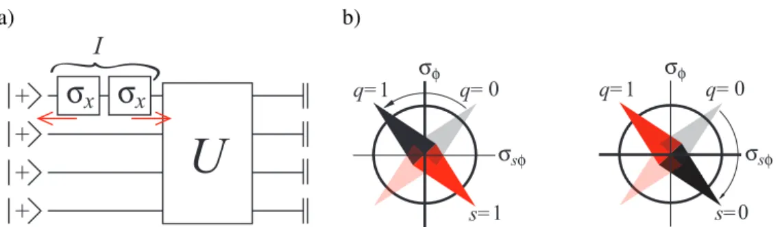
Figure 2: Two symmetry transformations. a) Gauge transformation in the circuit model. For any logical qubitl, an identity I=σx(l)σx(l) is inserted into the circuit next to the input. The leftσx is propagated

backwards in time, and absorbed by the input state _|+_i. The right σx is propagated forward in time,

flipping rotation angles and, potentially, measurement outcomes in the passing. b) Flipping a measure-ment plane in MBQC. In the measuremeasure-ment plane[σφ,σsφ], the Pauli operatorσφ is distinguished over

σsφ because the rule for adjusting a local observableOfor measurement isO[q=1] =σφO[q=0]σ_φ†.

If, for a qubita,Taa=0 (withT the influence matrix) then the exchangeσ_φ(a)_←→σ_s(a)_φ is a symmetry transformation for the given MBQC.

the quantum register in the initial stateNn

i=1|+ii, (2) unitary evolution composed of, say, CNOT gates

and one-qubit rotations about theX- andZ-axes, and (3) local measurements for readout. Such a circuit is displayed in Fig. 2 above. Then, into every qubit line individually, we may insert an identityI=σxσx

next to the input; See Fig. 2. The leftσx is propagated backwards in time until absorbed by the input

state_|+_i. The rightσxis propagated forward in time, flipping rotation angles and readout-measurement

outcomes in the passing.

This transformation is anequivalence transformation, since it is caused by the insertion of an identity gate into the circuit of Fig. 2. It changes the sign for certain rotation angles, i.e. when angles are counted positive or negative. Specifically, for thez-rotation gates next to each input qubit we can individually choose our convention for which rotation angles are called positive or negative, respectively. Once those signs are fixed on the input side, they are fixed throughout the circuit. Changing this reference affects the procedure of computation, but leaves the distribution of computational results unchanged. We therefore call it a gauge transformation.

3.2 The gauge transformations in the measurement-based model

Translating the above discussed gauge transformations from the circuit model into MBQC it is easily seen that the above relations Eq. (8) and (13) are incomplete. We find the more general relations

q=Ts+Hg mod 2, (15a)

o=Zs+Rg mod 2, (15b)

withga choice of gauge.

However, the presence of the extra terms in the processing relations strengthens their interdependence with the resource state, which is the reason why we discuss them here.

We may now want to derive the generalized processing relations Eq. (15a,15b) directly in MBQC, without reference to the circuit model. Before discussing the general case, we return to the specific example of the three-qubit cluster state in Section 2.2.

Example: Consider the productK1K3=σ_φ(1)⊗σ_φ(3)ofK1,K3 in Eq. (6). When used in Eq. (5), the

effect of this stabilizer element is to flip the measurement bases of qubits 1 and 3. Hence, the relation Eq. (14) generalizes to





q1

q2

q3



=





0 0 0

1 0 0

0 1 0



 



s1

s2

s3



+





1 0 1



g₁ mod 2. (16)

This is precisely what one would expect from the insertion ofσxσx next to the input of the equivalent

quantum circuit in Eq. (7).

We now turn to the general case. Via Eq. (5), the stabilizer groupS_(|Ψ_i)acts onsandq. Denote the post-measurement state of qubita_∈Ωby_|sa,qaia, withsathe measurement outcome andqaspecifying

the measurement basis. Then, as in Eq. (5),

O

a∈Ω

ahsa,qa|

!

|Ψ_i= O

a∈Ω

ahsa,qa|

!

K_|Ψ_i= O

a∈Ω

ahsa,qa|K

!

|Ψ_i, _∀K_∈S_(|Ψ_i). (17)

Sinceσs|s,qi=|s⊕1,qiandσφ|s,qi=|s,q⊕1i, for a stabilizer elementK=Na_∈Ω(σ (a)

s )va(σ_φ(a))wathe

action ofGK ons,qis

GK:

s _−→ s+v mod 2,

q _−→ q+w mod 2. (18)

Again, nothing changes by the insertion of a stabilizer (identity) operator into the state overlap of Eq. (5), and transformationsGK are therefore equivalence transformations. They can be used to constrain the possible temporal orders in MBQC, as we discuss explicitly in Appendix A.

3.3 Closed time-like curves – good or bad?

Partial temporal orders for an MBQC with a given resource stabilizer state and fixed measurement planes are the solution to two constraints, namely

1. Every qubit in the resource state musthavea forward cone3.

2. The forward cones generate an irreflexive and antisymmetric relation under transitivity.

In this paper we allow closed time like curves (CTC) in the computation; we are interested in classifying all transitivetemporal relationsconsistent with a given resource stabilizer state and set of measurement planes. We do not restrict to partial orders per se, and therefore drop the above Condition 2. The remaining Condition 1 may, at first sight, hardly seem to pose any constraints at all. However, it does. It imposes a self-consistency condition on each forward cone. As we make explicit in Section 6.2, this self-consistency condition in certain cases takes the form of a wave equation.

A temporal relation among measurements which is not a partial order contains closed time-like curves, and can be implemented in familiar linear time only by employing postselection. On the other

hand, temporal relations which contain closed time-like curves have recently been found of indepen-dent interest [32]. They are the translation of quantum circuits with post-selection CTCs [33], [34] into MBQC. We may compare with the theory of General Relativity, where certain solutions of the Einstein equations contain closed time-like curves. Such solutions give rise to a host of paradoxes, and whether they are physical is under debate [36]. But Einstein’s field equations are not abandoned because they allow for CTCs.

3.4 Correction and gauge operations in the stabilizer formalism

To state and prove our results on MBQC temporal order, we need to make a few more definitions. It turns out that the possible temporal relations, and indeed the classical processing relations Eq. (15a), (15b), can be parametrized by two subsets ofΩ, namely the computational output setOcompand the gauge input

setIgauge. We define these sets next.

We say that the measurement outcome sa of qubitaiscorrectedin a given MBQC, if by insertion

of a suitable stabilizer operatorKin Eq. (17) equivalence ofsa=1 with the reference outcomesa=0

is established, at the cost of adjustment of measurement bases and/or re-interpretation of measurement outcomes on other qubits.

We observe that if for a given MBQCallmeasurement outcomes sa,a∈Ω, can be corrected then

these measurement outcomes contain no information and no linear combination of them is worth out-putting. Thus, in general there will be a set of qubits whose measurement outcomes are not corrected.

Definition 6(Computational output set). For a given MBQC, the computational output set Ocomp⊆Ωis the set of qubits whose measurement outcomes are not corrected.

The correction operations for the qubits in a∈(Ocomp)c, c.f. Eq. (5), are each implemented by

correction operators K(a)_∈S_(|Ψ_i). For each a_∈(Ocomp)c, K(a) has the property that it flips the

measurement outcomesa at qubita, but does not flip the measurement outcome on any other qubit in

(Ocomp)c. In this way, it is ensured that the correction operation is for qubitaindividually.

Definition 7 (Correction operator). For an MBQC with a given stabilizer resource state_|Ψ_i, fixed set

Σof measurement planes and computational output set Ocomp, for each a_∈(Ocomp)c _{the corresponding} correction operator K(a)_∈S(_|Ψ_i)is a Pauli operator satisfying the conditions

K(a)_|a ∈ {σs(a),σ_s(a)_φ },

K(a)_|b ∈ {I(b),σφ(b)}, ∀b∈(Ocomp)c\a.

(19)

The correction operatorK(a)can be used to correct an “undesired” measurement outcome at qubita, c.f. Eq. (5). If, for a given operatorK(a),K(a)_|b∈ {σ_φ(b),σ_s(b)_φ }then, by Eq. (5), the measurement basis

at qubitbdepends on the measurement outcome for qubita. In terms of the influence matrixT,

K(a)_|b∈ {σ (b) φ ,σ

(b)

sφ } ⇐⇒[T]ba=1, ∀a∈(Ocomp)c,b∈Ω. (20)

Note that in the first line of Eq. (19) we allow K(a)_|a =σ_s(a)_φ only because we are admitting closed

time-like curves in the present discussion. K(a)_|a=σ_s(a)_φ means that the measurement basis for qubita

depends on the outcomesaof the measurement of qubita. This amounts to a closed time-like curve only involving qubita(self-loop) and is an obstacle to deterministic runnability.

Because the qubitsa_∈Ocomphave no correction operations,Tba=0 for allb∈Ω, and thus

Thus,Ocompand the correction operators{K(a),a∈(Ocomp)c}completely determine the influence matrix

T and hence the temporal relation among the measurements.

Conversely, ifOcompand{K(a),a∈(Ocomp)c}are unknown, then the constraints Eq. (19) pose

self-consistency conditions on them. We discuss these conditions further below.

As we have seen in the concrete three-qubit example above, for a given MBQC the relation between the choiceqof measurement bases and the measurement outcomessin general allows for an offset term

Hg, c.f. Eq. (15a). Thus, the measurement bases for a certain set of qubits can be freely chosen until the initially arbitrarygbecomes fixed. This observation leads to

Definition 8(Gauge input set). For a given MBQC with input set I, the gauge input set Igauge⊆I is a set of qubits such that for each i_∈Igaugethe parameter qi specifying the locally measured observable Oi[qi] can be freely chosen.

Analogously to the correction operations, there will be gauge operators which implement the ‘cor-rections’ of measurementbasesfor the qubits inIgauge. The definition of the gauge operators ensures that for alli_∈Igauge the correspondingqican be changed individually without changing the others.

Definition 9(Gauge operators). For an MBQC with a given stabilizer resource state_|Ψ_i, fixed setΣof measurement planes, computational output set Ocomp and gauge input set Igauge, for each i∈Igauge, the corresponding gauge operator K(i)_∈S(_|Ψ_i)is a Pauli operator satisfying the conditions

K(i)_|i = σ_φ(i),

K(i)_|j = I(j), ∀j∈(Igauge∩(Ocomp)c)\i, K(i)_|k ∈ {I(k),σφ(k)}, ∀k∈((Igauge)c∩(Ocomp)c)\i, K(i)_|l ∈ {I(l),σs(l)}, ∀l∈(Igauge∩Ocomp)\i.

(22)

Like previously for the correction operations, Eq. (22) poses self-consistency condition on the possi-ble setsIgaugeand{K(i),i∈Igauge}.

Lemma 1. The correction operators K(a) of Eq. (19), a_∈(Ocomp)c, and the gauge operators K(i)of Eq. (22), i_∈Igauge, are independent. That is, for all sets J ⊂Igauge, L⊂(Ocomp)c with J6= /0∨L6= /0,

˜

K(J,L):=∏_i∈JK(i)∏_a∈LK(a)₆=I(Ω).

Proof of Lemma 1. (indirect) Assume that there exists a pair J,L, with J 6= /0_∨L6= /0, such that ˜

K(J,L) =I(Ω). Then, for allb_∈(Ocomp)c, ˜K(J,L)|b=1. Now, with Eq. (19), K(b)|b∈ {σs(b),σ_s(b)_φ },

andK(c)_|b∈ {σφ(b),I(b)} for allc∈(Ocomp)c\b. With Eq. (22), K(i)|b∈ {σφ(b),I(b)}for all i∈Igauge.

Therefore, no otherK(_·),K(_·)can cancel aσs(b)-contribution fromK(b)to ˜K(J,L). Hence,b6∈Lfor all b_∈(Ocomp)c, and thusL= /0. By an analogous argument, noK(·) can cancel theσ_φ(i)-contribution of

K(i)to ˜K(J,L), hencei_6∈Jfor alli_∈Igauge, andJ=/0. Thus, ˜K(J,L) =I(Ω)=⇒J,L=/0. Contradiction.

Hence, theK(a),K(i)are independent.

Remark: For any given MBQC with fixed temporal relation, the computational output setOcompis a

subset of the output setO, see Eq. (21). ButOcompandOare not necessarily equal. Likewise,Igauge⊆I

by definition, butIgauge andI may not be equal. To illustrate this point, we consider the following two

examples.

Example 1. Consider the 3-qubit cluster state of Section 2.2, with measurement planes[X/Y]for all three qubits. We consider the correction operatorsK(1) =K2, K(2) =K3 for qubits 1 and 2, and

respectively. As was discussed previously for the above choice of correction operations, I=_{1_} and

O=_{3_}. Thus, in the present exampleIgauge=IandOcomp=O.

Example 2. Consider a Greenberger-Horne-Zeilinger state_|GHZ_i= (_|000_i+_|111_i)/√2 as resource state, with all three qubits measured in a basis in the[X,Y]-plane. We use the stabilizer elementsK(1):=

Z1Z3=σs(1)σs(3)andK(2):=Z2Z3=σs(2)σs(3)as correction operations for qubits 1 and 2, andK(1):= X1X2X3=σ_φ(1)σ_φ(2)σ_φ(3)as gauge operator. Then, the choiceIgauge={1}andOcomp={3}is admitted by

Eqs. (19) and (22), respectively. On the other hand, this is an example of a temporarily flat MQC,T =0. Therefore,I=O=_{1,2,3}, andOcomp6=O,Igauge6=I.

Lemma 2. For any MBQC on a stabilizer state,|Igauge| ≤ |Ocomp|.

We prove Lemma 2 in Section 3.5.

Definition 10. A pair Igauge, Ocompis called extremal iff|Igauge|=_|Ocomp|.

As will become clear in the next section, extremal pairsIgauge,Ocompare easier to handle than general

pairs, and are not very restrictive (c.f. Theorem 2).

We still need to relate the classical output vectoroappearing in Eq. (15b) to the setOcomp. To this

end, we make the following

Definition 11 (Optimal classical output). A classical output vector o, with processing relations o= Zs+Rg, is optimal iff the following conditions hold

1. Maximality: Upon left-multiplication by an invertible matrix, Z can be brought into a unique normal form

Z_∼(Z_{|I), (23)}

where the column split is between(Ocomp)c|Ocomp, and

2. Determinism:For the matrixZ_{in Eq. (23),}

[Z_{]i j=1⇐⇒K(j)|i∈ {σs}(i)_,σ(i)

sφ}. (24)

In other words Eq. (24) informs us that the jth column ofZ_{is simply the restriction of the support of} K(j)toOcomp.

The reason for defining an ‘optimal classical output’ besides a ‘classical output’ is the following: One could, in principle, run an MBQC perfectly deterministically and then chooseosuch that nothing is outputted at all, or all outputted bits, independent of the measurement angles chosen, are zero guar-anteed or perfectly random guarguar-anteed. The above definition of an optimal classical output eliminates such choices. Maximality says that there is one bit of optimal output per qubit ofOcomp. The

deter-minism condition can be understood from the correction procedure explained in Eq. (5). For a qubit

j_∈(Ocomp)c, we account for the undesired outcome sj =1 by inserting K(j) into the state overlap hϕloc|Ψi=hϕloc|K(j)|Ψi. Now consider a qubit i∈Ocomp. By Eq. (23),si contributes to the output

bitoi, thei-th bit ofo. If K(j)|i∈ {σs(i),σ_s(i)_φ}, then the insertion ofK(j)into the overlap flipssi, i.e., si−→si⊕1. This needs to be taken into account when reading out si. The linear combinationsj⊕si

remains unaffected by the correction forsj.

3.5 Normal form of the resource state stabilizer

Let us briefly review which pieces of information specify an MBQC. A priori, there are four: the set of measurement angles, the setΣof measurement planes, the resource state_|Ψ_iand the classical process-ing relations Eq. (15a,15b). The measurement angles entirely drop out of all our considerations about temporal order. Next, we observe that when specifying the measurement planes and the resource state separately, we really specify too much. Starting from a given pair_|Ψ_i,Σ of resource state and set of measurement planes, for any local Clifford unitaryU, the pairU_|Ψ_i,U(Σ) obtained by applyingU to both the measurement planesΣand the stabilizer state_|Ψ_iis again a valid pair, i.e., it consists of a set of a stabilizer state and a set of measurement planes. Furthermore, it amounts to exactly the same com-putation as the original pair. The pair_|Ψ_i,Σis thus redundant. To remove this redundancy, we combine the measurement planes and the stabilizer state _|Ψ_i into the stabilizer generator matrixG_(|Ψ_i) in the σφ/σs-stabilizer basis,

G_(|Ψ_i) = (Φ_||S). (25)

Therein, the columns to the left (right) form theσφ (σs-) part of the stabilizer generator matrix. G(|Ψi)

comprises all information from the resource state_|Ψ_iand the set of measurement planesΣrelevant for the discussion of MBQC. We do not need to know the state and the measurement planes separately.

Now note that the correction operatorsK(a),a_∈(Ocomp)c, and the gauge operatorsK(i),i∈Igauge,

are all elements of the stabilizerS(_|Ψ_i), and, by Lemma 1, are independent. Thus, they either form or can be completed to a set of generators forS(_|Ψ_i). This observation leads us to the following

Lemma 3. For any MBQC on a stabilizer state_|Ψ_iwith extremal Igauge, Ocomp, the generator matrixG

ofS_(|Ψ_i)can be written in the normal form

G ∼₌

σφ σs

Igauge (Igauge)c(Ocomp)cOcomp



 

0 TT _I ZT

I HT 0 RT





.

(26)

The matricesH_, R_, T_, Z _{are related to the matrices H, R, T , Z governing the classical processing of} measurement outcomes in MBQC,q=Ts+Hg mod 2ando=Zs+Rg mod 2, via

T =

0 0

T ₀

, H=

I H

,Z= Z_{|I ,R=}R_{. (27)}

Proof. By Definition 7, a correction operator K(a) exists for every a_∈(Ocomp)c. By Eq. (19) these

operators have no support inI _⊇Igauge and are|(Ocomp)c|in number and must take the following form:

0 A I B , where theσφ part is split asIgauge,Igaugec while theσs-part is split asOcomp,(Ocomp)c.

The gauge operators are, by definition, of the form: I C 0 D , where the column splits are as for the correction operators. Since there are_|Ω_|generators for the stabilizerG(_|Ψ_i), of which_|(Ocomp)c|are

already accounted for, there can be at most_|Ocomp|independent gauge operators, i.e.,|Igauge| ≤ |Ocomp|

these two sets of generators exhaust the stabilizer generators and we can write the stabilizer as

G_(|Ψ_i) =

Igauge (Igauge)c(Ocomp)cOcomp



  

0 A I B

I C 0 D



  

,

(28)

for suitable matricesA,B,C andD. We now need to identify these matrices. By definition,Igauge⊆I.

Measurement outcomes on qubitsa_∈Ocompare not corrected, hence f c(a) = /0 for alla∈Ocomp, and

Ocomp⊆Ofollows from the definition of the output setO. Then, the influence matrixT takes the form

T =

0 0

T ₀

, (29)

where the column split is(Ocomp)c|Ocompand the row split isIgauge|(Igauge)c. Now consider the correction

operatorK(a)fora_∈(Ocomp)c in the upper part ofG(|Ψi)in Eq. (28). We already know from Eq. (20),

that theσφ part ofK(a)is the forward cone ofa. Therefore we must haveA=TT. Further comparing,

with Eq. (24) which states that the restriction of theσspart of the correction operatorK(a)toOcompis

theath column ofZ_{. But this is precisely theath row ofB, thus we infer thatB=}ZT_.

Next, consider row iof the lower part of G_(|Ψ_{i)in Eq. (28). Row iis(0, ..,0,1,0, ..,0|}cT_||0|dT_).

The corresponding stabilizer operatorK(i), when inserted into the overlap_hϕloc|Ψi as in Eq. (5), flips

the measurement basis at qubitiand of qubitsl_∈(Igauge)cwith[c]l=1. It further flips the measurement

outcomes at qubitsm∈Ocompwith[d]m=1. Therefore,

H=

I H

, with H_=CT_,and

R=R_{, with} R_=DT_.

We thus arrive at the normal form Eq. (26).

4

Interdependence of resource state and temporal order

Let us return to our discussion from the beginning of Section 3.5, on which pieces of information are needed to describe an MBQC. At this stage, apart from the set of measurement angles which do not enter our discussion, we remain with two pieces of data specifying a given MBQC, namelyG(_|Ψ_i)and the processing relations Eq. (15a), (15b). But it doesn’t stop there. As the results of [14], [15], [16] show, the resource state_|Ψ_i, the measurement planesΣand the influence matrixT—being part of the classical processing relations Eq. (15a), (15b)—are not independent. Specifically, given the setsI of first-measurable andOof last-measurable qubits in addition to_|Ψ_iandΣ, the temporal order (generated byT) can be worked out completely.

A further question is whether the temporal relations compatible with a resource state_|Ψ_iand set of measurement planesΣfit into a common framework. In this regard, we show that the classical processing relations (containing the temporal order) for MBQC with a fixed resource state and set of measurement planes, for extremal pairsIgauge,Ocomp, are in one-to-one correspondence with the bases ofG(|Ψi), c.f.

Theorem 3.

4.1 Results

We now present four theorems on the mutual dependence of the resource state and the classical process-ing relations.

Theorem 1. Consider an MBQC on a stabilizer state_|Ψ_{i, with fixed measurement planes and an}

ex-tremal pair of gauge input set Igaugeand computational output set Ocomp. Then, the relationsq=Ts+Hg

mod 2, ando=Zs+Rg mod 2for an optimal outputoare unique.

That is, once the resource state _|Ψ_i, the measurement planes andIgauge, Ocomp are fixed, there is

no freedom left to choose the classical processing relations. They are uniquely determined by the for-mer. In particular, for fixed stabilizer state _|Ψ_i and measurement planes, T =T(Igauge,Ocomp), H=

H(Igauge,Ocomp)etc.

A corollary of Theorem 1 is that given the measurement planes and an extremal pairIgauge,Ocomp, the

resource state_|Ψ_iuniquely determines the influence matrixT. One may ask how restrictive a condition the extremality of the pairIgauge,Ocompis. In this regard, note

Theorem 2. Consider an MBQC on a fixed resource stabilizer state for fixed measurement planes, with an influence matrix T and input and output sets I(T), O(T), such that no qubit a_∈Iccan be individually gauged with respect to I(T), O(T). Then, there exists an extremal pair Igauge⊆I, Ocomp⊆O such that T =T(Igauge,Ocomp).

The input setI(T)and the output setO(T)which appear in Theorem 2 are uniquely specified byT

through Definition 5.T(Igauge,Ocomp)is uniquely specified by the pairIgauge,Ocompthrough Theorem 1.

Theorem 2 states that all temporal relations for an MBQC, subject to the extra condition on the qubits which can be individually gauged, arise from extremal pairsIgauge,Ocomp. By establishing Theorem 2

we trade the condition of the pairsIgauge,Ocompbeing extremal for the condition that no qubit inIccan

be individually gauged. The latter is a more meaningful condition. Suppose a qubita inIc could be individually gauged wrtI,O. ThenK(a) exists. For anybwithK(b)_|a=σ_φ(a), ˜K(b):=K(b)K(a)is a

valid correction operator for qubitb, and ˜K(b)_|a=I(a). Hence, acould be removed from all forward

cones and thereby be made a qubit in I. By imposing the extra condition in Theorem 2, we exclude temporal relations where certain qubits could be in the input setI but aren’t.

Theorem 1 is mute on the question of which extremal pairsIgauge,Ocompare admissible. Theorem 3

below describes how much freedom remains for the choice of the classical processing relations, given

G_(|Ψ_i).

Theorem 3. For MBQC with a fixed resource stabilizer state _|Ψ_i and fixed measurement planes, the classical processing relations for extremal Igauge, Ocomp, as specified by the matrices H, R, T , Z and the sets Igauge,Ocomp, are in one-to-one correspondence with the bases of the matroidG(_|Ψ_i).

Theorem 4. Consider an MBQC on a stabilizer state|Ψ_{i, with classical processing relations}q=Ts+ Hg mod 2, o=Zs+Rg mod 2 for an optimal classical output o, such that rk H =rk Z. Then the classical processing relations uniquely specify the stabilizer generator matrix G_(|Ψ_i) in the σφ/σs -basis, i.e. the resource stabilizer state|Ψ_{iand set}Σ_{of measurement planes up to equivalence.}

Remark: For Theorem 4 it does not matter whether or not the classical processing relations codify a temporal relation which is a partial order.

Remark: There is a constructive procedure for obtaining G(_|Ψ_i) (in theσφ/σs-basis) from the linear

processing relations. If the processing relation did not stem from an actual computation but rather was “made up”, the resultingG_(|Ψ_i)may not be a valid stabilizer generator matrix. I.e., the rows ofG_(|Ψ_i) may correspond to Pauli operators which do not pairwise commute.

4.2 Proofs of Theorems 1-4

Theorem 1 is an immediate consequence of Lemma 3.

Proof of Theorem 2. Assume thatIis valid input set andOis a valid output set for a given MBQC. Then, the stabilizer generator matrix of the resource state can be written in theσφ/σs-basis as

G(_|Ψ_i) =

I Ic Oc O



  

0 T˜T I A

B C 0 D



  

, (30)

for some matricesA,B,CandD. The influence matrixT can be obtained as

TT =

0 T˜T

0 0

, (31)

with the column split betweenIandIc, and the row split betweenOcandO. The matricesBand(B_|C)do not necessarily have maximal row-rank. By row transformations of(B|C||0_|D)we extract the dependent rows, and obtain

G_(|Ψ_i) =

I Ic Oc O



          

0 T˜T _{I A}

0 0 0 D′

0 C′′ 0 D′′

B′′′ C′′′ 0 D′′′



          

, (32)

However, note that each row in the third set of rows in the above matrix can either be interpreted as a correction operatorK(a), with non-empty forward cone f c(a), for somea_∈O, or a gauge operatorK(i) for somei_∈Ic_{. The former is ruled out because everya∈Omust have an empty forward cone. The}

SinceG(_|Ψ_i) has full row rank, so does the matrixD′ appearing in Eq. (32). We may then choose a set ∆O_⊆O such that the columns of D′ indexed by ∆Oform a maximal independent set. We set

Ocomp:=O\∆O. Then, by further row transformations which do not affect ˜T, the matrix in Eq. (32) can

be converted to

G_(|Ψ_i) =

I Ic _Oc _{∆O O}

comp        

0 T˜T I 0 _A′

0 0 0 I A′′

B′′′ C′′′ 0 0 D′′′

        . (33)

B′′′has full row rank by construction. We can therefore find a setIgauge⊆Isuch that the columns ofB′′′

indexed byIgauge form a maximal independent set. For any such setIgaugewe can convert the matrix in

Eq. (33) fully into the normal form Eq. (26) without affectingT.

For any of the above choices forIgauge⊆IandOcomp⊆O, the resulting influence matrixT(Igauge,Ocomp)

can be extracted as

T(Igauge,Ocomp)T =





0 T˜T

0 0

0 0



, (34)

with the column split between I and Ic, and the row split between Oc, ∆Oand Ocomp=O\∆O. By

comparison of Eqs. (31) and (34) we verifyT =T(Igauge,Ocomp).

Remark: Comparing Eq.(33) with the normal form in Eq. (26), we can write the stabilizer matrix in a slightly varied form that can be useful later.

G_(|Ψ_i) =

Igauge ∆I Ic Oc ∆O Ocomp

        

0 0 T˜T I 0 ZT

1

0 0 0 0 I ZT

2

I HT

1 HT2 0 0 RT

         , (35)

whereZ= (Z₁|Z₂)_{and where}HT = (HT

1|HT2).

Proof of Theorem 3. Denote by B _{the set of bases of} G_{, and by}T _{the set of extremal classical}

pro-cessing relations of form Eq. (15a), (15b), specified by the triple(Igauge,Ocomp,{H,R,T,Z}). Then, the

mapping h:B_−→T exists and is a bijection. (1) Existence of h: By the normal form Eq. (26) of

G _{= (}Φ_||S), for a given basisB(G_{)the setsIgaugeandOcompare extracted as follows. A qubitiis inIgauge}

if and only if the corresponding column ofΦappears in B(G_{). A qubitais inOcompif and only if the}

corresponding column ofSdoes not appear inB(G). KnowingIgaugeandOcomp,{H,R,T,Z}is uniquely

determined via Theorem 1. (2) Surjectivity ofh: By definition of “extremal”. (3) Injectivity ofh: given

IgaugeandOcomp,B(G) = Φ|Igauge|SOcomp

is unique.

Proof of Theorem 4. We divide the proof into the following steps: i) First, with rkH=rkZ, the process-ing relations stem from an extremal pairIgauge,Ocomp. We show that given an extremal pairIgauge,Ocomp,

From these matrices we can derive the corresponding normal form of the resource state uniquely. Let us denote this byN _{. In iii) and iv) we show that the following diagram commutes, which establishes the}

equivalence of normal forms of all extremal pairs.

(Igauge,Ocomp)

Λ

−−−−→ (I_gauge′ ,O′

comp)

  y

T_,H_,Z_,R

  yT

′_,H′_,Z′_,R′

N _{−−−−→}M(Λ) N′

(36)

In Eq. (36),M(Λ)is a transformation on the normal formN _{, dependent on}Λ. Because of their inde-pendence, we consider the transformationsIgauge →Igauge′ andOcomp→O′compseparately in iii) and iv)

respectively.

i) ExtractingH_,R_,T_andZ_{: Given any set of inputsIand outputsOby Theorem 2, we know that there}

always exists an extremal pair(Igauge,Ocomp), whereIgauge⊆I,Ocomp⊆O. By Eq. (29),Tis uniquely

specified byT. By the assumption of the classical output being optimal,Zcan be brought into the unique normal form of Eq. (23) by left multiplication with an invertible matrix and (permuting the columns if necessary),Z_{can be extracted. The matrixH may not appear in Eq. (15a) in its normal}

form Eq. (27), nonetheless for an invertible matrix Λ, the vector q specifying the measurement bases is invariant underH _−→HΛ, g_−→Λ−1_{g. By definition ofI}

gauge, every qubit inIgauge can

be individually gauged with respect toIgauge, Ocomp. Therefore, (up to row permutations), we can

chooseΛsuch that

HΛ=

I H

, (37)

where the row split is betweenIgauge(upper) and(Igauge)c(lower).ΛandHare unique. The classical

outputois invariant under the transformationR−→RΛ′_,g−→(Λ′₎−1_{g. However, since Eqs. (15a)}

and (15b) refer togin the same basis,Λ′is now fixed:Λ′=Λ. Then,R_=RΛ, with theΛof Eq. (37). ii) Assembling the normal form: Using the unique matrices H_, R_, T_, Z_{, by Lemma 3, we can now}

assemble the normal form Eq. (26) of the stabilizer generator matrix for the resource state_|Ψ_i. By assumption of Theorem 4, the matricesH,R,T,Zdescribe a valid computation, and the normal form Eq. (26) derived from them must thus yield a valid description of a quantum state. In particular, all Pauli operators specified by the rows ofG(_{H,R,T,Z})_{in Eq. (26) must commute. (The rows are}

independent by design of the normal form.) We have thus constructed a description of_|Ψ_i. SinceH_, R_,T_,Z_{are unique, so is|}Ψ_i.

We now proceed to construct the stabilizerS(_|Ψ_i) from the processing relations whenIgauge and

Ocomp are not specified. From the classical processing relation Eq. (15a) we can still extract the

input setIand the output setO, by testing which rows and columns ofT identically vanish. Then, the possible choices forIgaugeandOcompare limited toIgauge⊆IandOcomp⊆Oby definition.

iii) Equivalence underΛ:Igauge→Igauge′ . In order to prove this we rely on the slightly variant version

of the normal form ofG_(|Ψ_i)as shown in Eq. (35) which also includes additional detail about the correction operators. As noted above, the different normal forms forH can be interconverted by right-multiplication with an invertible matrixΛ(change of basis forg), i.e.H,R_−→HΛ,RΛ, where

HT = (I_|HT_{). Under such a transformation, the upper part of the normal form Eq. (26) for}G_(|Ψ_i) remains unchanged, and the lower part is transformed(HT_||0|RT_)−→ΛT_(HT_||0|RT_{). Invertible}

iv) Equivalence underΛ:Ocomp→O′comp. Proving that a different choice ofOcompdoes not change the

stabilizer state is a little more complicated. We proceed in the following manner. From Theorem 3, we know thatIgauge∪Occomp are the bases of a matroid. Therefore for two distinct computational

output setsOcompandO′′comp, there exists another computational output setOcomp′ =Ocomp\{i}∪{j},

wherei_∈Ocomp\O′′compand j∈O′′comp\Ocomp. Therefore, it suffices if we show that the stabilizer

state does not change if we change the computational output set fromOcomptoO′comp. Assume that

the classical relation for the computational output setOcompis given as

o=Zs+Rg= (Z_1|Z_2|I)s+R_{g. (38)}

where the column split ofZ is betweenOc_comp, ∆O, and Ocomp. The corresponding normal form

(with the column split inσφ-partIgauge|Igaugec ) is





0 T˜T _{I 0} ZT

1

0 0 0 I ZT

2

I HT _{0 0} RT



, (39)

whereTT =

_˜

TT

0

. Suppose that we transformOcomptoOcomp\ {i} ∪ {j}, wherei∈Ocompand

j_∈∆O. Without loss of generality assume that i is the last column ofZ_{2. (It cannot be an all}

zero column because, then it would not be possible for it to be inOcomp.) LetZ1=

xT ZA

and

Z₂₌

aT 1

ZB b

. ThenΛ=

1 0

b I

acting onZachieves the transformationOcomptoO′comp.

Λ(Z_1|Z_{2|I) =}

xT aT 1 1 0

ZA+bxT ZB+baT 0 b I

(40)

∼

xT aT 1 1 0

ZA+bxT ZB+baT b 0 I

= (Z′

1||Z′2||I) (41)

We claim that this same transformation can be effected by row transformations ofG(_|Ψ_i). First let us focus on the middle set of rows inG_(|Ψ_i), namely the correction operators for∆O. Then acting

byM(Λ) =

I a

0 1

gives us

M(Λ)(0_||0_|I|ZT

2) =

0 0 I a 0 Z_BT+abT

0 0 0 1 1 bT

(42)

∼

0 0 I 0 a Z_BT+abT

0 0 0 1 1 bT

= (0_||0_|I_|Z′T

2 ). (43)

Now if take the last row in Eq. (43), namely(0_||0_|0_|1_|bT) =cand addxcto the top set of rows in Eq. (39) we obtain

0 T˜T _{I 0 x 0 Z}T A+xbT

∼ 0 T˜T _{I 0} Z₁′T ₍₄₄₎

showing the equivalence ofZ_andZ′_{. The equivalence of}R_andR′_underΛcan be shown in exactly the same fashion as forZ_1andZ′

1.