The influence of macroeconomic factors to the dynamics of stock exchange in the republic of Kazakhstan

For citation: Ekonomika regiona [Economy of Region]. — 2016. — Vol. 12, Issue 4. — pp. 1263–1273 doi 10.17059/2016–4–26

УДК 336.76

S. U. Niyazbekova a), I. E. Grekov b), T. K. Blokhina a) a) _{Peoples Friendship University of Russia (Moscow, Russian Federation; e-mail: shakizada.niyazbekova@gmail.com)}

b) _{Orel State University named ater I. S. Turgenev (Orel, Russian Federation)}

THE INFLUENCE OF MACROECONOMIC FACTORS TO THE DYNAMICS

OF STOCK EXCHANGE IN THE REPUBLIC OF KAZAKHSTAN

This article describes the inluence of macroeconomic factors on Kazakhstan Stock Exchange Market by using data from 2005 to 2014. Engle-Granger cointegration test has shown that stock index is cointegrated with the exchange rate, interest rate, CPI and oil price. Vector error correction model has conirmed that mac-roeconomic variables and the stock index has a long-term equilibrium relationship. Moreover, empirical re-sults have shown that stock index can be used as a leading indicator of the economic situation in Kazakhstan. Therefore, the authors decided to consider the impact of major macroeconomic indicators to the dynamics of the stock market of the Republic of Kazakhstan. The Engle-Granger cointegration test results show that the following variables such as exchange rate, 10-years long-term bond rate, the consumer price index and the Brent oil price are cointegrated with stock index, which means that there is a long-term relationship between this stock market index and these variables. With the help of econometric models, the authors have found the factors such as the exchange rate, the 10-year long-term bonds rate, the consumer price index and the Brent oil price (these factors have the long-term relationship with stock market index). Changes in the dynamics of the stock market index in Kazakhstan are caused by changes in the dynamics of Central bank's reserves and export. The analysis has shown that the economy of the Republic of Kazakhstan (the index relects the situa-tion in the real sector of the economy) remains dependent on world oil prices, the volume of exports and the rate of the national currency.

Keywords: bank, capital, economic, inance, money, stock, index, market, price, value, efect, balance

1. Introduction

In recent years, in post-Soviet countries, there is active work on the development of stock mar-kets, as one of the most important mechanisms for the low of capital. It can be seen or assumed that in the post-Soviet countries with raw oriented economy, the growth of the stock market is inlu-enced by external factors instead of internal fac-tors. That is why we decided to consider the im-pact of major macroeconomic indicators to the dynamics of the stock market of the Republic of Kazakhstan as one of the post-Soviet countries.

Considering how some factors may affect the asset price, it would be logical to assume that there are speciic ways on which this factors can operate. The price of any asset can be evaluated through dividend discount model (DDM), which

had been proposed by Miller and Modigliani [1]. According to the idea of this model, the price of any asset as well as stock price is equal to the pres-ent value of future cash lows of the asset (stock, bond). As an asset is stream of cash lows from business perspective and value of an asset equals to the value of stream of cash lows,

1 _{© Niyazbekova S. U., Grekov I. E., Blokhina T. K. Text. 2016.}

( )

(

)

t t E C

P

r =

+

∑

where tE

t(C) — expected cash lows of an asset in

period; 1/(1 +r)t — discount factor at the _t period;

r< 1 — discount rate.

Changes of asset (stock, bond and other assets) price is a combination of changes in expected fu-ture cash lows and discount rates

( )

( )

(

)

dE C d r

dP

P E C r

+

=

-+ (2)

A number of empirical studies inform that the impact of all factors somehow affects to the expected future cash lows or discount rate. According to these empirical studies, there is a re-lationship between macroeconomic variables and changes in assets prices or equity market returns.

2. Literature review 2.1. Industrial production index

Industrial production index (IP), is the index

of real production output. According to the em-pirical studies with monthly data, industrial pro-duction has been often used instead of GDP since

GDP data is available on a quarterly or annual ba-sis. Growth of the industrial production index is calculated as

( )

log(IPt+ ) log- IPt , (3) where IP — Index of industrial production.

Fama [2, p. 545–565, р. 1089–1108] and James [3, p. 1375–1384] showed that the expected growth of the industrial production index has a signiicant positive effect on stock prices growth. Fama (1990) [3, р. 1089–1108] revealed that the growth rate of future production output describes the variation of 6 % growth in equity market prices. He notes that the past and current values of output growth rates affect the future values.

Kaul [5, p. 253–276] estimates the variation in stock returns due to expectations of future cash lows by regressing stock returns on future growth rates of real economic activity. He found that in-dustrial production explains as much more var-iation as alternative real activity variables, but growth rates of real GNP and gross private invest-ment are close competitors.

Schwert, among others, found that large frac-tions of annual stock return variances can be traced to forecasts of real economic variables such as real GNP and industrial production (IP) [6,

p. 1237–1257]. These authors and the others have shown that the relation between stock returns and future real activity is strong. Geske and Roll have conirmed that stock returns are highly correlated with future real economic activity. These facts in-dicate that real economic activity really shows or explains the stock market return, on the other hand, there is an inverse relation between stock market return and economic activity that is why stock market index called a good leading indicator for future production [7, p. 1–33].

Esen Erdogan, Umit Ozlaly in the study of the impact of macroeconomic factors on the Turkey stock market showed a positive relationship be-tween the industrial production index and stock market. The authors explained this relationship as the growth of industrial production that leads to an increase in income and cash lows of companies that have a positive trend on the stock market re-turn [8, p. 69–90].

Luo and Visaltanachoti in their work, based on general equilibrium model proposed by them, indicated two possible channel impact of output on stock index return: demand shock and impact of relative prices [9]. The first channel operates as an increase in production of domestic goods caused by shock in demand for them is accom-panied by the improvement of trade conditions with foreign markets. These improvements and

growth in output generate an upward pressure on the domestic financial market. Thus, there is a positive relationship. On the other hand, the relative prices channel may lead to the op-posite effect. If the release of traded goods in a foreign market is growing regarding the release of non-tradable goods, then the relative price of non-tradable goods begins to rise which will lead to increase in the exchange rate and the deterioration of trade conditions. Deteriorating conditions have downward pressure on the do-mestic financial market.

Tsuma in her work explored the link between the stock index and the index of industrial produc-tion and consumer prices. The author found that there is a stable relationship between industrial production and stock indices [10]. However, a sign of relationship is not deined as the different lags of the index of industrial production has different effects.

In addition, previous studies have shown a signiicant positive relationship between the in-crease in prices and the expected growth of indus-trial production and an insigniicant link with the past performance of the industrial production.

2.2. Exchange rate

The study of the impact of exchange rates on the stock market returns as well as stock index price is important to the economists, international inves-tors and politicians. Thus, as for international in-vestors, it is due to the fact that the positive corre-lation between the exchange rate and stock mar-ket increases volatility in the yield, while negative relationship can eliminate the need to hedge cur-rency risk. There have been a number of empiri-cal studies conducted to test the relationship be-tween stock prices and exchange rates using dif-ferent techniques and databases, but the results were mixed.

of the exchange rate inluences on the stock mar-ket in different directions.

On the other hand, the "stock-oriented" models of exchange rates offered by Branson and Frankel claim that innovation in the stock market affect to aggregate demand through the wealth effect and the effect of liquidity, thereby, inluencing on the demand for money (Gavin.) For example, the stock price decline leads to a reduction of do-mestic investors’ wealth, leading to a decrease in the demand for money with a consequent reduc-tion in interest rates. Subsequently, the low-inter-est rates prevent capital inlows, given other con-ditions being equal, which leads to currency de-valuation and, consequently, the dynamics of the exchange rate may be affected by changes in stock prices.

Esen Erdogan and Umit Ozlaly showed the am-biguous relationship between the exchange rate and the stock market in Turkey. So until 1994, the depreciation of national currency led to a reduc-tion of the dynamics of the stock market, however, after that period, the connection became opposite. On the one hand, the depreciation of the national currency leads to higher prices for imported cap-ital goods, reducing proit margins, on the other hand, increases the competitiveness of irms in in-ternational markets, which lead to an increase in stocks.

Maria Caporale, John Hunter, Menla Ali inves-tigated the nature of the relationship between the stock market and exchange rates in the US, UK, Canada, Japan, Euro Zone and Switzerland using data from 2007 to 2010. The two-dimen-sional UEDCC-GARCH model showed unidirec-tional Granger causality, i.e. change the dynam-ics of the stock market led to a change in the ex-change rate of the US and UK and communica-tion in the opposite direccommunica-tion in Canada, as well as bi-directional causality in the Eurozone and Switzerland. The results of unsteady correlations showed that the relationship between two varia-bles increased during the last inancial crisis. The authors' conclusions indicate the limited oppor-tunities for investors to diversify their portfolios during the crisis, due to a general drop in prices and the depreciation of currencies [12, p. 87–103]. Chen’s empirical results (2011) showed that the relationship between exchange rates and stock prices in Asia also became stronger in times of crisis due to the low of capital. During the crisis, foreign investors sell stocks, resulting in an out-low of capital and puts pressure on national cur-rencies. In addition, Chen held a sectoral analy-sis of the causal link, which showed that the par-allel between the dynamics of the exchange rate

and export-oriented industries are not so strong. This indicates that the parallel between the dy-namics of exchange rates and the Asian emerging stock markets is generally caused by the move-ment of capital rather than the trade balance [13, p. 383–403].

2.3. Interest rate

There are many theoretical studies about the impact of interest rates on the value of the stock price, and through them to the consolidated stock indexes.

Here are the main ones:

— Interest rates affect the stock price through the discounting factor (Campbell, 1987). The gen-eral level of interest rates determines the yield, which wants to receive by investing in stocks, that is — the discount rate. The value of the stocks de-pends on the yield to maturity rate: the higher yield, investors want to get from the ownership of stock, the less they want to buy them. Accordingly, there is a negative correlation — the lower gen-eral level of interest rates, the higher will be the stock price. Thus, the interest rate relects the loss (proit) on alternative investments [14, p. 373–399];

— The interest rate relects the marginal pro-ductivity of capital. The interest rate is the re-turn on invested capital. In equilibrium, interest rate equal to the marginal productivity of capital. Consequently, the low rate indicates a low capital productivity, which affects the mood of investors and reducing the demand for the stocks, which in turn leads to lower prices;

— Interest rates determine the amount of bor-rowing. Low-interest rates allow companies to save, reduce borrowing costs and thus, to increase its proits, which leads to the higher prices of stocks.

On the other hand, a large number of stud-ies show a positive relationship between inter-est rates and stock prices. Apergis and Eleftheriou conducted an empirical study examining the re-lationship between the prices of stocks, inlation and interest rates on monthly data in Greece in the period 1988–1999. The results have shown that although interest rates are positively cor-related with stock prices, this relationship is not statistically signiicant [16, p. 231–236]. Bohl et al. studied the relationship between stock returns and short-term interest rates in Germany for the period 1985–1998. They found a positive but sta-tistically insigniicant relationship between stock returns and short-term interest rates on daily and monthly data [17, p. 719–733].

Durr and Giot explored the possibility of a long-term relationship between income, prices, stocks and interest rates, deined as the rate on long-term government bonds using the cointegra-tion analysis for 13 countries in the period from January 1973 to December 2003. Their empirical results have shown that long-term rates on gov-ernment bonds statistically signiicant effect on the stock market [18, p. 613–641].

2.4. Money supply

There are two competing hypotheses about the relationship between the money supply and stock market returns. Milton Friedman suggests that balanced investor portfolio has several types of in-cluding money. A sudden increase or decrease in the growth rate of money supply leads to an im-balance in the investment portfolio. The increase in the money supply in line with the income ef-fect leads to the fact that investors increase de-mand for other assets. This hypothesis implies that the reaction of the price of other assets to the change in the money supply is shown with a cer-tain lag. The alternative hypothesis of market ef-iciency (EM) suggests that all relevant informa-tion immediately and fully relected in the mar-ket value of the stock exchange. Accordingly, the increase in money supply will immediately affect the stock market.

Sprinkel carried out the irst attempt to em-pirically test the hypothesis of MP. Using data for 1918–1960 years, he graphically displayed the level of money supply and the dynamics of the stock market. He made a conclusion that changes in the stock market lag behind changes in the money supply [19]. Palmer updated Sprinkel’s data of 1960–1969 and came to the same conclusion. EM hypothesis was irst proposed by Fama [20, p. 19–22]. Subsequently, Rozeff (Rozeff), using data from 1916–1972 showed empirical evidence that

static market lag effect of changes in monetary policy on stock prices almost zero. He suggests that stock prices immediately relect changes in monetary policy and, moreover, the stock mar-ket actually provides for the future growth of the money supply [21, p. 245–302].

In the works of Homa and Jaffee, the effect of money supply on the price of shares is considered from three perspectives: the impact on dividends and their growth rate, the impact on the risk-free rate and the impact on the risk premium [22, p. 1045–1066].

The main channel of inluence of money sup-ply on dividends are current and expected corpo-rate earnings. The decline in the money supply will lead to higher interest rates, which reduce the sensitivity to the percentage of costs (example, capital). Cost reduction will reduce the company's revenue and proits. It affects not only the current dividend but also lowers expectations for their fu-ture growth. The impact of money supply on the risk-free rate is positive. Reducing the money sup-ply will lead to an increase in the risk-free rate and the rationing of credit rates on the borrowed funds. In turn, that will lead to an increase in the discount rate and its expected value.

The impact on the risk premium should be con-sidered from the standpoint of the relationship to the risk of a particular investor. Risk-averse vestor requires a positive risk premium, which in-creases with increasing uncertainty regarding fu-ture dividends. If you touch the effect of money supply on the risk premium there can be a two-fold relationship. If money supply growth is not accompanied by an increase in the rate of inla-tion, the risk premium will decrease. However, if money growth is accompanied by rising inlation the risk premium will also increase.

Schwert, Pierce and Roley also consider the relationship between the money supply and the yield of inancial assets. Authors give two pos-sible explanations for the relationship between these parameters. The irst relates to the fact that economic agents expect inlation if there is an increase in money supply. The second possi-ble explanation is based on the fact that a change in the money supply, economic agents expects any action from the state regulator (such as the Central Bank). In particular, the growth of money supply agents can expect an increase in short-term interest rates, aimed at reducing the attrac-tiveness of money and curb possible inlation. Thus, changes in the proitability of inancial as-sets are a reaction to the actions of the authori-ties [23, p. 3–12].

— Stock prices only react to unexpected changes in the money supply;

— Market participants are treated as changes in the level of money supply and unexpected changes;

— The reaction of prices is symmetrical with respect to the sign of change in the money supply;

— The reaction of prices is not linear;

— The most of the reaction is shown in the irst day after the announcement of news.

2.5. Oil price

In general, the nature of the relationship be-tween the world oil prices and the stock market is determined by which the countries are exporter or importer. In the irst case in a number of research results indicate a positive association and in the second — the negative.

The research of Chen, Roll and Ross for the US market was found that the changes in oil prices have little effect on stock prices. In later stud-ies, the results were different [24, p.383–403]. The work of Cole and Jones were obtained to con-irm the presence of the negative impact of rising oil prices on the stock market. And in addition to the US market, they considered such countries as Great Britain, Canada and Japan. They also showed that the US and Canadian markets are rational: changes in stock indexes response to changes in oil prices can be completely described by the im-pact of oil prices on the current and expected fu-ture real cash lows.

In the study of Kilian and Park was received the same result. They explain it this way. Higher oil prices often relect investor concern about the fu-ture shortage of this energy. Thus, a sharp increase in the price of oil leads to the formation of the cor-responding negative sentiment on the market re-sulting in a decrease of prices [25, p. 1267–1287]. Arora, Tyers and Akram (2009) in their works indi-cate a possible connection of inancial assets and the price of oil. The authors believe that the rise in share price, evidence of the growth of production in general, and leads to an increase in demand for energy, particularly oil [26, p. 142–150].

Fedorova, Snyatkova and Sutyagin (2012) in their study conducted Granger’s test that showed a causal relationship between the index of devel-oping countries and oil prices. This is understand-able high demand in developing countries for en-ergy resources. Rising oil prices slow economic ac-tivity in emerging markets [27, p. 41–49]. Fedorova and K. Pankratov have tested econometric model EGARCH, to assess the impact of various factors on the Russian stock market. The analysis re-vealed a strong dependence of the dynamics of the

MICEX index on the oil price and the dollar ex-change rate [28, p. 78–83].

Fedorova E. A. and Lazarev M. P. used the monthly data determine the impact of changes of oil prices on the stock market of the Russian Federation, which have been divided into two pe-riods: the general and the crisis. With the help of the causal Granger’s test; evaluation of the VAR model; cointegration analysis, the authors showed that oil prices have a long-term impact on the Russian stock market [29, p. 11–14].

2.6. Inlation

On the one hand, increased inlation may neg-atively affect the stock market, as the acceleration of inlation reduces the value of expected cash lows, increases the nominal interest rate, and, as a result, the discount factor. This, in turn, leads to a decrease in the stock price. On the other hand, the rise in prices increases the revenue of the com-pany which has a positive effect on cash lows re-lated to the shares and increases their value.

Some early articles (Fama; James) distinguish the effects of the impact of the expected and un-expected inlation on stock returns and show a statistically signiicant negative relationship be-tween inlation and stock returns. Fama (1981) de-ined the expected inlation as

1 1 ,

 t t t t

i = a + b_- TB_- + η (4)

where a_{t - 1} — arandomwalk, TB_{t - 1} — continuously

compounded inlation rate and the rate on short-term bills. The calculated values a_{t - 1}+ bTB_{t - 1}

rep-resent expected inlation, and remnants of the re-gression ηt, — an unexpected inlation.

70 years showed a signiicant negative relation-ship between inlation and the price of the shares, since in these years in the United States observed two-digit inlation, caused by the policy of re-ducing unemployment [31, p. 67–140]. Similarly, Bond and Webb (1995) revealed the presence of a negative relationship between inlation and the price of shares in the period of hyperinlation [32, p. 327–334].

In addition to the existence of "tax effect" should highlight the presence of another ef-fect — "the illusion of inlation." Inlation ad-versely affects to the expectations regarding fu-ture cash lows, which is connected with the al-ready mentioned tax effect, and with the planning of the nominal interest rate. This may lead to an underestimation of the shares, that is, it turns out that inlation has a negative effect on the value of shares in companies, and through them to the Composite Stock Index. Cohen and Modigliani (Modigliani, et al., 1979) hypothesized that in a period of inlation, investors underestimate the share of about 50 %. At the heart of this underes-timation are two main reasons. The irst is that in-vestors in planning their activities do not use real and nominal interest rate, which is signiicantly higher [33, p. 24–44]. Second — already described the tax effect. Ritter and Warr (Ritter, et al.) have shown that this effect is actually observed in par-ticular from 1982 to 1999. US investors have con-sistently underestimated the shares [34, p. 29–61]. Hess and Lee in their work provided a brief summary of earlier conclusions regarding the re-lationship between stock returns and inlation. The authors, based on the facts of earlier studies (Blanchard, et al.), argue that the two situations are possible. The irst situation is related to the supply shocks that are usually non-monetary in nature. In this case, inlation arises is usually neg-atively associated with stock returns. On the other hand, demand shocks are usually caused by mon-etary shocks [35, p. 1203–1218]. In this case, the link between inlation and stock returns is

posi-tive. Therefore, a sign the relationship between in-lation and stock returns depends on what shocks are stronger in a given time.

3. Hypothesis

Based on the analysis of empirical studies and the structure of the stock index KASE following hypotheses have been put forward (see Result).

4. Research methodology 4.1. Unit Root Test

In order to do time series analysis, it is required to check them for stationarity since the model re-sults will be unreliable if series are non-station-ary. A unit root test will be used to avoid spuri-ous regression. There is a variety of tests, however, we will use the most popular one (Dickey — Fuller Test) in order to check series stationarity. Null and alternative hypotheses are as follows:

H

0: ρ = 1 Unit root [Variable is not stationary];

H₀: ρ < 1 No unit root [Variable is stationary].

If a coeficient markedly differs from 1, i.e. be-low 1, the hypothesis presuming у to contain a unit root is rejected. Rejection of null hypothe-sis means series stationarity. If we do not reject a null hypothesis, we conclude the series have a unit root. If the test shows non-stationarity of time se-ries, the irst difference will be taken.

4.2. Granger Causality Test

Granger causality test has been used. The statistical test is destined for determination of cause and effect relation between the variables. Particularly, the test is based on the following bi-variate regressions

, 1   , 1 .  1   1,

S t i S t i M t t V = a + b

∑

∑

,      2 , 1    , 1   2, M t i S t i M t t

V =a + θ

∑

∑

where εi — stationary residuals.

Null hypothesis — VM is not a reason for

chang-ing. VS is rejected if li signiicantly differs from null.

Possible relation of VS to VM can be also tested, by using a joint signiicance of θ_i s. This can be done by standard F-tests. The following four results can

be obtained: causality of VM from VS, causality of VM from VS, bidirectional causality, no causality, where li≠ 0; θi ≠ 0; li ≠ 0, θi≠ 0, respectively.

4.3. The Engle-Granger Test

Engle and Granger proposed a simple cointe-gration test that implicates least-squares itting of regression of two integrated variables and test-ing of regression residuals for a unit root. So, as-sume that X

1, …, Xn are integrated variables, then

Result

Macroeconomic factors Hypothesis/ Relationship

he price of Brent crude oil Positive

Industrial production Positive

Exchange rate Positive

Interest rate Negative

CPI Negative

S&P 500 Negative

Central bank reserves Positive

Export Positive

Import Negative

X

1 is a dependent variable. Least-square itting

re-gression is

1t 1 2 2t .   n nt    .t

X = b + b X +… +b X + ε (7)

The regression is called the Engle-Granger re-gression and Engle-Granger test is a test for the presence of unit root in regression residuals. If the test shows presence of a unit root in residu-als, then the variables X

1, …, Xn are cointegrated

with cointegration vector (1, -b2- … -bn). Put it

differently,

2 2 ... .

n n n

Z=X -b X - -b X (8)

The stationary linear combination of inte-grated variables means a presence of long-run equilibrium. If regression residuals are non-sta-tionary, the variables will not be cointegrated and estimation of least-square itting will not be justiiable.

4.4. Vector error correction model (VECM)

In our study, we will use the Engle-Granger pro-cedure for building error correction model. Error correction model is a multitemporal model built on the irst-order differences of integrated varia-bles. So, when series X

t, Yt~I (1) are contegrated

— Long-run (equilibrium) relationship model

Y

t= a + bXt;

— Short-run dynamics model or error correc-tion model (ECM) these models are coherent.

Engle and Granger proposed a two-step model for building ECM for cointegrated series. At the irst stage, unknown parameters a and b are es-timated by least-square method within the regu-lar regression model yt and xt. Next, when we ob-tain estimated parameters _aˆ _{and b}ˆ_{, we ind}

esti-mated values of departure from long-run equilib-rium point, i.e. estimated regression residuals are

ˆ _ˆ ˆ _.

t t

Z=Y - a - bX (9)

At the second stage, we separately estimate the following model using least-square model:

1 11 12 1 1 1

1 1

,

m m

i i

t t i t i t t

i i

X a X_- Y_- Z

-= =

∆ = + b ∆

∑

∑

2 21 22 2 1 2

1 1

.

m m

i i

t t i t i t t

i i

Y a X_- Y_- Z

-= =

∆ = + b ∆

∑

∑

Error correction model lies in the fact that model shows the way how to adjust the short-run departures from long-short-run equilibrium. In the model above, Z is a recourse vector.

5. Empirical results 5.1. Data description

In this study, we used the monthly data of main macroeconomic indicators such as inlation, in-dustrial production index, export, import, inter-est rate, exchange rate, oil prices, money supply, central bank reserves, S&P500 and KASE stock in-dex from January 2005 to December 2014. All data were taken from the Bloomberg and Thomson Reuters Eikon platforms. The total number of ob-servation is 120, which we considered as suficient for the analysis of time series.

5.2. Analysis

To conduct our analysis it is necessary to test for stationarity our time series data of selected variables:

— KASE stock index (Stock_index); — Brent Oil price (Brent);

— Consumer Price Index (CPI); — Exchange rate (EXCHRATE);

— 10-year long-term bong (YTRB) as interest rate;

— Industrial production index (INDUSTRIAL); — Central Bank reserves (CB RESERVES); — Export (EXPORT);

— Import (IMPORT); — Money supply (M3),

— US S&P500 stock index (Table 1).

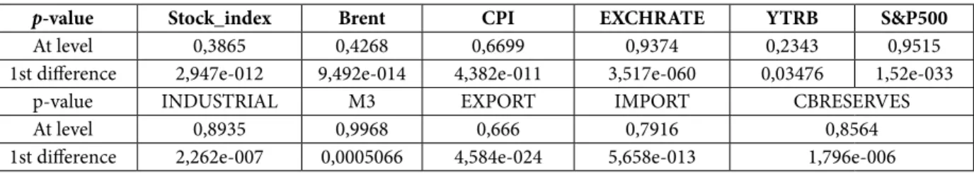
Based on stationarity test above, we were looking for the presence of a unit root in our se-ries. The result of stationarity test shows that all the series is non-stationary. However, after tak-ing irst difference they become stationary and the null hypotheses about having a unit root is rejected. Therefore, all the series are integrated of irst order, so we test for cointegration using the Engle-Granger method (Table 2). To deter-mine the lag for cointegration test we will use the cub root of the number of observation for each series.

Table 1

ADF-тест

p-value Stock_index Brent CPI EXCHRATE YTRB S&P500

At level 0,3865 0,4268 0,6699 0,9374 0,2343 0,9515

1st diference 2,947e-012 9,492e-014 4,382e-011 3,517e-060 0,03476 1,52e-033

p-value INDUSTRIAL М3 EXPORT IMPORT CBRESERVES

At level 0,8935 0,9968 0,666 0,7916 0,8564

The Engle-Granger cointegration test results show that the following variables such as ex-change rate, 10-years long-term bond rate, the consumer price index and the Brent oil price are cointegrated with stock index, which means that there is a long-term relationship between this stock market index and these variables.

As we determined the long-term relationship, next we will determine the short-term relation-ship. To check the presence of short-term rela-tionship we will use Error Correction Model. The sign and magnitude of Error Correction coeficient indicate the direction and speed of adjustment to-wards long-term equilibrium. It should be nega-tive and signiicant. The neganega-tive sign means that in the absence of changes in the independent vari-ables, the delection pattern of long-term depend-ency is adjusted by increasing the dependent vari-able. Bannerjee al. believes that a signiicant error correction factor is further proof of the existence of a stable long-term relationship (Table 3).

The estimated Error Correction coeficient EC (-1) for EXCH_RATE, YTRB, CPI, Brent was -0.033;

-0.0537; -0.05; -0.009 respectively. This means that in the absence of change in other variables deviation from the long-term equilibrium model for this factors balanced by 3.3 %, 5.4 %, 5 % and 0.9 % increase in the stock index in a month. This means that returning to the long-term equilib-rium model takes more than 30, 16, 20, 111 and 3 months respectively. As result, a regression equa-tion can be represented as follow:

STOCK_INDEX = 0,44BRENT + 110CPI + + 1,04EXCH_RATE + 18,6IND

-- 0,27YTRB - 1,7S&P500

Now we will test the series for Granger Causality test (Table 4).

Based on Granger causality test, changes in the dynamic of stock market index is caused by Brent oil price, central bank reserves and export.

However, it should be noted that the stock in-dex is an indicator of changes in the following var-iables: Industrial production index, exchange rate, central bank reserves, and exports.

6. Practical signiicance of the study

Identifying the impact of macroeconomic fac-tors on the dynamics of the stock market is im-portant for investors, as it affects the investment yield. This analysis is conducted within the frame-work of one of the stage of the fundamental ap-proaches to determining the future dynamics of the stock market. Proposed methodology allows to quantify the impact of macroeconomic factors on the stock market, and improve the accuracy of predicting the behavior of stock market indices, which is extremely important for the evaluation of investment programs. Moreover, as Granger Causality test showed KASE index can be used to predict changes in the real economy, which can help to evaluate the economic decision-making results.

7. Conclusion

This study can be concluded with the opion that several macroeconomic factors which in-luence the dynamic of the stock market index in Kazakhstan. With the help of econometric models, we found the factors, such as the exchange rate, the 10-year long-term bonds rate, the consumer price index, the Brent oil price (these factors have

Table 2

Test Engle-Granger cointegration

Engle-Granger Cointegration test (2005–2015 period)

Algorithm: equation: STOCK_INDEX(t) = a + b(i_factor)(t) + u(t).

we get the residual of the equation: u_hat(t) = STOCK_INDEX(t - aˆ -b(ˆ i_factor)(t)

ater that we check the equation ∆u_hat(t) = ϕu_t- 1 + θu_t- 1 + ζ_t to the presence of unit root H_i : ϕ = 1 without constant and trend

Variables H₀ : ϕ = 1 ϕ t_statistics P_value 10 %

Cointegrated/ No cointegration

STOCK_INDEX

EXPORT Rejected –0,0461627 –1,40723 0,1487 No cointegration

IMPORT Rejected –0,0468207 –1,61178 0,1006 No cointegration

INDUSTRIAL Rejected –0,0165552 –1,0556 0,2634 No cointegration

CB_RESERVES Rejected –0,0235813 –1,35101 0,1642 No cointegration

EXCH_RATE Rejected –0,0353227 –2,0923 0,03499 Cointegration

M3 Rejected –0,0154954 –1,19775 0,212 No cointegration

YTRB Rejected –0,0559277 –2,82718 0,004568 Cointegration

CPI Rejected –0,0502706 –2,55029 0,01043 Cointegration

SP500 Rejected –0,0247939 –1,504 0,1244 No cointegration

Table 3

Vector Error Correction model

Variables Cointegrating Vector

EC1

(p-value) IRF

EXCH_RATE 5 –11,969 −0,0334173

(0,0588 *₎

YTRB –277,84 −0,0537191

(0,0117**₎

CPI 5 –14,795 −0,0515554

(0,0137**₎

Brent 5 –16,895 −0,00928192

(0,6107)

Table 4

Granger causality test

Variables Inluence F-statistics Prob. Causality at 10 % level of signiicance

INDUSTRIAL Industrial to Srock_Index 1.38818 0.2348 Does not Granger Cause

Srock_Index to Industrial 2.33141 0.0474 Does Granger Cause

EXCH_RATE Exchange rate to Srock_Index 1.38770 0.2349 Does not Granger Cause

Srock_IndextoExchange rate 2.99116 0.0146 Does Granger Cause

YTRB YTRB to Srock_Index 0.43997 0.8197 Does not Granger Cause

Srock_Index to YTRB 0.43293 0.8247 Does not Granger Cause

CPI CPI to Srock_Index 0.93388 0.4623 Does not Granger Cause

Srock_Index to CPI 1.46636 0.2072 Does not Granger Cause

BRENT BRENT to Srock_Index 3.71492 0.0039 Does not Granger Cause

Srock_Index to BRENT 1.68034 0.1458 Does not Granger Cause

the long-term relationship with stock market in-dex). Changes in the dynamics of the stock market index in Kazakhstan is caused by changes in the dynamic of central bank's reserves and export. The analysis shows that the economy of the Republic of Kazakhstan (the index relects the situation in

the real sector of the economy) remains depend-ent on world oil prices, the volume of exports and the rate of the national currency. Changing of these factors leads to a change in return on the stock market.

Variables Inluence F-statistics Prob. Causality at 10 % level of signiicance

CB RESERVES Reservesto Srock_Index 2.73543 0.0231 Does Granger Cause

Srock_Index to Reserves 2.90980 0.0169 Does Granger Cause

EXPORT Export to Srock_Index 1.98536 0.0869 Does Granger Cause

Srock_Index to Export 3.53581 0.0054 Does Granger Cause

IMPORT Import to Srock_Index 1.16271 0.3326 Does not Granger Cause

Srock_Index to Import 1.10408 0.3628 Does not Granger Cause

M3 М3 to Srock_Index 1.50976 0.1931 Does not Granger Cause

Srock_Index to М3 0.41749 0.8357 Does not Granger Cause

End of Table 4

Acknowledgements

he study has been supported by LLP "Astana School of Business and Technology".

References

1. Miller and Modigliani (1961). Retrieved from: http://www.nzfc.ac.nz/archives/2011/papers/updated/279.pdf (date of access: 17.04.2016).

2. Fama, E. F. (1981). Stock Returns, Real Activity, Inlation, and Money.  he American Economic Review, 71(4),  545– 565.

3. Fama, E. F. (1990). Stock Returns, Expected Returns, and Real Activity.  he Journal of Finance, 45(4),  1089–1108.

4. James, C., Koreisha, S. & Partch, M. (1985). A VARMA analysis of the causal relations among stock returns, real out-put, and nominal interest rates.  Journal of Finance, 40,  1375–1384.

5. Kaul, G. (1987). Stock returns and inlation. he Role of the Monetary Sector.  Journal of Financial Economics, 18(2),  253–276.

6. Schwert, G. W. (1990). Stock returns and real activity: A century of evidence.  he Journal of Finance, 45(4),  1237–1257.

7. Geske, R. & Roll, R. (1983). he Fiscal and Monetary Linkage between Stock Returns and Inlation.  he Journal of Finance, 38(1),  1–33.

8. Erdogan, E. & Ozlale, U. (2005): Efects of macroeconomic dynamics on stock returns: the case of the Turkish stock exchange market.  Journal of economic Cooperation, 26(2),  69–90.

9. Luo and Visaltanachoti in their work (2010). Retrieved from: https://www.hse.ru/pubs/share/direct/docu-ment/63054888 (date of access: 31.01.2016).

10. Retrieved from: http://www.inesad.edu.bo/bcde2009/B3 %20Daniel%20Canedo.pdf (date of access: 31.03.2016).

11. Dornbusch and Fischer. Retrieved from: http://www.akes.or.kr/eng/papers(2013)/34.full.pdf (date of access: 01.04.2016).

12. Caporale, G., Hunter, J. & Ali, F. (2014). On the linkages between stock prices and exchange rates: Evidence from the banking crisis of 2007–2010.  International Review of Financial Analysis, 33,  87–103.

13. Chen, N., Roll, R. & Ross, S. (1986). Economic forces and the stock market.  Journal of business, 59(3),  383–403.

14. Campbell, J. Y. (1987). Stock returns and the term structure.  Journal of inancial economics, 18(2),  373–399.

15. horbecke, W. (1997). On stock market returns and monetary policy.  he Journal of Finance, 52(2),  635–654.

16. Apergis, N. & Eletheriou, S. (2002). Interest rates, inlation, and stock prices: the case of the Athens Stock Exchange.  Journal of Policy Modeling, 24(3),  231–236.

17. Bohl, M. T., Siklos, P. L. & Werner, T. (2007). Do central banks react to the stock market? he case of the Bundesbank.  Journal of Banking & Finance, 31(3),  719–733.

18. Durré, A & Giot, P. (2007). An international analysis of earnings, stock prices and bond yields.  Journal of Business Finance & Accounting, 34(3–4),  613–641.

19. Sprinkel, B. W. (1964).  Money and stock prices.  Homewood, Ill: RD Irwin.

20. Palmer, M. (1970). Money supply, portfolio adjustments and stock prices.  Financial Analysts Journal, 26(4),  19–22.

21. Rozef, M. S. (1974). Money and stock prices: Market eiciency and the lag in efect of monetary policy.  Journal of inancial Economics, 1(3),  245–302.

22. Homa, K. E. (1971). Monetary base and stock performance.  he Journal of Finance, 26(5),  1045–1066.

24. Chen, N., Roll, R. & Ross, S. (1986). Economic forces and the stock market.  Journal of business, 59(3),  383–403.

25. Kilian, L. & Park, C. (2009). he Impact of Oil Price Shocks on the U.S. Stock Market.  International Economic Review, 50(4),  1267–1287.

26. Arora, V. & Tyers, R. (2012). Asset Arbitrage and the Price of Oil.  Economic Modelling, 29(2),  142–150.

27. Fyodorova, E. A., Snyatkova, I. N. & Sutyagina Yu. N. (2012). Analiz zavisimosti mezhdu tsenoy na net, valyutnym kursom i fondovymi rynkami razvivayushchikhsya stran [he analysis of dependence between an oil price, the currency rate and the stock markets of developing countries].  Daydzhest-Finansy [Digest-Finanses], (12),  41–49.

28. Fyodorova, E. A. & Pankratov, K. A. (2009). Vliyanie mirovogo inansovogo rynka na fondovyy rynok Rossii [Impact of the world inancial market on the stock market of Russia].  Audit i inansovyy analiz [Audit and inancial analysis], (2),  78–83.

29. Fyodorova, E. A. & Lazarev, M. P. (2014). Vliyanie tseny na net na inansovyy rynok Rossii v krizisnyy period [Price inluence on oil on the inancial market of Russia during the crisis period].   Finansy i Kredit [Finances and Credit], (2),  11–14.

30. Feldstein, M. (1980). Inlation and the Stock Market.  American Economic Review, 70(5),  839–847.

31. Summers, L. H. et al. (1981). Taxation and corporate investment: A q-theory approach.  Brookings Papers on Economic Activity, (1),  67–140.

32. Bond, M. & Webb, J. (1995). Real Estate versus Financial Asset Returns and Inlation: Can a P* Trading Strategy Improve REIT Investment Performance?  Journal of Real Estate Research, 10(3),  327–334.

33. Modigliani, F. & Cohn, R. (1979). Inlation, rational valuation and the market.  Financial Analysts Journal, 35(2),  24–44.

34. Ritter, J. R. & Warr, R. S. (2002). he decline of inlation and the bull market of 1982–1999.  Journal of Financial and Quantitative Analysis, 37(1),  29–61.

35. Hess, P. J. & Lee, B. S. (1999). Stock returns and inlation with supply and demand disturbances.  Review of Financial Studies, 12(5),  1203–1218.

Authors

Shakizada Uteulievna Niyazbekova — PhD in Economics, Senior Lecturer, Peoples' Friendship University of Russia (6, Miklukho-Maklaya St., Moscow, 117198, Russian Federation; e-mail: shakizada.niyazbekova@gmail.com).

Igor Evgenievich Grekov — Doctor of Economics, Associate Professor, Head of the Department, Orel State University named ater I. S. Turgenev (29, Naugorskoe Highway, Oryol, 302020, Russian Federation; e-mail: grekov-igor@mail.ru).