The carbon budget of South Asia

(1)

BGD

9, 13537–13580, 2012

The carbon budget of South Asia

P. K. Patra et al.

Title Page

Abstract Introduction

Conclusions References

Tables Figures

◭ ◮

Back Close

Full Screen / Esc

Printer-friendly Version Interactive Discussion

Discussion

P

a

per

|

Dis

cussion

P

a

per

|

Discussion

P

a

per

|

Discussio

n

P

a

per

Biogeosciences Discuss., 9, 13537–13580, 2012 www.biogeosciences-discuss.net/9/13537/2012/ doi:10.5194/bgd-9-13537-2012

Biogeosciences Discussions

This discussion paper is/has been under review for the journal Biogeosciences (BG). Please refer to the corresponding final paper in BG if available.

The carbon budget of South Asia

P. K. Patra1, J. G. Canadell2, R. A. Houghton3, S. L. Piao4, N.-H. Oh5, P. Ciais6,

K. R. Manjunath7, A. Chhabra7, T. Wang6, T. Bhattacharya8, P. Bousquet6,

J. Hartman9, A. Ito10, E. Mayorga11, Y. Niwa12, P. Raymond13, V. V. S. S. Sarma14,

and R. Lasco15

1

Research Institute for Global Change, JAMSTEC, Yokohama 236 0001, Japan 2

Global Carbon Project, CSIRO Marine and Atmospheric Research, Canberra, ACT 2601, Australia

3

Woods Hole Research Center, 149 Woods Hole Road, Falmouth, MA 02540, USA 4

Peeking University, Beijing 100871, China 5

Seoul National University, 1 Gwanak-ro, Gwanak-gu, Seoul, South Korea 6

IPSL – LSCE, CEA CNRS UVSQ, Centre d’Etudes Orme des Merisiers, 91191 Gif sur Yvette, France

7

Space Application Centre, ISRO, Ahmedabad 380 015, India 8

National Bureau of Soil Survey and Land use Planning (ICAR) Amravati Road, Nagpur 440 033, India

9

Institute for Biogeochemistry and Marine Chemistry, 20146, Hamburg, Germany 10

National Institute for Environmental Studies, Tsukuba, Ibaraki 305-8506, Japan 11

Applied Physics Laboratory, University of Washington, Seattle, USA 12

Meteorological Research Institute, Tsukuba, Japan 13

(2)

BGD

9, 13537–13580, 2012

P. K. Patra et al.

Title Page

Tables Figures

◭ ◮

Back Close

Full Screen / Esc

Discussion

P

a

per

|

Dis

cussion

P

a

per

|

Discussion

P

a

per

|

Discussio

n

P

a

per

|

14

National Institute of Oceanography, Visakhapatnam 530 017, India 15

The World Agroforestry Centre (ICARF), Laguna 4031, Philippines

Received: 27 August 2012 – Accepted: 25 September 2012 – Published: 5 October 2012

Correspondence to: P. K. Patra (prabir@jamstec.go.jp)

(3)

BGD

9, 13537–13580, 2012

P. K. Patra et al.

Title Page

Tables Figures

◭ ◮

Back Close

Full Screen / Esc

Discussion

P

a

per

|

Dis

cussion

P

a

per

|

Discussion

P

a

per

|

Discussio

n

P

a

per

Abstract

The source and sinks of carbon dioxide (CO2) and methane (CH4) due to

an-thropogenic and natural biospheric activities were estimated for the South Asia re-gion (Bangladesh, Bhutan, India, Nepal, Pakistan and Sri Lanka). Flux estimates were based on top-down methods that use inversions of atmospheric data, and 5

bottom-up methods that use field observations, satellite data, and terrestrial

ecosys-tem models. Based on atmospheric CO₂ inversions, the net biospheric CO₂ flux in

South Asia (equivalent to the Net Biome Productivity, NBP) was a sink, estimated

at −104±150 Tg C yr−1 during 2007–2008. Based on the bottom-up approach, the

net biospheric CO₂ flux is estimated to be −191±193 Tg C yr−1 during the period

10

of 2000–2009. This last net flux results from the following flux components: (1) the Net Ecosystem Productivity, NEP (net primary production minus heterotrophic respi-ration) of−220±186 Tg C yr−1(2) the annual net carbon flux from land-use change of −14±50 Tg C yr−1, which resulted from a sink of−16 Tg C yr−1due to the establishment

of tree plantations and wood harvest, and a source of 2 Tg C yr−1 due to the

expan-15

sion of croplands; (3) the riverine export flux from terrestrial ecosystems to the coastal oceans of₊42.9 Tg C yr−1_{; and (4) the net CO}

2 emission due to biomass burning of

+44.1±13.7 Tg C yr−1. Including the emissions from the combustion of fossil fuels of 444 Tg C yr−1for the decades of 2000s, we estimate a net CO2land-to-atmosphere flux of 297 Tg C yr−1. In addition to CO2, a fraction of the sequestered carbon in terrestrial 20

ecosystems is released to the atmosphere as CH₄. Based on bottom-up and top-down

estimates, and chemistry-transport modeling, we estimate that 37±3.7 Tg C-CH4yr− 1

were released to atmosphere from South Asia during the 2000s. Taking all CO2 and

CH₄ fluxes together, our best estimate of the net land-to-atmosphere CO₂-equivalent flux is a net source of 334 Tg C yr−1

for the South Asia region during the 2000s. If CH₄ 25

(4)

BGD

9, 13537–13580, 2012

P. K. Patra et al.

Title Page

Tables Figures

◭ ◮

Back Close

Full Screen / Esc

Discussion

P

a

per

|

Dis

cussion

P

a

per

|

Discussion

P

a

per

|

Discussio

n

P

a

per

|

1 Introduction

South Asia (Bangladesh, Bhutan, India, Nepal, Pakistan and Sri Lanka) is home to 1.6 billion people and covers an area of 4.5×106km2. These countries are largely self-su_fficient in food production through wide range of natural resources, and agricultural and farming practices (FRA, 2010). However, due to rapid economic growth, fossil fuel 5

emissions have increased from 213 Tg C yr−1 in 1990 to about 573 Tg C yr−1 in 2009

(Boden et al., 2011). A detailed budget of CO₂exchange between the earth’s surface

and the atmosphere is not available for the South Asia region due to a sparse

net-work of key carbon observations such as atmospheric CO2, soil carbon stocks, woody

biomass, and CO₂uptake and release by managed and unmanaged ecosystems. Only

10

recently, Patra et al. (2011a) estimated net CO2fluxes at seasonal time intervals by in-verse modeling (also known as top-down approach), revealing strong carbon uptake of

149 Tg C month−1_{during July–September following the summer monsoon rainfall.}

The region is also very likely to be a strong source of CH4 due to rice cultivation by an amount, which still remains controversial in the literature (Cicerone and Shetter, 15

1981; Fung et al., 1991; Yan et al., 2009; Manjunath et al., 2011), and large numbers of ruminants linked to religious and farming practices (Yamaji et al., 2003; Chhabra et al., 2009). Since the green revolution there has been an increase in CH4 emissions owing to the introduction of high-yielding crop species, increased use of nitrogen and phosphorus fertilizers, and expansion of cropland areas to meet the food demands of 20

a growing human population in countries of South Asia (Bouwman et al., 2002; Patra et al., 2012a).

South Asia has also undergone significant changes in the rates of land use change over the last 20 yr contributing to the net carbon exchange. India alone has increased the extent of forest plantations by 4.5 Mha (∼7 % of 64 Mha) from 1990 to 2010 leading 25

to a 26 % increase in the carbon stock in living forest biomass (FRA, 2010).

(5)

BGD

9, 13537–13580, 2012

P. K. Patra et al.

Title Page

Tables Figures

◭ ◮

Back Close

Full Screen / Esc

Discussion

P

a

per

|

Dis

cussion

P

a

per

|

Discussion

P

a

per

|

Discussio

n

P

a

per

achieve this goal by synthesizing the results of multiple approaches that include (1) at-mospheric inversions as so-called top-down methods, and (2) fossil fuel consumption, forest/soil inventories, riverine exports, remote sensing products and dynamic global vegetation models as bottom-up methods. The comparison of independent and par-tially independent estimates from these various methods help to define the uncertainty 5

in our knowledge on the South Asia carbon budget. Finally, we attempt to separate the net carbon balance into its main contributing fluxes including fluxes from net pri-mary production, heterotrophic respiration, land use change, fire, and riverine export to coastal oceans. This effort is consistent with and a contribution to the REgional Carbon Cycle Assessment and Processes (Canadell et al., 2011; Patra et al., 2012b).

10

2 Materials and methods

The South Asia region designated for this study is shown in Fig. 1, along with the basic ecosystem types (DeFries and Townshend, 1994). A large fraction of the

area is cultivated croplands and grassland or wooded grassland (1.3×106km2 and

1.5×106km2 or 0.89×106km2, respectively). The rest of the area is classified as 15

bare soil, shrubs, broadleaf evergreen, broadleaf deciduous and mixed coniferous (0.35×106km2, 0.22×106km2, 0.11×106km2, 0.10×106km2 and 0.05×106km2, respectively). The region is bounded by the Indian Ocean in the south and the Hi-malayan mountain range in the north. The meteorological conditions over the South Asia region are controlled primarily by the movement of the inter-tropical convergence 20

zone (ITCZ). When the ITCZ is located over the Indian Ocean (between Equator to 5◦S) during boreal autumn, winter and spring, the region is generally dry without much occurrence of rainfall. When the ITCZ is located north of the region, about 70 % of precipitations occur during the boreal summer (June–September). Some of these pre-vailing meteorological conditions are discussed in relations with CO2 and CH4surface 25

(6)

BGD

9, 13537–13580, 2012

P. K. Patra et al.

Title Page

Tables Figures

◭ ◮

Back Close

Full Screen / Esc

Discussion

P

a

per

|

Dis

cussion

P

a

per

|

Discussion

P

a

per

|

Discussio

n

P

a

per

|

2.1 Emissions from the combustion of fossil fuels and cement production

Carbon dioxide emission statistics were taken from the CDIAC database of

consump-tion of fossil fuels and cement producconsump-tion (Boden et al., 2011). CO2 emissions were

derived from energy statistics published by the United Nations (2010) and processed

according to methods described in Marland and Rotty (1984). CO2emissions from the

5

production of cement were based on data from the US Department of Interior’s Geo-logical Survey (USGS, 2010), and emissions from gas flaring were derived from data provided by the UN, US Department of Energy’s Energy Information Administration (1994), Rotty (1974).

2.2 Emissions from land use and land use change

10

Emissions from land use change include the net flux of carbon between the terrestrial biosphere and the atmosphere resulting from deliberate changes in land cover and land use (Houghton, 2003). Flux estimates are based on a book keeping model that tracks living and dead carbon stocks including wood products for each hectare of land cultivated, harvested or reforested. Data on land use change was from the Global For-15

est Resource Assessment of the Food and Agriculture Organization (FAO, 2010). We also extracted information from national communication reports to the United Nations Framework Convention on Climate Change.

2.3 Fire emissions

Fire emissions for the region were obtained from the Global Fire Emissions Database 20

version 3.1 (GFEDv3.1). GFED is based on a combination of satellite information on fire activity and vegetation productivity (van der Werf et al., 2006, 2010). The former is based on burned area, active fires, and fAPAR from various satellite sensors, and the latter is estimated with the satellite-driven Carnegie Ames Stanford Approach (CASA) model.

(7)

BGD

9, 13537–13580, 2012

P. K. Patra et al.

Title Page

Tables Figures

◭ ◮

Back Close

Full Screen / Esc

Discussion

P

a

per

|

Dis

cussion

P

a

per

|

Discussion

P

a

per

|

Discussio

n

P

a

per

2.4 Transport of riverine carbon

To estimate the land to ocean carbon flux we used the six ocean coastline segments with their corresponding river catchments for South Asia as described by the COSCAT database (Meybeck et al., 2006). The lateral transport of carbon to the coast was es-timated at the river basin scale using the Global Nutrient Export from WaterSheds 5

(NEWS) model framework (Mayorga et al., 2010), including NEWS basin areas. The carbon species models are hybrid empirically and conceptually based models that

in-clude single and multiple linear regressions developed by the NEWS effort and

Hart-mann et al. (2009), and single-regression relationships assembled from the literature. Modeled dissolved and particulate organic carbon (DOC and POC) loads used here 10

(from Mayorga et al., 2010) were generated largely using drivers corresponding to the year 2000, including observed hydro-climatological forcings, though some param-eters and the observed loads are based on data spanning the previous two decade. Total suspended sediment (TSS) exports were also estimated by NEWS. Dissolved inorganic carbon (DIC) estimates correspond to weathering-derived bicarbonate ex-15

ports and do not include CO₂ supersaturation; the statistical relationships developed by Hartmann et al. (2009) were adjusted in highly weathered tropical soils (ferralsols) to 25 % of the modeled values found in Hartmann et al. (2009) to account for overesti-mates relative to observed river exports (J. Hartmann and N. Moosdorf, unpublished); adjusted grid-cell scale exports were aggregated to the basin scale using NEWS basin 20

definitions (Mayorga et al., 2010), then reduced by applying a NEWS-based, basin-scale consumptive water removal factor from irrigation withdrawals (Mayorga et al., 2010). DIC modeled estimates represent approximately 1970–2000. Overall, carbon loads may be characterized as representing general conditions for the period 1980– 2000. Carbon, sediment and water exports were aggregated from the river basin scale 25

(8)

BGD

9, 13537–13580, 2012

P. K. Patra et al.

Title Page

Tables Figures

◭ ◮

Back Close

Full Screen / Esc

Discussion

P

a

per

|

Dis

cussion

P

a

per

|

Discussion

P

a

per

|

Discussio

n

P

a

per

|

2.5 Fluxes by terrestrial ecosystem models

We use the net primary productivity (NPP) and heterotrophic respiration (RH) sim-ulated by ten ecosystem models: HyLand, Lund-Potsdam-Jena DGVM (LPJ),

OR-CHIDEE, She_ffield–DGVM, TRIFFID, LPJ GUESS, NCAR CLM4C, NCAR CLM4CN,

OCN and VEGAS. The models used the protocol as described by the carbon cy-5

cle model intercomparison project (TRENDY) (Sitch et al., 2012; Piao et al., 2012; dgvm.ceh.ac.uk/system/files/Trendy protocol%20 Nov2011 0.pdf), where each model was run from its pre-industrial equilibrium (assumed at the beginning of the 1900s) to

2009. We present net ecosystem productivity (NEP=NPP−RH) from two simulation

cases; S1: where models consider change in climate and rising atmospheric CO₂

con-10

centration, and S2: where models consider change in atmospheric CO2concentration

alone.

The historical changes in atmospheric CO₂ concentration for the period of 1901–

2009 were derived from ice core records and NOAA atmospheric observations (Keeling and Whorf, 2005). For the climate forcing datasets, monthly climate data for the period 15

of 1901–2009 from CRU-NCEP datasets with a spatial resolution 0.5◦

×0.5◦ (http:// dods.extra.cea.fr/data/p529viov/cruncep/) were used. Information on land use change was derived from HYDE 3.1 land cover dataset (Goldewijk, 2001, fftp://ftp.pbl.nl/../../ hyde/hyde31 final/). These models do not include lateral fluxes of C exported away from ecosystems (from soils to rivers, biomass harvested products) nor fluxes resulting 20

from forest and agricultural management.

We performed correlation analyses between detrended net carbon flux and two cli-mate drivers, annual temperature and annual precipitation, in order to diagnose the modeled interannual response of net carbon fluxes to these drivers (positive for carbon source, negative for carbon sink). The detrended fluxes were calculated by removing 25

(9)

BGD

9, 13537–13580, 2012

P. K. Patra et al.

Title Page

Tables Figures

◭ ◮

Back Close

Full Screen / Esc

Discussion

P

a

per

|

Dis

cussion

P

a

per

|

Discussion

P

a

per

|

Discussio

n

P

a

per

2.6 Atmospheric inverse models

The biospheric (non-fossil CO2) CO2 fluxes are available from state-of-the art atmo-spheric inversion models from the TransCom database at IPSL/LSCE (http://transcom. lsce.ipsl.fr; Peylin et al., 2012). Estimated fluxes from the following models are in-cluded in this analysis: C13 CCAM, C13 CCAM, Carbontracker EU, Jena s96 v3.2, 5

JMA 2010, LSCE an v2.1, LSCE var v1.0, NICAM MRI, RIGC TDI64, TransCom-L3 mean. We also obtained regional specific inversion results for South Asia using the CARIBIC (Schuck et al., 2010) data in the upper troposphere over India and Pakistan, which is subsequently validated using the CONTRAIL (Machida et al., 2008) data of vertical profiles over Delhi and upper troposphere over Asia (Patra et al., 2011a). CON-10

TRAIL observations are also used for inversion, with CARIBIC data for validation (Niwa

et al., 2012). Measurements of atmospheric CO2 in the South Asia region are limited

to Cabo de Rama, India for the period of 1993–2002 (Bhattacharya et al., 2009). This

site constrains the CO2 fluxes from India during winter to spring seasons only. Thus

the use of aircraft measurements is indispensible for top-down flux estimates over the 15

full seasonal cycle.

2.7 Methane fluxes

Top-down estimates: global distributions of CH4 emissions are prepared using site scale field measurements, inventories (in the case of fossil CH4emissions and livestock emissions) and their extrapolation using remote sensing of wetland distribution and 20

terrestrial ecosystem models (e.g. Mathews and Fung, 1987; Olivier and Berdowski, 2001; Ito and Inatomi, 2012). Components of these bottom-up estimations are scaled and used as an input to chemistry-transport models and compared with atmospheric mixing ratio measurements, or are used as prior flux estimates for inverse modeling of surface CH4fluxes (Patra et al., 2011a; Bousquet at al., 2006 and references therein). 25

Patra et al. (2011b) prepared 6 distinct CH₄ budgets; 5 of those being anthropogenic

(10)

BGD

9, 13537–13580, 2012

P. K. Patra et al.

Title Page

Tables Figures

◭ ◮

Back Close

Full Screen / Esc

Discussion

P

a

per

|

Dis

cussion

P

a

per

|

Discussion

P

a

per

|

Discussio

n

P

a

per

|

wetlands (Ringeval et al., 2010; Ito and Inatomi, 2012), biomass burning (van der Werf et al., 2006), and those from Fung et al. (1991), and one being based on inversion of atmospheric concentrations (Bousquet et al., 2006).

Bottom-up estimates for India:methane fluxes for India were estimated using bottom-up inventory data which relied on SPOT Vegetation NDVI, Radarsat Scan SAR (SN2) 5

and IRS AWiFS to map the different rice lands and generate the feed/fodder area for

livestock consumption (Manjunath et al., 2011; Chhabra et al., 2009).

3 Results and discussion

3.1 Emissions from fossil fuels and cement production

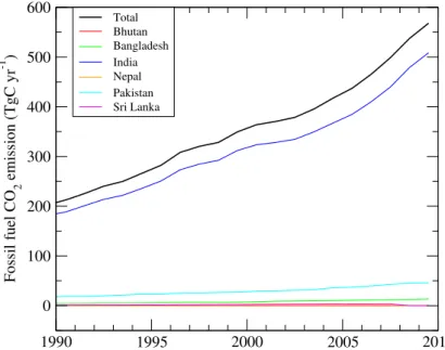
Figure 2 shows the fossil fuel and cement CO2emissions trends over the South Asia

10

region and member countries over the past two decades. Growth rates are calcu-lated as the slope of a fitted linear function, normalized by the average emissions for the period of interest. The average regional total emissions are estimated to be 278 and 444 Tg C yr−1for the periods of 1990s and 2000s, respectively. The regional total emissions have steadily increased from 213 Tg C yr−1in 1990 to 573 Tg C yr−1in 2009. 15

About 90 % of emissions from South Asia are due to fossil fuel consumptions in India

at a normalized growth rate of 4.7 % yr−1 for the period of 1990–2009. The decadal

growth rates do not show significant differences between the 1990s (5.5 % yr−1) and 2000s (5.3 % yr−1

) for the whole region, while an increased rate of consumptions was observed after 2005 (6.8 % yr−1). This acceleration (Fig. 2) in fossil fuel consumption 20

(11)

BGD

9, 13537–13580, 2012

P. K. Patra et al.

Title Page

Tables Figures

◭ ◮

Back Close

Full Screen / Esc

Discussion

P

a

per

|

Dis

cussion

P

a

per

|

Discussion

P

a

per

|

Discussio

n

P

a

per

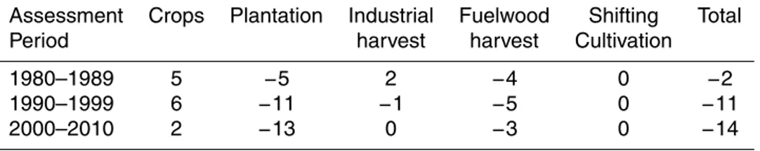
3.2 Emissions from land-use change (LUC)

The annual net flux of carbon from land-use change in South Asia was a small sink (−11 Tg C yr−1for the 1990s and−14 Tg C yr−1for the period 2000–2009) (Table 2). The average sink over the 20-yr period 1990–2009 was −12.5 Tg C yr−1. Three activities drove this net sink: establishment of tree plantations (−13 Tg C yr−1in the most recent 5

decade), wood harvest (−3 Tg C yr−1), and the expansion of croplands (2 Tg C yr−1). Wood harvest results in a net sink of carbon because both industrial wood and fu-elwood harvesting have declined recently, while the forest ecosystem productivity re-mained constant.

Tree plantations (eucalyptus, acacia, rubber, teak, and pine) expanded by 10

0.2×106ha yr−1in the 1990–1999 period and by 0.3×106ha yr−1during 2000–2009 in the region (FRA, 2010). Uptake of carbon as a result of these new plantations, as well

as those planted before 1990, averaged−11 and −13 Tg C yr−1 in the two decades,

respectively.

Industrial and fuelwood harvest (including the emissions from wood products and 15

the sink in regrowing forests) was a net sink of−6 and−3 Tg C yr−1in the two decades, most of this sink from fuelwood harvest. The net sink attributable to logging suggests that rates of wood harvest have declined in recent decades, while the recovery of forests harvested in previous years drives a net sink in forests.

The carbon sink in expanding plantations and growth of logged forests was offset

20

only partially by the C source from the expansion of croplands, which is estimated to have released 6 Tg C yr−1_{and 2 Tg C yr}−1_{during the 1990s and the first decade of 2000,} respectively.

The net change in forest area in South Asia was zero for the decade 1990–1999 and

averaged 200 000 ha yr−1 _{during 2000–2009 (FRA, 2010). Given the rates of}

planta-25

tion expansion during these decades (200 000 ha yr−1in the 1990–1999 period and by

(12)

BGD

9, 13537–13580, 2012

P. K. Patra et al.

Title Page

Tables Figures

◭ ◮

Back Close

Full Screen / Esc

Discussion

P

a

per

|

Dis

cussion

P

a

per

|

Discussion

P

a

per

|

Discussio

n

P

a

per

|

The large changes in forest area, both deforestation and afforestation, lead to gross emissions (∼120 Tg C yr−1) and a gross uptake (∼135 Tg C yr−1) that are large relative to the net flux of 14 Tg C yr−1. Thus, the uncertainty is greater than the net flux itself. The uncertainty is estimated to be 50 Tg C yr−1, a value is somewhat less than 50 % of the gross fluxes.

5

The net flux for South Asia was determined to a large extent by land-use change (the expansion of tree plantations) in India, which accounts for 72 % of the land area of South Asia, 85 % of the forest area, and >95 % of the annual increase in planta-tions. Although 11 estimates of the net carbon flux due to land use change for India published since 1980 have varied from a net source of 42.5 Tg C yr−1 to a net sink of 10

−5.0 Tg C yr−1. The recent estimates by Kaul et al. (2009) for the late 1990s and up to 2009 suggest a declining source/increasing sink (Table 2), consistent with the findings reported here for all of South Asia.

Because India represents the largest contribution to land-use change in South Asia, and because there have been a number of analyses carried out for India, the discussion 15

below focuses on India. A major theme of carbon budgets for India’s forests has been the roles of tree plantations versus native forests. The 2009 Forest Survey of India (FSI) reported a 5 % increase in India’s forest area over the previous decade. This is a net change, however, masking the loss rate of native forests (0.8 % to 3.5 % per year) and a large increase in plantations (eucalyptus, acacia, rubber, teak, or pine trees) 20

(∼5700 km2to∼18 000 km2per year) (Puyravaud et al., 2010).

The same theme is evident in the earlier carbon budgets for India’s forests. Ravin-dranath and Hall (1994) noted that, nationally, forest area declined slightly (0.04 %, or 23 750 ha annually) between 1982 and 1990. At the state level, however, adding up only those states that had lost forests (still an underestimate of gross deforestation), the 25

loss of forest area was 497 800 ha yr−1 _{between 1982 and 1986, and 266 700 ha yr}−1

between 1986 and 1988. These losses were obviously offset by “gross” increases in

(13)

BGD

9, 13537–13580, 2012

P. K. Patra et al.

Title Page

Tables Figures

◭ ◮

Back Close

Full Screen / Esc

Discussion

P

a

per

|

Dis

cussion

P

a

per

|

Discussion

P

a

per

|

Discussio

n

P

a

per

Similarly, Chhabra et al. (2002) found a net decrease∼0.6 Mha in total forest cover for India 1988–1994, while district-level changes indicated a gross increase of 1.07 Mha and a gross decrease of 1.65 Mha. These changes in area translated into a decrease of 77.8 Tg C in districts losing forests and an increase of 81 Tg C in districts gaining forests (plantations) during the same period. It seems odd, though not impossible, that carbon 5

accumulated during this period while forest area declined. Clearly, the uncertainties are high.

This analysis did not include shifting cultivation in South Asia, but Lele and Joshi (2008) attributed much of the deforestation in northeast India to shifting cultivation. Houghton (2007) also omitted the conversion of forests to waste lands, while Kaul 10

et al. (2009) attribute the largest fluxes of carbon to conversion of forests to croplands and wastelands. It seems unlikely that forests are deliberately converted to wastelands. Rather, wastelands probably result either from degradation of croplands (which are then replaced with new deforestation) or from over-harvesting of wood.

Fuelwood harvest, and its associated degradation of carbon stocks, and even de-15

forestation, seems another primary driver of carbon emissions in South Asia. For ex-ample, Tahir et al. (2010) report that the use of fuelwood in brick kilns contributed to deforestation in Pakistan, where 14.7 % of the forest cover was lost between 1990 and 2005.

In Nepal, Upadhyay et al. (2005) attribute the loss of carbon through land-use change 20

to fuelwood consumption and soil erosion, and Awasthi et al. (2003) suggest that fu-elwood harvest at high elevations of Himalayan India may not be sustainable. On the other hand, Unni et al. (2000) found that fuelwood harvest within a 100-km radius of two cities showed both conversion of natural ecosystems to managed ones and the reverse, with no obvious net reduction in biomass. They inferred that the demand for 25

(14)

BGD

9, 13537–13580, 2012

P. K. Patra et al.

Title Page

Tables Figures

◭ ◮

Back Close

Full Screen / Esc

Discussion

P

a

per

|

Dis

cussion

P

a

per

|

Discussion

P

a

per

|

Discussio

n

P

a

per

|

carbon stocks will decline (forest degradation) and may ultimately be lost entirely (de-forestation).

3.3 Emissions from fires

South Asia is not a large source of CO2 emission due to biomass burning as per

the GFED3.1 (Global Fire Emission Database, version 3.1; van der Werf et al., 2006, 5

2010). Out of about global total emissions of 2,013±384 Tg C yr−1 due open fires as detected by the various satellites sensors, 47±30 Tg C yr−1 (2.3 % of the total) only

are emitted in the South Asian countries. The average and 1σ _{standard deviations}

are calculated from the annual mean emissions in the period 1997–2009. The total emission is reduced to 44±13 Tg C yr−1if the period of 2000–2009 is considered. The 10

total fire emissions can be attributed to agriculture waste burning (14±4 Tg C yr−1), deforestation fires (21±11 Tg C yr−1), forest fires (2.6±1.5 Tg C yr−1), savanna burn-ing (4.8±1.9 Tg C yr−1) and woodland fires (1.8±1.0 Tg C yr−1) for the period of 2000– 2009. The seasonal variation of CO2emissions due to fires is discussed in Sect. 3.7.

Fire emissions due to agricultural activities will be largely recovered through the an-15

nual cropping cycles, and emissions from wildfires in natural ecosystems will be also largely recovered through regrowth over multiple decades (unless there is a fire regime change for which we have no evidence). For these reasons, carbon emissions from fires from the GFED product will not be used to estimate the regional carbon budget, given that fire emissions associated with deforestation are already included in the land 20

use change flux presented in this study. GFED fire fluxes are use to interpreted inter-annual variability.

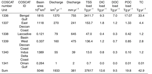
3.4 Riverine carbon flux

The total carbon export from South Asian rivers was 42.9 Tg C yr−1, with COSCAT ex-ports ranging from 0.01 to 33.4 Tg C yr−1 _{for the period of 1980–2000 (Table 4).} Con-25

(15)

BGD

9, 13537–13580, 2012

P. K. Patra et al.

Title Page

Tables Figures

◭ ◮

Back Close

Full Screen / Esc

Discussion

P

a

per

|

Dis

cussion

P

a

per

|

Discussion

P

a

per

|

Discussio

n

P

a

per

(Cole et al., 2007; Batin et al., 2009), rivers in the South Asia region contribute about 7 % of global riverine carbon export, which is more than twice the world average rate (the South Asia has about 3 % of the global land area). The largest riverine carbon export was observed from the Bengal Gulf COSCAT, which is dominated by the com-bined Ganges-Brahmaputra discharge. The riverine carbon exports from the other five 5

remaining COSCAT basins were lower by up to two orders of magnitude, ranging from only 0.01 to 4.4 Tg C yr−1(Table 4).

Because large riverine carbon loads can be due to large basin area, we also provide the basin carbon yield (riverine carbon load per unit area, excluding PIC). Basin car-bon yields varied by a few orders of magnitude, ranging from 0.04 to 18.4 g C m−2yr−1. 10

The largest basin carbon yield was again from the Bengal Gulf COSCAT. However, Laccadive Basin COSCAT and West Deccan Coast COSCAT also released 9.5 and 8.2 g C m−2yr−1, respectively. The global mean terrestrial carbon yield can be calcu-lated by dividing the global riverine carbon export of 611 Tg C yr−1

(Aufdenkampe et al., 2011; Battin et al., 2009) by the total land area of 149 million km2, providing a global 15

mean yield of 4.1 g C m−2yr−1. Therefore, the three COSCAT regions in South Asia re-leased more carbon per unit area than the global average. Considering that riverine carbon export is heavily dependent on discharge, this is not surprising since the three COSCAT regions have annual discharge values 40 to 120 % larger than the global average discharge to the oceans of 340 mm yr−1_{(Mayorga et al., 2010).}

20

The three COSCAT regions with the largest basin carbon yields (Bengal Gulf, Lac-cadive Basin, and West Deccan Coast) also corresponded to the area of highest NPP of the South Asia (Kucharik et al., 2000), consistent with areas of cultivated crops and forested regions (Fig. 1). This suggests that terrestrial inputs of carbon to the river system of the region can be a significant factor next to the riverine discharge.

25

(16)

BGD

9, 13537–13580, 2012

P. K. Patra et al.

Title Page

Tables Figures

◭ ◮

Back Close

Full Screen / Esc

Discussion

P

a

per

|

Dis

cussion

P

a

per

|

Discussion

P

a

per

|

Discussio

n

P

a

per

|

POC contribution (Table 4). Riverine TSS (Total Suspended Sediment) loads and basin yields were also the largest from the Bengal Gulf COSCAT, indicating the strong corre-lation between POC and TSS.

The carbon emitted by soils to rivers headstreams can be degassed to atmosphere as CO2or deposited into sediment during the riverine transport from terrestrial ecosys-5

tem to oceanic ecosystem (Aufdenkampe et al., 2011; Cole et al., 2007). The estimated carbon release to the atmosphere from Indian (inner) estuaries (1.9 Tg C yr−1; Sarma et al., 2012) is relatively small compared to the total river flux of South Asia region. The mosoonal discharge through these estuaries have a short residence time of OC, which helps the OC matters to be transported relatively unprocessed to the open/deeper 10

ocean. The average residence time during the monsoonal discharge period is less than a day, as observed over the period of 1986–2010, with longest residence time of 7 days for the years of low discharge rate (Acharyya et al., 2012). On an average the processing rate of OC in estuaries is estimated to be 30 % in the Ganga-Brahmaputra river system in Bangladesh, and the remaining 70 % are stored in the deep water of 15

Bay of Bengal (Galy et al., 2007).

3.5 Modeled long-term mean ecosystem fluxes from biosphere models

Bottom-up estimates from all ten ecosystem models, forced by rising atmospheric CO₂

concentration and changes in climate (S2 simulation), agree that terrestrial ecosys-tems of South Asia acted as a net carbon sink during 1980–2009. The average mag-20

nitude of the sink (NEP) estimated by the ten models is −210±164 Tg C yr−1, rang-ing from −80 Tg C yr−1 to −651 Tg C yr−1. Rising atmospheric CO2 alone (S1

simu-lation) accounts for 89 %-110 % of the carbon sink estimated in the CO2+Climate

simulations (S2), suggesting a dominant role of the CO₂ fertilization e_ffect in

driv-ing the regional sink. The decadal average NEPs are −193±136, −217±174 and

25

−220±186 Tg C yr−1, respectively, for the 1980s, 1990s and 2000s. The net

pri-mary productivity (NPP) for the same decades are 2117±372, 2160±372 and

(17)

BGD

9, 13537–13580, 2012

P. K. Patra et al.

Title Page

Tables Figures

◭ ◮

Back Close

Full Screen / Esc

Discussion

P

a

per

|

Dis

cussion

P

a

per

|

Discussion

P

a

per

|

Discussio

n

P

a

per

Five of the eight models providing CO₂+Climate simulations (S2) show that climate change alone led to a carbon source of 0.1 Tg C yr−1

to 63 Tg C yr−1

over the last three

decades (the difference between simulation S2 and S1); the three other models (OCN,

ORC and TRI) show that climate change enhanced the carbon sink by−14, −6 and

−4 Tg C yr−1. Such model discrepancies result in average net carbon flux driven by 5

climate change is near neutral (10±22 Tg C yr−1).

3.6 Modeled long-term mean ecosystem fluxes from inversions

Top-down estimates of land–atmosphere CO2 biospheric fluxes (i.e. without fossil fuel emissions, and inclusive of LUC flux and Riverine export) are estimated by using

at-mospheric CO2concentrations and chemistry-transport models. Results are available

10

from 11 atmospheric inverse models participating in the TransCom intercomparison project with varying time period between 1988–2008 (Peylin et al., 2012). The inver-sions were run without any observational data over the South Asia region for most part of the 2000s. Therefore, we place a very low confidence in the TransCom inversion results, and a medium confidence in the results of two additional regional inversions 15

using aircraft measurements over the region. The estimated net land–atmosphere CO2

biospheric fluxes from the two regional inversions are−317 and−88.3 Tg C yr−1

(Pa-tra et al., 2011a; Niwa et al., 2012). The range of biospheric CO₂ fluxes estimated

by the 11 TransCom inversions is−158 to 507 Tg C yr−1, with a median value being

a sink of−35.4 Tg C yr−1with a 1-σstandard deviation 182 Tg C yr−1. The median of the 20

TransCom inversions is chosen for filtering the effect of outliers values. In summary, for this RECCAP carbon budget, we propose as a synthesis of the inversion approach the mean value of the two “best” inversions using region-specific CO2data and the median

of TransCom models (−147±150 Tg C yr−1). For comparison, the NBP is calculated

as−104±150 Tg C yr−1(Top-down biospheric flux – Riverine export; further details of 25

(18)

BGD

9, 13537–13580, 2012

P. K. Patra et al.

Title Page

Tables Figures

◭ ◮

Back Close

Full Screen / Esc

Discussion

P

a

per

|

Dis

cussion

P

a

per

|

Discussion

P

a

per

|

Discussio

n

P

a

per

|

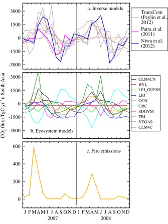
3.7 Seasonal variability of CO2fluxes

Figure 3 shows the comparisons of carbon fluxes as estimated by the terrestrial

ecosystem models (NEP), atmospheric-CO₂inverse models (NBP) and fire emissions

as estimated from satellite products and modeling. According to the ecosystem and

inversion models, the peak carbon release is around April–May, while the peak of CO2

5

uptake is between July and October. The dynamics as seen by the TransCom (global) inversion models is quite unconstrained due to the lack of atmospheric measurements

in the region. A recent study (Patra et al., 2011a) shows that the peak CO2 uptake

rather occurs in the month of August when inversion is constrained by regional mea-surements from commercial aircrafts. The months of peak carbon uptake are consis-10

tent with regional climate seasonality, i.e., the observed maximum rainfall during June– August months. This predominantly tropical biosphere is likely to be limited by water availability as the average daytime temperatures over this region are always above 20◦C and rainfall is very seasonal.

The peak-to-trough seasonal cycle amplitudes of NEP simulated by the ecosystem 15

models are of similar magnitude (∼300 Tg C yr−1) compared to those estimated by one of the inversion constrained by aircraft data (Patra et al., 2011a). The other regional inversion using atmospheric observations within the region estimated a seasonal cycle

amplitude about 50 % greater, mainly due to large CO₂ release in the months of May

and June (Niwa et al., 2012). A denser observational data network and field studies 20

are required for narrowing the gaps between different source/sink estimations.

3.8 Interannual variability of carbon fluxes

Because aircraft CO₂observations over South Asia region are limited to only two years (2007 and 2008), we will exclude inverse model estimates from the discussions on interannual variability.

25

(19)

BGD

9, 13537–13580, 2012

P. K. Patra et al.

Title Page

Tables Figures

◭ ◮

Back Close

Full Screen / Esc

Discussion

P

a

per

|

Dis

cussion

P

a

per

|

Discussion

P

a

per

|

Discussio

n

P

a

per

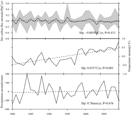
over South Asia from 1980 to 2009 (Fig. 4). The estimated net carbon flux (simula-tion scenario S2) over South Asia exhibits relatively large year-to-year change among the two simulation scenarios. The interannual variation of the 30-yr net carbon flux

estimated by the average of the ten models is 63 Tg C yr−1 measured by standard

de-viation, or 30 % measured by coefficient of variation (CV). In fact, the CV of the 30-yr 5

net carbon flux estimated by different models show a large range from 14 % to 166 %, and only two models show a CV of larger than 100 %.

The model ensemble unanimously show that interannual variations in simulated net carbon flux is driven by the interannual variability in gross primary productivity (GPP) rather than that in terrestrial heterotrophic respiration (H_R_{), suggesting that variations} 10

in vegetation productivity play a key role in regulating variations of the net carbon flux. Similar results were also found in other regions such as Africa (Ciais et al., 2009).

To study the effect of climate change on net carbon flux variations, we performed

correlation analyses between detrended anomalies of the modeled net carbon flux and detrended anomalies of climate (annual temperature and annual precipitation) over 15

the last three decades (see Methods section). All models predict that carbon uptake decrease or reversed into net carbon source responding to increasing temperature, with two models (LPJ GUESS and VEGAS) showing this positive correlation between temperature and net carbon flux statistically significant (r >_0.4, P <_{0.05). Regarding} the response to precipitation change, eight of the ten models predict more carbon 20

uptake in wetter years, particularly for LPJ; TRIFFID shows a statistically significant (P <_{0.05) negative correlation between precipitation and net carbon flux. Thus, warm} and dry years, such as 1988 and 2002, tend to have positive net carbon flux anomalies (less carbon uptake or net carbon release). This further implies that the warming trend and the and non-significant trend in precipitation (Fig. 4) during the last three decades 25

(20)

BGD

9, 13537–13580, 2012

P. K. Patra et al.

Title Page

Tables Figures

◭ ◮

Back Close

Full Screen / Esc

Discussion

P

a

per

|

Dis

cussion

P

a

per

|

Discussion

P

a

per

|

Discussio

n

P

a

per

|

variability in precipitation rather than in temperature. The precipitation is also found to be the main driver of seasonal variation in South Asian CO₂flux (Patra et al., 2011a).

3.9 Methane emissions

3.9.1 Top-down and bottom-up South Asian CH4emissions

The South Asian CH4 emissions are calculated from 6 scenarios prepared for the

5

TransCom-CH4 experiment (Patra et al., 2011b). Five of the emission scenarios are

constructed by combining inventories of various anthropogenic/natural emissions and wetland emission simulated by terrestrial ecosystem model (bottom-up), and one is

from atmospheric-CH4 inversion (top-down). The estimated CH4 emissions are in the

range of 33.2 and 43.7 Tg C-CH4yr−

1

for the period of 2000–2009, with an average 10

value of 37.2±3.7 (1σof 6 emission scenarios) Tg C-CH₄yr−1.

3.9.2 Bottom-up CH4 emissions from agriculture in India – implications for

South Asian budget

Livestock production and rice crop cultivation are the two major sources of CH4 emis-sion from the agriculture sector. The reported emisemis-sions due to enteric fermentation 15

and rice cultivation were 6.6 Tg C-CH4yr− 1

and 3.1 Tg C-CH4yr− 1

, respectively, using emission factors appropriate for the region (NATCOM, 2004). India is a major rice-growing country with a very diverse rice rice-growing environment: continuously or inter-mittently flooded, with or without drainage, irrigated or rain fed and drought prone. The average emission coefficient derived from all categories weighted for the Indian rice 20

crop is 74.1±43.3 kg C-CH4ha− 1

(Manjunath et al., 2011). The total mean emission (revised estimate) from the rice lands of India was estimated at 2.5 Tg C-CH₄yr−1_{. The} wet season contributes about 2.3 Tg C-CH4yr−

1

amounting to 88 % of the emissions. The emissions from drought-prone and flood-prone regions are 42 % and 18 % of the wet season emissions, respectively.

(21)

BGD

9, 13537–13580, 2012

P. K. Patra et al.

Title Page

Tables Figures

◭ ◮

Back Close

Full Screen / Esc

Discussion

P

a

per

|

Dis

cussion

P

a

per

|

Discussion

P

a

per

|

Discussio

n

P

a

per

India has the world’s largest total livestock population with 485 million in 2003, which

accounts for ∼57 % and 16 % of the world’s buffalo and cattle populations,

respec-tively. Methane emissions from livestock have two components: emission from

“en-teric fermentation” and “manure management”. Results showed that the total CH4

emission from Indian livestock, including enteric fermentation and manure manage-5

ment, was 11.8 Tg CH4 for the year 2003. Enteric fermentation itself accounts for

8.0 Tg C-CH4yr− 1

(∼91 %). Dairy buffalo and indigenous dairy cattle together

con-tribute 60 % of the total CH4 emission. The three states with high live stock CH4

emission are Uttar Pradesh (14.9 %), Rajasthan (9.1 %) and Madhya Pradesh (8.5 %).

The average CH4 flux from Indian livestock was estimated at 55.8 kg C-CH4ha−

1 10

feed/fodder area (Chhabra et al., 2009). The milching livestock constituting 21.3 % of the total livestock contribute 2.4 Tg C-CH₄yr−1

of emission. Thus, the CH₄emission per

kg milk produced amounts to 26.9 g C-CH4kg−

1

milk (Chhabra et al., 2009b). These CH4emission estimations of 8.8 Tg C yr−

1

from livestocks are in good

agree-ment with those of 8.8 (enteric feragree-mentation+manure management) Tg C yr−1 in the

15

Regional Emission inventory in Asia (REAS) for the year 2000 (Yamaji et al., 2003; Ohara et al., 2007), while emissions from rice cultivation of 2.5 Tg C yr−1is about half of 4.6 Tg C yr−1, estimated by Yan et al. (2009).

The REAS estimated total CH₄emissions due to anthropogenic sources (waste

man-agement and combustion, rice cultivation, livestock) from South Asia is 25 Tg C yr−1 for 20

the year 2000, with 6.5, 11.3 and 7.2 Tg C yr−1are emitted due to rice cultivation, live-stock and waste management. To match the range of the total flux from South Asia suggested by bottom-up inventories and atmospheric inversions (33.2–43.7 TgC/yr),

the remaining CH4sources (mostly natural wetlands and biomass burning) for

balanc-ing total emissions from South Asia is in the range of 8–19 TgC yr−1. The combination 25

of bottom-up estimations of all CH₄ sources types from all the member nations with

(22)

BGD

9, 13537–13580, 2012

P. K. Patra et al.

Title Page

Tables Figures

◭ ◮

Back Close

Full Screen / Esc

Discussion

P

a

per

|

Dis

cussion

P

a

per

|

Discussion

P

a

per

|

Discussio

n

P

a

per

|

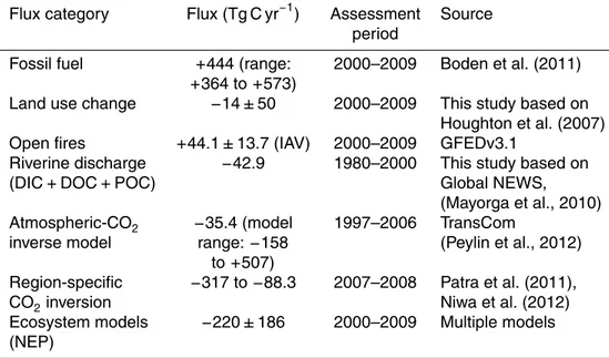
3.10 The carbon budget

3.10.1 Mean annual CO2budget

Figure 5 and Table 5 show the estimates of regional total CO₂-carbon emissions from

different source types as discussed above. A fraction of the CO2 emissions from fos-sil fuel burning (444 Tg C yr−1, averaged over 2000–2009) is taken up by the ecosys-5

tem within the region as suggested by the net biome productivity (NBP) estimated at −191±193 Tg C yr−1by bottom-up methods, and at−104±150 Tg C yr−1estimated by top-down methods. The bottom-up NBP is estimated as the sum of terrestrial ecosys-tem simulated net ecosysecosys-tem production (NEP), uptake and emissions due to land use

change (LUC), and carbon export through the river system. The estimated CO₂release

10

due to fires (44 Tg C yr−1) is of similar magnitude than the flux transported out of the land to the coastal oceans by riverine discharge (42.9 Tg C yr−1), but fire emissions are not included in the budget because are largely taken into account in the LUC compo-nent. Considering the net balance of these source types (including all biospheric and fossil fuel fluxes of CO2), the South Asia subcontinent is a net source of CO2, with 15

a magnitude in the range of 340 (top-down) to 253 (bottom-up) Tg C yr−1in the period

2000–2009. We choose the mean value of 297±244 Tg C yr−1from the two estimates

as our best estimate for the net land-to-atmosphere CO2flux for the South Asia region.

3.10.2 The mean annual carbon (CO2+CH₄) budget

Table 6 shows the emission and sinks of CO2 and CH4 for the South Asia region.

20

The best estimate of the total carbon or CO₂-equivalent (CO₂-eq₌CO₂₊CH₄) flux is 334 Tg C yr−1, calculated with the average CH4 emissions of 37 Tg C yr−

1

and best estimate of CO2emissions of 297 Tg C yr−

1

. For this CO2-eq flux, we assumed all CH4 is oxidized to CO2in the atmosphere within about 10 yr (Patra et al., 2011b). However,

it is well known that CH₄ exerts 23 times more radiative forcing (RF) than CO₂ over

25

(23)

BGD

9, 13537–13580, 2012

P. K. Patra et al.

Title Page

Tables Figures

◭ ◮

Back Close

Full Screen / Esc

Discussion

P

a

per

|

Dis

cussion

P

a

per

|

Discussion

P

a

per

|

Discussio

n

P

a

per

the region contributes RF-weighted CO2-eq emission of 1148 (297+37×23) Tg C yr− 1

. The net RF-weight CH4emission from the South Asia region is more than double of that released as CO₂from fossil fuel emissions. This result suggests that mitigation of CH₄ emission should be given high priority for policy implementation. The effectiveness of

CH4 emission mitigation is also greater due to shorter atmospheric lifetime compared

5

to CO₂.

4 Future research directions

The top-down and bottom-up estimations of carbon fluxes showed good agreements within their respective uncertainties, because we are able to account for the major flow of carbon in to and out of the South Asia regions. However, there are clearly some 10

missing flux components those require immediate attention. The fluxes estimated and not estimated in this work are schematically depicted in Fig. 6. Most notably the soil carbon pool and fluxes have not been incorporated in this analysis. The soil organic carbon (SOC) sequestration potential of the South Asia region is estimated to be in the range of 25 to 50 Tg C yr−1_{by restoring degraded soil and changing cropland} manage-15

ment practices (Lal, 2004). The carbon fluxes associated with international trade (e.g. wood and food products) are likely to be minor contributor to the total budget of South Asia, as the region is not a major exporter/importer of these products (FRA, 2010). The region is a major importer of coal and gas for supporting the energy supply (UN, 2010). These flux components, along with several others identified in Fig. 6, will be addressed 20

(24)

BGD

9, 13537–13580, 2012

P. K. Patra et al.

Title Page

Tables Figures

◭ ◮

Back Close

Full Screen / Esc

Discussion

P

a

per

|

Dis

cussion

P

a

per

|

Discussion

P

a

per

|

Discussio

n

P

a

per

|

5 Conclusions

We have estimated all major natural and anthropogenic carbon (CO2and CH4) sources

and sinks in the South Asia region using bottom-up and top-down methodologies. Excluding fossil fuel emissions and by accounting for the riverine carbon export, we

estimated a top-down CO2 sink for the 2000s (equal to the Net Biome Productivity)

5

of−104±150 Tg C yr−1based on recent inverse model simulations using aircraft mea-surement and median of multi-model estimate. The flux is in fairly good agreement with the bottom-up CO2flux estimate of −191±186 Tg C yr−

1

based on the net balance of the following fluxes: net ecosystem productivity, land use change, fire, and river ex-port. These results show the existence of a globally modest biospheric sink, but a quite 10

significant regionally and per area sink driven by the net growth and expansion of

veg-etation. In a longer time frame, the South Asia sink is also benefiting from the CO2

fertilization effect on vegetation growth.

Including fossil fuel emissions, our best estimate of the net CO2land-to-atmosphere flux is a source of 297±244 Tg C yr−1from the average of top-down and bottom-up esti-15

mates, and a net CO₂-equivalent, including both CO₂and CH₄, land-to-atmosphere flux of 334 Tg C yr−1 _{for the 2000s. We calculate that the RF-weighted total CH}

4 emission

is 851 Tg C yr−1 from the South Asia region. In terms of CO2-equivalent flux, methane is largely dominating the budget, at a 100-yr horizon, because of its larger warming potential compared to CO₂. This indicates that a mitigation policy for CH₄ emission is 20

preferred over fossil fuel CO2emission control or carbon sequestration in forested land. Further constraints in the carbon budget of South Asia to reduce current differences between the bottom-up and top-down estimates will require the expansion of atmo-spheric observations including key isotopes of greenhouse gases and the continuous development of inverse modeling systems that can use a diverse set of data streams 25

(25)

BGD

9, 13537–13580, 2012

P. K. Patra et al.

Title Page

Tables Figures

◭ ◮

Back Close

Full Screen / Esc

Discussion

P

a

per

|

Dis

cussion

P

a

per

|

Discussion

P

a

per

|

Discussio

n

P

a

per

constrain the role of wetlands in the methane budget, and expand observations on riverine carbon transport and its ultimate fate in the coastal and open oceans.

Acknowledgements. This work is a contribution to the REgional Carbon Cycle Assessment and Processes (RECCAP), an activity of the Global Carbon Project. The work is partly supported by JSPS/MEXT (Japan) KAKENHI-A (grant#22241008) and Asia Pacific Network 5

(grant#ARCP2011-11NMY-Patra/Canadell). Canadell is supported by the Australian Climate Change Science Program of CSIRO-BOM-DCCEE. The inverse model results of atmospheric

CO₂ and terrestrial ecosystem model results are provided under TransCom (http://transcom.

lsce.ipsl.fr) and TENDY (http://www-lscedods.cea.fr/invsat/RECCAP) projects, respectively, and we appreciate all the modelers’ contribution by providing access to their databases. 10

References

Acharyya, T., Sarma, V. V. S. S., Sridevi, B., Venkataramana, V., Bharti, M. D., Naidu, S. A., Kumar, B. S. K., Prasad, V. R., Bandopadhaya, D., Reddy, N. P. C., and Kumar, M. D.: Re-duced river discharge intensify phytoplankton bloom in Godavari estuary, India, Mar. Chem., 132–133, 15–22, 2012.

15

ALGAS (Asian Lest-Cost Greenhouse Gas Abettment Strategy): Report vol. 4, Asian Develop-ment Bank, Manila, 1998.

Aufdenkampe, A. K., Mayorga, E., Raymond, P. A., Melack, J. M., Doney, S. C., Alin, S. R., Aalto, R. E., and Yoo, K.: Riverine coupling of biogeochemical cycles between land, oceans, and atmosphere, Front. Ecol. Environ., 9, 53–60, 2011.

20

Awasthi, A., Uniyal, S. K., Rawat, G. S., and Rajvanshi, A.: Forest resource availability and its use by the migratory villages of Uttarkashi, Garhwal Himalaya (India), Forest Ecol. Manag., 174, 13–24, 2003.

Battin, T. J., Luyssaert, S., Kaplan, L. A., Aufdenkampe, A. K., Richter, A., and Tranvik, L. J.: The boundless carbon cycle, Nat. Geosci., 2, 598–600, 2009.

25

Bhattacharya, S. K., Borole, D. V., Francey, R. J., Allison, C. E., Steele, L. P., Krummel, P.,

Langenfelds, R., Masarie, K. A., Tiwari, Y. K., and Patra, P. K.: Trace gases and CO₂isotope

(26)

BGD

9, 13537–13580, 2012

P. K. Patra et al.

Title Page

Tables Figures

◭ ◮

Back Close

Full Screen / Esc

Discussion

P

a

per

|

Dis

cussion

P

a

per

|

Discussion

P

a

per

|

Discussio

n

P

a

per

|

Boden, T. A., Marland, G., and Andres, R. J.: Global, Regional, and National Fossil-Fuel CO₂

Emissions (1751–2008) Carbon Dioxide Information Analysis Center, Environmental Sci-ences Division, Oak Ridge National Laboratory, Oak Ridge, TN 37831–6290, USA, 2011. Bousquet, P., Ciais, P., Miller, J. B., Dlugokencky, E. J., Hauglustaine, D. A., Prigent, C., van

der Werf, G. R., Peylin, P., Brunke, E.-G., Carouge, C., Langenfelds, R. L., Lathi ´ere, J., 5

Papa, F., Ramonet, M., Schmidt, M., Steele, L. P., Tyler, S. C., and White, J.: Contribution of anthropogenic and natural sources to atmospheric methane variability, Nature, 443, 439– 443, 2006.

Bouwman, A. F., Boumans, L. J. M., and Batjes, N. H.: Modeling global annual

N₂O and NO emissions from fertilized fields, Global Biogeochem. Cy., 16, 1080,

10

doi:10.1029/2001GB001812, 2002.

Canadell J. G., Ciais, P., Gurney, K., Le Qu ´er ´e, C., Piao, S., Raupach M. R., and Sabine, C. L.:

An international e_ffort to quantify regional carbon fluxes, EOS, 92, 81–82, 2011.

Chhabra, A. and Dadhwal, V. K.: Assessment of pools and fluxes of carbon in Indian forests, Climatic Change, 64, 341–360, 2004.

15

Chhabra, A., Palria, S., and Dadhwal, V. K.: Spatial distribution of phytomass carbon in Indian forests, Global Change Biol., 8, 1230–1239, 2002.

Chhabra, A., Manjunath, K. R., Panigrahy, S., and Parihar, J. S.: Spatial pattern of methane emissions from Indian livestock, Current Sci., 96, 683–689, 2009a.

Chhabra, A., Manjunath, K. R., and Panigrahy, S.: Assessing the role of Indian livestock in cli-20

mate change, in: The International Archives of the Photogrammetry, Remote Sensing and Spatial Information Sciences, XXXVIII Part 8/W3, ISPRS WG VIII/6 – Agriculture, Ecosys-tem and Bio-diversity–Space Applications Centre (ISRO), Ahmedabad, India Indian Society of Remote Sensing, Ahmedabad Chapter, http://www.isprs.org/proceedings/XXXVIII/8-W3/, 359–365, 2009b.

25

Ciais, P., Piao, S.-L., Cadule, P., Friedlingstein, P., and Ch ´edin, A.: Variability and recent trends in the African terrestrial carbon balance, Biogeosciences, 6, 1935–1948, doi:10.5194/bg-6-1935-2009, 2009.

Cicerone, R. J. and Shetter, J. D.: Sources of atmospheric methane: measurements in rice paddies and a discussion, J. Geophys. Res., 86, 7203–7209, 1981.

30

(27)

BGD

9, 13537–13580, 2012

P. K. Patra et al.

Title Page

Tables Figures

◭ ◮

Back Close

Full Screen / Esc

Discussion

P

a

per

|

Dis

cussion

P

a

per

|

Discussion

P

a

per

|

Discussio

n

P

a

per

global carbon cycle: integrating inland waters into the terrestrial carbon budget, Ecosystems, 10, 172–185, 2007.

DeFries, R. S. and Townshend, J. R. G.: NDVI-derived land cover classification at global scales, Int. J. Remote Sens., 15, 3567–3586, 1994.

Emissions Database for Global Atmospheric Research (EDGAR), European Commission, Joint 5

Research Centre (JRC)/Netherlands Environmental Assessment Agency (PBL), release ver-sion 4.1, available at: http://edgar.jrc.ec.europa.eu, last access: 30 November 2010, 2010. Fekete, B. M., Wisser, D., Kroeze, C., Mayorga, E., Bouwman, A., Wollheim, W. M.,

and Vorosmarty, C. J.: Millennium ecosystem assessment scenario drivers (1970– 2050): climate and hydrological alterations, Global Biogeochem. Cy., 24, GB0A12, 10

doi:doi:10.1029/2009GB003593, 2010.

FRA: Global Forest Resource Assessment, Food and Agriculture Organization of the United Nations, Rome, 2010.

Fung, I., John, J., Lerner, J., Matthews, E., Prather, M., Steele, L. P., and Fraser, P. J.: Three-dimensional model synthesis of the global methane cycle, J. Geophys. Res., 96, 13033– 15

13065, 1991.

Galy, V., France-Lanord, C., Beyssac, O., Faure, P., Kudrass, H., and Palhol, F.: Efficient organic

carbon burial in the Bengal fan sustained by the Himalayan erosional system, Nature, 450, 407–410, 2007.

Goldewijk, K. K.: Estimating global land use change over the past 300 years: the HYDE 20

database, Global Biogeochem. Cy., 15, 417–433, 2001.

Hall, C. A. S. and Uhlig, J.: Refining estimates of carbon released from tropical land-use change, Can. J. Forest Res., 21, 118–131, 1991.

Haripriya, G. S.: Carbon budget of the Indian forest ecosystem, Climatic Change, 56, 291–319, 2003.

25

Hartmann, J., Jansen, N., D ¨urr, H. H., Kempe, S., and K ¨ohler, P.: Global CO₂consumption by

chemical weathering: what is the contribution of highly active weathering regions?, Global Planet. Change, 69, 185–194, 2009.

Houghton, R. A.: Revised estimates of the annual net flux of carbon to the atmosphere from changes in land use and land management 1850–2000, Tellus B, 55, 378–390, 2003. 30

(28)

BGD

9, 13537–13580, 2012

P. K. Patra et al.

Title Page

Tables Figures

◭ ◮

Back Close

Full Screen / Esc

Discussion

P

a

per

|

Dis

cussion

P

a

per

|

Discussion

P

a

per

|

Discussio

n

P

a

per

|

IPCC, Climate Change 2001: The Scientific Basis, Contribution of Working Group I to the Third Assessment Report of the Intergovernmental Panel on Climate Change, edited by: Houghton, J. T., Ding, Y., Griggs, D. J., Noguer, M., van der Linden, P. J., Da, X., Maskell, K., and Johnson, C. A., Cambridge Univ. Press, Cambridge, UK, 881 pp., 2001.

Ito, A. and Inatomi, M.: Use of a process-based model for assessing the methane budgets 5

of global terrestrial ecosystems and evaluation of uncertainty, Biogeosciences, 9, 759–773, doi:10.5194/bg-9-759-2012, 2012.

Kaul, M., Dadhwal, V. K., and Mohren, G. M. J.: Land use change and net C flux in Indian forests, Forest Ecol. Manag., 258, 100–108, 2009.

Kucharik, C. J., Foley, J. A., Delire, C., Fisher, V. A., Coe, M. T., Lenters, J. D., Young-Molling, C., 10

Ramankutty, N., Norman, J. M., and Gower, S. T.: Testing the performance of a dynamic global ecosystem model: water balance, carbon balance, and vegetation structure, Global Biogeochem. Cy., 14, 795–825, 2010.

Lal, R.: The potential of carbon sequstration in soils of South Asia, in: Conserving Soil and Water for Society: Sharing Solutions, 13th International Soil Conservation Organisation Con-15

ference, Brisbane, paper no. 134, 1–6, July 2004.

Lele, N. and Joshi, P. K.: Analyzing deforestation rates, spatial forest cover changes and iden-tifying critical areas of forest cover changes in North-East India during 1972–1999, Environ. Monit. Assess., 156, 159–170, 2009.

Machida, T., Matsueda, H., Sawa, Y., Nakagawa, Y., Hirotani, K., Kondo, N., Goto, K., 20

Nakazawa, T., Ishikawa, K., and Ogawa, T.: Worldwide measurements of atmospheric CO₂

and other trace gas species using commercial airlines, J. Atmos. Ocean. Tech., 25, 1744– 1754, 2008.

Manjunath, K. R., Panigrahy, S., Adhya, T. K., Beri, V., Rao, K. V., and Parihar, J. S.: Methane emission pattern of Indian rice-ecosystems, J. Ind. Soc. Remote Sens., 39, 307–313, 2011. 25

Marland, G. and Rotty, R. M.: Carbon dioxide emissions from fossil fuels: a procedure for esti-mation and results for 1950–82, Tellus B, 36, 232–261, 1984.

Matthews, E. and Fung, I.: Methane emissions from natural wetlands: global distribution, area, and ecology of sources, Global Biogeochem. Cy., 1, 61–86, doi:10.1029/GB001i001p00061, 1987.

30