Enhancing the representation of subgrid land surface characteristics in land surface models

(1)

GMDD

6, 2177–2212, 2013

Enhancing the subgrid land surface

representation in land surface models

Y. Ke et al.

Title Page

Abstract Introduction

Conclusions References

Tables Figures

◭ ◮

Back Close

Full Screen / Esc

Printer-friendly Version

Interactive Discussion

Discussion

P

a

per

|

Dis

cussion

P

a

per

|

Discussion

P

a

per

|

Discussio

n

P

a

per

|

Geosci. Model Dev. Discuss., 6, 2177–2212, 2013 www.geosci-model-dev-discuss.net/6/2177/2013/ doi:10.5194/gmdd-6-2177-2013

Geoscientiic Geoscientiic

Geoscientiic

Open Access

Geoscientiic

Model Development

Discussions

This discussion paper is/has been under review for the journal Geoscientific Model Development (GMD). Please refer to the corresponding final paper in GMD if available.

Enhancing the representation of subgrid

land surface characteristics in land

surface models

Y. Ke1,2, L. R. Leung2, M. Huang2, and H. Li2

1

Base of the State Key Laboratory of Urban Environment Process and Digital Modelling, Department of Resource Environment and Tourism, Capital Normal University,

105 Xi San Huan Bei Lu, Beijing, 100048, China

2

Pacific Northwest National Laboratory, 902 Battelle Boulevard, Richland, Washington, WA 99352, USA

Received: 6 February 2013 – Accepted: 12 March 2013 – Published: 28 March 2013

Correspondence to: L. R. Leung (ruby.leung@pnnl.gov)

(2)

GMDD

6, 2177–2212, 2013

Y. Ke et al.

Title Page

Tables Figures

◭ ◮

Back Close

Full Screen / Esc

Discussion

P

a

per

|

Dis

cussion

P

a

per

|

Discussion

P

a

per

|

Discussio

n

P

a

per

|

Abstract

Land surface heterogeneity has long been recognized as important to represent in the land surface models. In most existing land surface models, the spatial variability of sur-face cover is represented as subgrid composition of multiple sursur-face cover types. In this study, we developed a new subgrid classification method (SGC) that accounts for the 5

topographic variability of the vegetation cover. Each model grid cell was represented with a number of elevation classes and each elevation class was further described by a number of vegetation types. The numbers of elevation classes and vegetation types were variable and optimized for each model grid so that the spatial variability of both elevation and vegetation can be reasonably explained given a pre-determined 10

total number of classes. The subgrid structure of the Community Land Model (CLM) was used as an example to illustrate the newly developed method in this study. With similar computational burden as the current subgrid vegetation representation in CLM, the new method is able to explain at least 80 % of the total subgrid Plant Functional Types (PFTs) and greatly reduced the variations of elevation within each subgrid class 15

compared to the baseline method where a single elevation class is assigned to each subgrid PFT. The new method was also evaluated against two other subgrid methods (SGC1 and SGC2) that assigned fixed numbers of elevation and vegetation classes for

each model grid with different perspectives of surface cover classification. Implemented

at five model resolutions (0.1◦, 0.25◦, 0.5◦, 1.0◦and 2.0◦) with three maximum-allowed

20

total number of classesN class of 24, 18 and 12 representing different computational

burdens over the North America (NA) continent, the new method showed variable per-formances compared to the SGC1 and SGC2 methods. However, the advantage of the SGC method over the other two methods clearly emerged at coarser model

res-olutions and with moderate computational intensity (N class=18) as it explained the

25

most PFTs and elevation variability among the three subgrid methods. Spatially, the SGC method explained more elevation variability in topography-complex areas and more vegetation variability in flat areas. Furthermore, the variability of both elevation

(3)

GMDD

6, 2177–2212, 2013

Y. Ke et al.

Title Page

Tables Figures

◭ ◮

Back Close

Full Screen / Esc

Discussion

P

a

per

|

Dis

cussion

P

a

per

|

Discussion

P

a

per

|

Discussio

n

P

a

per

|

and vegetation explained by the new method was more spatially homogeneous re-gardless of the model resolutions and computational burdens. The SGC method will be implemented in CLM over the NA continent to assess its impacts on simulating land surface processes.

1 Introduction

5

As the terrestrial component of earth system models, land surface models play im-portant roles in representing the interactions between terrestrial biosphere and atmo-sphere, which is important for predicting future states of the earth system and assess-ing anthropogenic impacts on the climate system. Usassess-ing land surface parameters and meteorological forcing data as input, land surface models simulate key land processes 10

such as photosynthesis, respiration, and evapotranspiration that regulate mass, en-ergy, moisture, and momentum exchanges between soil, vegetation and atmosphere. Because terrestrial processes are sensitive to environmental drivers, realistic represen-tation of land surface characteristics is important for accurate estimation of surface heat

fluxes, terrestrial water storages and surface CO2 exchange required by atmospheric

15

models. Biases in land surface representation can lead to incorrect surface water and energy partitioning, and hence, inaccurate predictions of earth system change.

As a prominent feature of the landscape, land surface heterogeneity has long been recognized as important to represent, and has increasingly been incorporated in land surface models. It has been well established that subgrid spatial variability in land sur-20

face characteristics such as vegetation cover, soil moisture, and topography can

sig-nificantly affect the estimation of surface evapotranspiration, runoff, surface albedo,

snowpack, and other fluxes (Koster and Suarez, 1992; Seth et al., 1994; Ghan et al., 1997; Giorgi and Avissar, 1997; Giorgi et al., 2003; Li and Arora, 2012; Li et al., 2013). For example, Seth et al. (1994) reported that incorporation of subgrid scale in-25

homogeneity in land surface and climate forcing in the Biosphere-Atmosphere Transfer

(4)

GMDD

6, 2177–2212, 2013

Y. Ke et al.

Title Page

Tables Figures

◭ ◮

Back Close

Full Screen / Esc

Discussion

P

a

per

|

Dis

cussion

P

a

per

|

Discussion

P

a

per

|

Discussio

n

P

a

per

|

compared to homogeneous representation of land surface. Oleson et al. (2000) and Bonan et al. (2002a, b) found that replacing a single biome representation with plant functional types (PFTs) composition within each model grid cell caused considerable change in ground temperature, evaporation and albedo.

Among the land surface parameters, vegetation plays a key role in land-surface wa-5

ter and energy partitioning and carbon cycle. An accurate representation of vegetation distribution and properties is important in determining the spatial patterns of energy fluxes and biogeochemical cycling. Current land surface models widely adopt the con-cept of PFT to describe vegetation distributions (Oleson and Bonan, 2000; Krinner et al., 2005, Ek et al., 2003; Sitch, et al., 2003; Niu et al., 2011). For example, the Noah 10

land surface model incorporates 13 PFTs (Ek et al., 2003), CLM has 15 PFTs (Oleson et al., 2010), and ORCHIDEE distinguishes 12 PFTs (Krinner et al., 2012). While some models such as Noah represent a single dominant PFT in each model grid, models such as CLM represents subgrid spatial heterogeneity of vegetation distribution with a composition of multiple PFTs coexisting within each model grid. This representation 15

mainly focused on the fractional coverage of each PFT and assumes that all plants of the same type cluster as a “tile” within a model grid. The location of the PFTs, however, has seldom been explicitly described (Niu et al., 2011).

In addition to horizontal landscape variability, spatial heterogeneity in topography is also a pronounced land surface characteristic and has been considered in some land 20

surface simulations to help parameterize topographic variability in precipitation, tem-perature and snow processes (Leung and Ghan, 1995; Nijssen et al., 2001; Giorgi

et al., 203). Topography also a_ffects vegetation distribution especially on scales less

than 100 km (Leung and Ghan, 1998; Vankat, 1982; Barbour et al., 1987; Brown, 1994).

When combined, topography and vegetation have coupled effects on surface water and

25

energy fluxes. However, conventional subgrid methods usually considered only one parameter, i.e. either vegetation or topography distribution. Leung and Ghan (1995, 1998) developed a subgrid parameterization to incorporate the influence of topogra-phy on precipitation and snow cover and reported improved simulations in a regional

(5)

GMDD

6, 2177–2212, 2013

Y. Ke et al.

Title Page

Tables Figures

◭ ◮

Back Close

Full Screen / Esc

Discussion

P

a

per

|

Dis

cussion

P

a

per

|

Discussion

P

a

per

|

Discussio

n

P

a

per

|

climate model that used the subgrid parameterization with an explicit grid resolution of 90 km compared to simulations performed at a finer resolution of 30 km but without the subgrid parameterization. The method facilitated coupling with a distributed hydro-logic model for hydrohydro-logic simulations at the watershed scale (Leung et al., 1996), and was also found to perform well in global simulations (Ghan et al., 2006). The subgrid 5

parameterization of Leung and Ghan (1998) is one of few that incorporate the joint dis-tribution of both parameters. Taking advantage of the relationship between topography and vegetation, their method classifies the topography within each model grid into sub-grid elevation bands and parameterizes subsub-grid vegetation variability by considering vegetation distribution in each elevation band. Although only one dominant vegetation 10

type for each elevation class was considered because of the computation limit, this approach resulted in improved surface temperature simulation.

This study generalizes the method of Leung and Ghan (1998) and aims to develop

an improved and efficient subgrid scheme based on high-resolution satellite-based land

cover and topography products in order to enhance the representation of both vegeta-15

tion cover and topography. We chose the subgrid structure of CLM as an example and used the plant functional types defined in CLM to represent vegetation. CLM is a land model within the Community Earth System Model (CESM), formerly known as Com-munity Climate System Model (CCSM). It was designed for coupling with atmospheric models such as Community Atmosphere Model (CAM) and has been widely applied 20

at continental to global scales to understand the impact of land processes on climate change (Oleson et al., 2010).

The spatial heterogeneity of land surface parameters in CLM is represented using

a nested subgrid hierarchy. Each grid cell is composed of a di_fferent number of land

units including glacier, lake, wetland, urban and vegetated surfaces. Vegetated sur-25

faces are represented with composition of 15 possible Plant Functional Types (PFTs) such as Temperate Needleleaf Evergreen trees, Temperate Broadleaf Evergreen trees, etc., plus bare ground. In the current version of CLM (CLM 4.0), the PFT data is

(6)

GMDD

6, 2177–2212, 2013

Y. Ke et al.

Title Page

Tables Figures

◭ ◮

Back Close

Full Screen / Esc

Discussion

P

a

per

|

Dis

cussion

P

a

per

|

Discussion

P

a

per

|

Discussio

n

P

a

per

|

Ke et al., 2012) and the spatial distribution of each PFT within a model grid is not explicitly represented.

In this study, we developed a new subgrid PFT scheme in which the subgrid topo-graphic distribution of PFTs was described for each model grid. This requires classifi-cation of both vegetation types and elevation. The combined classificlassifi-cation of subgrid 5

topography and vegetation types can be computationally intensive in terrain-complex and species-rich area because a considerable number of elevation classes are needed to represent the diverse topographic relief while multiple vegetation types are required to explain a reasonable amount of vegetation variability. The method developed in this study assigned a flexible number of elevation bands and PFTs for each model grid and 10

optimized to explain a maximal amount of elevation and vegetation variations in a

com-putationally efficient manner. The method is applied to North America (NA) at different

model resolutions and evaluated by comparing it with other subgrid methods that use a fixed number of subgrid elevation bands and vegetation types.

2 Method

15

2.1 Plant Functional Types mapping

The PFT map for North America was generated at 500 m resolution based on the MODIS land cover product and climate data following the method presented in Ke et al. (2012). Briefly, seven PFTs including Needleleaf Evergreen trees, Needleleaf De-ciduous trees, Broadleaf Evergreen trees, Broadleaf DeDe-ciduous trees, shrub, grass and 20

crop were directly determined from the MODIS MCD12Q1 C5 PFT classifications for

each 500 m pixel. The WorldClim 5 arc-minute (0.0833◦) (Hijmans et al., 2005)

climato-logical global monthly surface air temperature and precipitation data was interpolated to the 500 m grids and the climate rules described by Bonan et al. (2002a) were used to reclassify the 7 PFTs into 15 PFTs in the tropical, temperate and boreal climate 25

groups. Similar to Lawrence and Chase (2007), the fractions of C3 and C4 grasses

(7)

GMDD

6, 2177–2212, 2013

Y. Ke et al.

Title Page

Tables Figures

◭ ◮

Back Close

Full Screen / Esc

Discussion

P

a

per

|

Dis

cussion

P

a

per

|

Discussion

P

a

per

|

Discussio

n

P

a

per

|

were mapped based on the method presented in Still et al. (2003). Pixels with bar-ren land and urban areas were reassigned to the bare soil class. Figure 1 shows the 500 m-resolution PFT map for NA.

2.2 Digital elevation model

The HYDRO1k digital elevation model (DEM) for NA was used to generate elevation 5

data. The HYDRO1k is a comprehensive and consistent geographic database provid-ing global coverage of topographically derived data sets such as elevation, slope, as-pect, flow accumulation raster layers, and stream lines vector layers. All raster data sets were generated from the USGS 30 arc-second global digital elevation model (GTOPO30) at 1 km resolution, and covered all global landmasses with the excep-10

tion of Antarctica and Greenland (http://eros.usgs.gov/). Compared to other existing global-scale elevation datasets such as the 90 m DEM of the Shuttle Radar Topogra-phy Mission (SRTM) (http://www2.jpl.nasa.gov/srtm/) and the Advanced Spaceborne Thermal Emission and Reflection Radiometer (ASTER) 30 m Global Digital Elevation Model (GDEM) (http://asterweb.jpl.nasa.gov/), HYDRO1k DEM has more complete 15

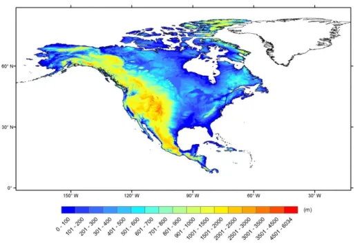
global coverage and its resolution is closer to existing global-scale land cover data such as the MODIS land cover product. Therefore, it has been widely used in conti-nental and global hydrologic and land surface modelling and was also selected in our study. For consistency with the PFT map, the elevation raster layer for North America was bilinearly interpolated to 500 m resolution (Fig. 2). We excluded Greenland from 20

our study because HYDRO1k does not cover this area.

2.3 Optimal Subgrid Classification (SGC) method of elevation and vegetation

The Subgrid Classification (SGC) method developed in our study considered the joint

distribution of elevation and vegetation. Within each model grid (e.g. at resolution 0.1◦×

0.1◦), the SGC method first classified surface elevation from the 500 m DEM data into

25

(8)

GMDD

6, 2177–2212, 2013

Y. Ke et al.

Title Page

Tables Figures

◭ ◮

Back Close

Full Screen / Esc

Discussion

P

a

per

|

Dis

cussion

P

a

per

|

Discussion

P

a

per

|

Discussio

n

P

a

per

|

area threshold of 1 % was used to limit the area of each elevation band. That is, an elevation band containing less than 1 % of the land area of the model grid is added to the neighboring elevation band so that each elevation band covers at least 1 % of the grid land area. Within each elevation band in each model grid, the area was further classified into a limited number of PFTs. For example, if the subgrid surface 5

elevation within a model grid was divided intoM elevation bands and the vegetation

within each elevation band was classified intoNPFTs, the model grid was represented

with a total number ofM×N subgrid classes, with each elevation-PFT class treated as

a computational unit in the land surface model.

To reduce computational burden, we set the maximum-allowed total number of sub-10

grid classes to “N class” (e.g. 18 classes) for each model grid. The number of

ele-vation bands M and the number of PFTs N for each elevation band are variable for

each model grid butM×N should not exceed the maximum-allowed numberN class

(e.g. 18). Hence the combination of M and N is variable and is chosen to best

rep-resent the subgrid variability of both PFT and elevation. For example, for a total of 18 15

maximum-allowed subgrid classes (N class=18), possible combinations include 3

el-evation bands and 6 PFTs per elel-evation band, or 2 elel-evation bands and 9 PFTs per elevation band, etc., but the optimal combination was selected. Two criteria must be satisfied for the optimal classification: (1) the elevation range of each elevation band is less than and close to 100 m; and (2) total percentage of subgrid PFTs correctly clas-20

sified by the method is no less than 80 % for each model grid. We prioritized criteria (2) so that if none of the combinations satisfies both conditions, the classification explain-ing more than 80 % of PFTs and with elevation range greater than but closest to 100 m was selected; if more than one combination satisfy both conditions, the classification that correctly classifies the most subgrid PFTs was selected.

25

2.4 SGC method evaluation

In CLM 4.0, vegetation was represented as the composition of 15 PFTs plus bare soil. The simplest and least computationally intensive way to incorporate elevation

(9)

GMDD

6, 2177–2212, 2013

Y. Ke et al.

Title Page

Tables Figures

◭ ◮

Back Close

Full Screen / Esc

Discussion

P

a

per

|

Dis

cussion

P

a

per

|

Discussion

P

a

per

|

Discussio

n

P

a

per

|

distribution of vegetation is to assign a single elevation band to each PFT within a model grid, that is, the surface elevation in the area covered by each PFT was aggregated to one elevation band. We used this method as a baseline to assess the performance of

the SGC method with similar computational burden at different model resolutions.

The SGC method was also evaluated by comparing it with two other subgrid clas-5

sification methods based on a fixed number of elevation bands and vegetation types.

The first subgrid classification method (SGC1) was the M elevation bands-N PFTs

method. Each model grid cell is first divided intoM equal-interval elevation bands and

each elevation band was further classified intoN PFTs. The second subgrid

classifica-tion method (SGC2) was theN PFTs-M elevation bandsmethod. Each model grid cell

10

was first classified intoN PFTs and the area covered by each PFT was further divided

intoM equal-interval elevation bands. For both methods, we used the minimum area

threshold of 1 % to restrict the number of elevation bands in the same way that was

used in the SGC method. The SGC1 and SGC2 methods take di_fferent perspectives

of topographic-vegetation distribution in that SGC1 examines the PFT distribution at 15

different elevation bands and SGC2 examines the elevation distribution of each PFT.

However, both methods classify the model grids into fixed numbers of elevation bands

and PFTs and the total number of classes isM×N per model grid throughout the study

area.

We implemented the classification methods SGC, SGC1 and SGC2 in North America 20

at 0.1◦, 0.25◦, 0.5◦, 1.0◦, and 2.0◦resolution with different combinations of number of

el-evation bands and vegetation types: (1)Scheme 1:N class=24,M₌6,N₌4,

mean-ing 24 maximum-allowed classes for the SGC method and the combination of 6

eleva-tion bands and 4 PFTs for the SGC1 and SGC2 methods; (2)Scheme 2:N class=18,

M₌6, N₌3; and (3) Scheme 3: N class=12, M₌4, N₌3. The baseline subgrid

25

method was also implemented at the five resolutions. The three schemes represent

different computational burdens with Scheme 1 being most computationally intensive

(10)

GMDD

6, 2177–2212, 2013

Y. Ke et al.

Title Page

Tables Figures

◭ ◮

Back Close

Full Screen / Esc

Discussion

P

a

per

|

Dis

cussion

P

a

per

|

Discussion

P

a

per

|

Discussio

n

P

a

per

|

Spatial and statistical comparisons of the three methods at different model

resolu-tions and with different vegetation/elevation combinations were performed in order to

compare their abilities to explain the joint distributions of both vegetation and elevation. Generally, the total percentage of PFTs explained within each model grid was used to measure the method’s ability to characterize subgrid vegetation; the mean standard 5

deviation of elevation averaged over all elevation bands σ_ep (Eqs. 1, 2) within each

model grid and the mean elevation interval for all elevation bandsI_ep (Eqs. 3, 4) were

used to measure how well the method describes the subgrid variability of topography.

For the SGC and SGC1 methods,σ_ep at a given model grid was calculated as:

σ_ep₌ 1 N_b

N_b X

i=1

σ_eb(i) (1)

10

whereσ_eb(i) is the standard deviation of subgrid surface elevation within thei-th

ele-vation band, andN_bis the number of elevation bands in that grid.

For the baseline and SGC2 methods,σ_ep was calculated as:

σ_ep₌ 1 N_P

N_P X

j=1



 1 N_b

N_b X

i=1

σ_eb(i,j) 

 (2)

where σ_eb(i,j) is the standard deviation of subgrid surface elevation within the i-th

15

elevation band for thej-th dominant PFT, andN_P is the number of dominant PFTs in

that grid. For the baseline method,N_Pcan be any number within 16 because all PFTs

within each model grid were included, andN_bequals to 1 because only one elevation

band was assigned to each PFT.

Similarly, for the SGC and SGC1 methods,I_ep at a given model grid was calculated

20 as:

I_ep₌ 1 N_b

N_b X

i=1

I_eb(i) (3)

(11)

GMDD

6, 2177–2212, 2013

Y. Ke et al.

Title Page

Tables Figures

◭ ◮

Back Close

Full Screen / Esc

Discussion

P

a

per

|

Dis

cussion

P

a

per

|

Discussion

P

a

per

|

Discussio

n

P

a

per

|

whereI_eb(i) is the elevation interval for thei-th elevation band, which is calculated as

the di_fference between the maximum and minimum elevation within thei-th elevation

band.

For the baseline and SGC2 methods,I_ep was calculated as:

I_ep₌ 1 N_P

N_P X

j=1



 1 N_b

Nb

X

i=1

I_eb(i,j) 

 (4)

5

whereI_eb(i,j) is the elevation interval within thei-th elevation band for thej-th PFT. In

the next section, the spatial distributions of the percentage of PFTs explained by the

method andσ_ep were visually examined; the average percentage of PFTs explained

and averageσ_ep andI_epacross NA and their standard deviations were also compared.

3 Results and discussions

10

3.1 The SGC method

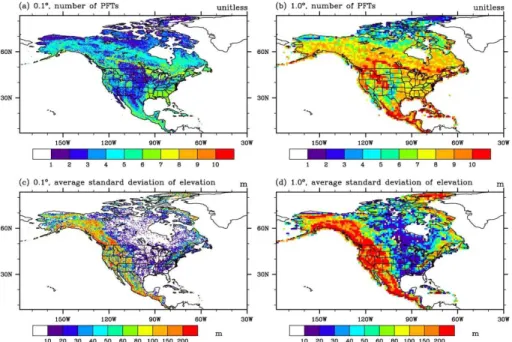
Figure 3 shows the number of PFTs and the average standard deviation of elevation

for all PFTs (σ_ep, Eq. 2) from the baseline subgrid classification method over the NA

continent at 0.1◦and 1.0◦resolutions. At both spatial resolutions, more PFT classes per

grid, i.e. greater subgrid variability of vegetation is found in the coastal areas (over 5 15

PFTs) than in the inland region such as the Great Plains (1–2 PFTs at 0.1◦resolution)

where crop dominates the landscape. Increasing model grid size results in greater subgrid-scale variability of PFTs (Fig. 3a, b). When assigning one elevation band to

each PFT within the model grid,σ_epshows substantial spatial variance across the

con-tinent (Fig. 3c, d). It is evident that the spatial distribution ofσ_epcorresponds with

topo-20

graphic variations. In western NA with complex topography such as the Coastal Range

and Rocky Mountains, σ_ep is larger than in flat areas such as the Great Plains and

(12)

GMDD

6, 2177–2212, 2013

Y. Ke et al.

Title Page

Tables Figures

◭ ◮

Back Close

Full Screen / Esc

Discussion

P

a

per

|

Dis

cussion

P

a

per

|

Discussion

P

a

per

|

Discussio

n

P

a

per

|

resolution as the subgrid topographic variability becomes larger. In the western NA,

σ_ep is above 200 m and reaches 1000 m, while σ_ep decreases to below 30 m in the

Great Plains at 1.0◦ resolution. The averageσ_epacross the continent rapidly increases

from 43.1 m at 0.1◦ resolution to 59.1 m at 0.25◦ resolution, 76.0 m at 0.5◦ resolution,

94.8 m at 1.0◦resolution, and 119.3 m at 2.0◦resolution, indicating that with the

base-5

line method, substantially less subgrid topographic details are represented at coarser resolution.

Compared to the baseline method where the number of PFTs and the number of el-evation band per PFT were pre-determined, the optimal SGC method produced much more spatially variant number of elevation bands and number of PFTs within each el-10

evation band throughout the continent (Figs. 4a, b, 5a, b, and 6a, b). With comparable

number of total classes (15 classes for the baseline method andN class=18 for the

SGC method), the SGC method substantially suppressesσ_epespecially in

topography-complex areas (Fig. 3c vs. Fig. 5d, Fig. 3d vs. Fig. 6d), indicating that greater detail of subgrid topography was described by the SGC method. The advantage of the SGC 15

method over the baseline method in explaining elevation variability is more prominent

at coarser resolution (Fig. 3d vs. Fig. 6d) as σ_ep is generally less than 60 m for the

SGC method in the Pacific Northwest (Fig. 6d) compared to over 200 m for the base-line method (Fig. 3d). However, more detailed elevation information in the SGC method compromises the representation of PFTs compared to the baseline method that con-20

siders all PFTs within each model grid. Nevertheless, the SGC method still explained a reasonable amount of PFT variability (over 80 % in Figs. 5c, 6c) while greatly im-proving the elevation variability, which has equally if not larger impacts on land surface processes as PFT variability (Leung and Ghan, 1998), at computational cost compara-ble to the baseline method.

25

The comparison between different N class (Figs. 4b, 5b) and varying model

reso-lutions (Figs. 5b, 6b) shows that both the number of elevation bands and number of PFTs demonstrate similar spatial pattern in North America. In the areas with more complex topography such as the Coastal Range, Rocky Mountains, and Appalachian

(13)

GMDD

6, 2177–2212, 2013

Y. Ke et al.

Title Page

Tables Figures

◭ ◮

Back Close

Full Screen / Esc

Discussion

P

a

per

|

Dis

cussion

P

a

per

|

Discussion

P

a

per

|

Discussio

n

P

a

per

|

Mountains (Fig. 2), the SGC method generated substantially more elevation bands than in flat areas such as the Central and Coastal Plains (Figs. 3b, 4b, 5b). The spa-tial distribution of the number of PFTs within each elevation band, on the other hand, generally shows an opposite pattern (Figs. 3a, 4a, 5a). In western NA where more el-evation bands were generated, smaller numbers of PFTs within each elel-evation bands 5

were produced because the combined number of PFTs and elevation bands was

re-stricted by N class. Still, the total PFTs explained by the method was over 80 % for

each model grid (Figs. 4c, 5c, 6c) because driven by climate, PFT is more correlated with elevation in over complex terrains. This allows the SGC method to optimally rep-resent subgrid variations in both topography and vegetation. In the flat areas of central 10

and eastern NA, more than six PFTs were generated that explained over 98 % of the total PFTs in the model grids. In the Great Plains, only one to two elevation bands and no more than two PFTs within each elevation band were generated for the flat terrain and cropland-dominated landscape.

To assess the impacts ofN class, we note from Figs. 4d and 5d that 24 total classes

15

reduced the mean standard deviations of elevation averaged from all elevation bands

in western NA compared to 18 total classes because finer elevation intervals a_fforded

by using a larger number of elevation bands yield more detailed representation of

topographic relief. However, decreasing N class does not considerably influence the

number of PFTs per elevation band (Figs. 4a, 5a) at 0.1◦ resolution. Reducing model

20

resolution from 0.1◦to 1.0◦ resulted in generally more elevation bands and more PFTs

per elevation band because the model grids encompass greater subgrid variability of vegetation and topography.

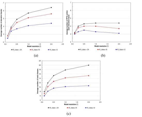
Figure 7 illustrates that the average number of elevation bands, number of PFTs per band, and the number of total classes generated by the SGC method show similar in-25

creasing trends with decreasing model resolutions and increasing number ofN class.

At the finest resolution of 0.1◦, the average number of total classes increases only

slightly with increasingN class (6 for N class of 12, 7 for N class of 18, and 7.9 for

(14)

GMDD

6, 2177–2212, 2013

Y. Ke et al.

Title Page

Tables Figures

◭ ◮

Back Close

Full Screen / Esc

Discussion

P

a

per

|

Dis

cussion

P

a

per

|

Discussion

P

a

per

|

Discussio

n

P

a

per

|

represented by a small number of subgrid classes. At resolution of 2◦, the average

number of total classes increases to 10.2, 15.2, and 20, for N class equals 12, 18,

and 24, respectively. As the subgrid topography and vegetation variation increase with coarser model resolution, more classes are required to explain a reasonable amount of topography and vegetation variations and the method is more restricted by the 5

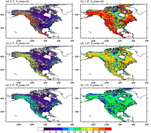
maximum-allowed number of classes. This is consistent with what can be seen in Fig. 8, which shows the spatial distribution of the actual number of classes generated

from the SGC method. At 0.1◦ model grid size, changing N class does not

signifi-cantly change the number of classes except in western NA with complex topogaphy.

At 1◦resolution, the number of classes decrease dramatically with decreasingN class

10

throughout the NA continent. There is no distinct difference between the flat areas

and the topographically-complex areas especially whenN class is 12. These show the

method’s ability in assigning optimal classes for different model resolutions and a larger

number of maximum-allowed total classes gives more flexibility in assigning the best suitable combination of elevation bands and PFTs.

15

Comparison of Fig. 7a and c indicates that the increase in the number of total classes is mainly attributed to the increase in the number of elevation bands as both metrics show similar trend. In contrast, the average number of PFTs per elevation band in-creases more slowly, and can even decrease with increasing model grid size. For

ex-ample, on average 3.3 PFTs are produced within each elevation band at 1◦resolution

20

(N class=12 in Fig. 7b), but only 3.1 PFTs are needed for each elevation band at 2◦

resolution (N class=12 in Fig. 7b) to explain at least 80 % of total PFTs. This

indi-cates that the subgrid variability of surface elevation changes more dramatically than the subgrid variability of vegetation type with changing model resolution and highlights the importance of considering the topographic distribution of vegetation types.

25

3.2 Comparison of three subgrid classification methods

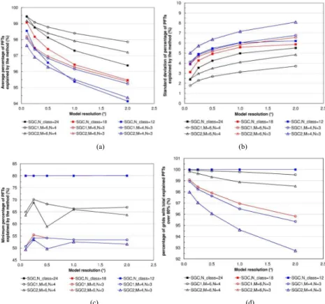
The optimal subgrid classification method SGC was evaluated against the SGC1 and SGC2 methods with fixed number of elevation bands and PFTs. Figure 9a shows that

(15)

GMDD

6, 2177–2212, 2013

Y. Ke et al.

Title Page

Tables Figures

◭ ◮

Back Close

Full Screen / Esc

Discussion

P

a

per

|

Dis

cussion

P

a

per

|

Discussion

P

a

per

|

Discussio

n

P

a

per

|

all three methods explained a large fraction of total PFTs above 94 %. The percentage of PFTs represented by each method, when averaged across the NA continent,

de-creases with increasing model grid size and decreasing number of elevation bandsM

or PFTsN (Fig. 9a). The standard deviation of the percentage PFTs explained across

the NA continent increases with increasing model grid size and decreasingM and N

5

(Fig. 9b). WithM₌6, N₌4 and N class=24, the SGC1 method, which first

classi-fies topography into 6 elevation bands and represents each elevation band with 4 most dominant PFTs explains the most PFTs, while the optimal classification method

pro-duced the lowest percentage of PFTs except at 0.1◦resolution.

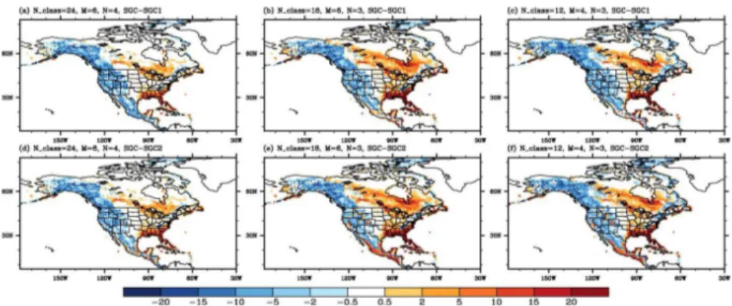
The spatial distribution of the differences in the percentage of PFT explained

10

(Fig. 10a, d) illustrates that areas with less PFTs explained by the SGC method (nega-tive values of SGC-SGC1 or SGC-SGC2) mainly concentrate in the mountainous west-ern NA with complex topography. The SGC method explains 2–15 % less PFTs than the other two methods. In these areas, the SGC method required more elevation bands to represent reasonable variations of elevation (e.g. over 10 elevation bands were pro-15

duced in these areas in Fig. 4b), thus sacrificing the total PFTs represented (only 2–3 PFTs were identified in this area in Fig. 4a compared to four PFTs used in SGC1 and SGC2 methods). Despite the lower amount of PFTs explained in the western NA, more PFTs are explained by the SGC method than the other two methods in the south-east United States such as Florida, Mississippi, South Carolina and Georgia, and in 20

central Canada where the SGC method identified more than four PFTs because few elevation classes are needed to represent the flat topography. When fewer PFTs were

used in SGC1 and SGC2 and fewerN class was used in SGC, the areas of positive

difference in the percentage of PFT explained between SGC and the other two

meth-ods expanded from central Canada to Alberta and Saskatchewan provinces in western 25

(16)

GMDD

6, 2177–2212, 2013

Y. Ke et al.

Title Page

Tables Figures

◭ ◮

Back Close

Full Screen / Esc

Discussion

P

a

per

|

Dis

cussion

P

a

per

|

Discussion

P

a

per

|

Discussio

n

P

a

per

|

With 18 maximum-allowed number of total classes in the SGC method,M=6 and

N₌3, the negative differences in PFTs between SGC and the other two methods were

compensated by positive differences (Fig. 10b, e). Hence overall, the average

percent-age of PFTs explained by SGC is higher than the other two methods across all

reso-lutions (Fig. 9a). AsN class decreases to 12, at the finest resolution of 0.1◦, SGC

ex-5

plained slightly greater percentage of PFTs than the other methods. With this computa-tional burden, as model grid size increases the performance of SGC decreases rapidly as indicated by the rapid decrease in the percentage PFTs explained (Fig. 9a) and

increase in the standard deviation of PFTs (Fig. 9b). At the resolution of 1◦ or higher,

SGC explained lower amount of PFTs than the other two methods. As stated above, at 10

coarse resolution SGC is more restricted by the number of maximum-allowed classes because larger variations of PFTs and topography exist. Since topography shows more distinct change than PFTs (Fig. 7a, b), the balance between the number of elevation bands and PFTs resulted in less PFTs explained by the method.

Although the SGC method shows varying performances in terms of the average 15

percent of PFTs explained compared to the other two methods, the PFTs explained by this method is more spatially homogeneous – all model grids in the study area

have over 80 % of total PFTs explained regardless ofN class and model resolution. In

contrast, the PFTs explained by SGC1 and SGC2 can be as low as 52 % (Fig. 9c), and around 92.7 % of the model grids have over 80 % of the PFTs explained (Fig. 9d). 20

The abilities of the three methods in explaining topographic variation were shown in

Fig. 11. For all three methods, the average standard deviation of elevationσ_epfor all

el-evation bands increase with model grid size. Sinceσ_epindicates the subgrid variation of

elevation within each elevation band, smaller value of averageσ_epmeans better overall

representation of subgrid topography, and vice versa. It is apparent that classifying the 25

surface elevation into a limited number of elevation bands greatly reduce the standard deviation of elevation represented in the model grids; for example, the average stan-dard deviation of elevation within the model grids varies from 59.1 m to 119.3 m from

(17)

GMDD

6, 2177–2212, 2013

Y. Ke et al.

Title Page

Tables Figures

◭ ◮

Back Close

Full Screen / Esc

Discussion

P

a

per

|

Dis

cussion

P

a

per

|

Discussion

P

a

per

|

Discussio

n

P

a

per

|

0.1◦ to 1◦ resolution for the baseline method, while the averageσ_ep substantially

de-creased and the ranges narrow down to 9.4 from 63.4 (Fig. 10a) for the SGC method.

At fine resolutions from 0.1◦ to 0.5◦, the average σ_ep from the SGC method with

N class of 24 (and 18) is greater than the SGC1 and SGC 2 methods withM₌6 and

N₌4 (andN₌3) (Fig. 11a), meaning that SGC1 and SGC2 have better overall

repre-5

sentation of elevation variability at these scales. When model resolution decreases, the

advantage of the SGC method in elevation representation emerges. At both 1◦and 2◦

resolutions, the averageσ_epfrom SGC is lower than that from SGC1 and SGC2.

Com-parison of the spatial distribution ofσ_ep in Fig. 12 shows that at both fine and coarse

resolutions, the SGC method produced distinctly lowerσ_ep in western NA and the

Ap-10

palachian Mountains region than the other two methods, as the number of elevation

bands in these areas increased (over 6 in Figs. 4b, 5b, 6b). Althoughσ_ep in flat areas

from SGC is slightly greater than that from the other two methods, SGC is still able

to produce reasonable representation of elevation variability as σ_ep is less than 30 m

in these areas (Figs. 3d, 4d, 5d). This implies that using 6 or 4 elevation bands may 15

be redundant in these areas because topography does not vary much and vegetation distribution has little relation to topography.

Compared to those from SGC1 and SGC2, the averageσ_ep from SGC climbs more

slowly with increasing model grid size and decreasing number of maximum-allowed

classes. For example, the averageσ_ep from SGC with 24 N class ranges from 16.2

20

to 30.2 across resolutions from 0.1◦ to 2◦, while SGC2 with 4 PFTs and 6 elevation

bands within each PFT-covered area produced averageσ_epfrom 9.4 to 38.6, and SGC1

produced even larger range of average σ_ep from 11.1 to 46.9. The average elevation

intervalI_ep shows similar pattern (Fig. 11c). Because topography shows much greater

variability at coarser scales, the slower change in average σ_ep indicates more stable

25

performance of the SGC method across different scales.

Although the averageσ_epfrom SGC is higher than that from the other methods at fine

resolution (e.g. less than 1◦), the variation ofσ_ep across NA is smaller than that from

(18)

GMDD

6, 2177–2212, 2013

Y. Ke et al.

Title Page

Tables Figures

◭ ◮

Back Close

Full Screen / Esc

Discussion

P

a

per

|

Dis

cussion

P

a

per

|

Discussion

P

a

per

|

Discussio

n

P

a

per

|

computational burden. This means that the elevation variability explained by the SGC method is more spatially homogeneous than the other two methods. The SGC method adjusts the number of elevation bands flexibly to ensure that the elevation range within each elevation band for each model grid is less than and close to 100 m at the premise of over 80 % PFTs explained in the model grid. Therefore more elevation bands were 5

produced in complex terrain than in flat land surface. In contrast, SGC1 and SGC2 represent the subgrid elevation in each model grid by a fixed number of elevation bands

regardless of the land surface topography. Hence they can produce very smallσ_epin flat

area but largeσ_epin mountainous regions. The spatial homogeneity of the SGC method

is also noted in Fig. 11d. At the same resolution and with the same computational 10

burden, there are more model grids with less than 100 m average elevation interval per elevation band from the SGC method than those from the other methods. For example, using the SGC method, over 80 % of the grid cells have less than 100 m elevation

range within the elevation bands even at 2◦ resolution (N class₌24), while with the

same computational burden the percentage of grids decreases to 54 % for SGC1 and 15

47 % for SGC2 (M=6,N₌4).

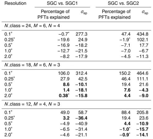
The combined examination of Figs. 9–12 and the statistical analysis in Table 1 show that the SGC method is not necessarily superior to the other two methods in terms of both vegetation and elevation variation explained, when a large number of subgrid

classes is allowed (N class₌24). However, when computational burden is moderately

20

alleviated using fewer number of subgrid classes (N class=18,M₌6 andN₌3), the

SGC method begins to demonstrate its advantage in balancing the variability of

vege-tation and elevation distribution that can be explained. At the coarser resolutions of 1◦

to 2◦, the SGC method becomes clearly superior to both SGC1 and SGC2, i.e. a

sta-tistically greater percentage of PFTs was explained and σ_ep is smaller. With N class

25

of 12, the SGC method is better than SGC2 at the resolutions of 0.5◦ or coarser and

better than SGC1 only at the resolution of 0.25◦.

(19)

GMDD

6, 2177–2212, 2013

Y. Ke et al.

Title Page

Tables Figures

◭ ◮

Back Close

Full Screen / Esc

Discussion

P

a

per

|

Dis

cussion

P

a

per

|

Discussion

P

a

per

|

Discussio

n

P

a

per

|

4 Conclusions

In this study we presented a new subgrid method to enhance the representation of land surface characteristics in land surface models. Built on the current subgrid structure of CLM that defines subgrid fractional area of multiple PFTs, the method incorporates topographic distributions of PFTs. For each model grid, the method assigned variable 5

elevation and vegetation classes based on their joint distribution so that the

subgrid-scale variability of both can be explained in an optimal and computationally efficient

manner. Compared to the baseline method, which assigns a single elevation class to each PFT, the new method provides an obvious advantage in representing topographic

variability at a similar computational e_fficiency as the average standard deviation of

sur-10

face elevation in each elevation band was greatly suppressed. Although this compro-mised the ability to represent vegetation variability compared to the baseline method, the new method still explained at least 80 % of the total PFTs in each model grid. The

effectiveness of the new method in representing subgrid variability in both topography

and vegetation is partly related to the correlation between topography and vegetation. 15

However, this e_ffectiveness decreases with decreasing model resolution because the

elevation dependence of vegetation is weaker at coarser spatial scales.

Compared to the other subgrid approaches with pre-determined number of eleva-tion classes and vegetaeleva-tion types (SGC1 and SGC2), the new method presented in this study assigned variable number of elevation and vegetation classes to balance 20

the representation of both topography and vegetation variability under the restriction of

a maximum-allowed number of total classes. Among the three schemes with di_fferent

computational burdens, the new method shows advantages over the other methods with moderate computation intensity and at coarse scales in that both PFTs and topog-raphy variability was best explained. Furthermore, the variability of both vegetation and 25

(20)

GMDD

6, 2177–2212, 2013

Y. Ke et al.

Title Page

Tables Figures

◭ ◮

Back Close

Full Screen / Esc

Discussion

P

a

per

|

Dis

cussion

P

a

per

|

Discussion

P

a

per

|

Discussio

n

P

a

per

|

Spatial heterogeneity of surface cover and topography has important control on many

land processes. This study assessed different methods to classify the subgrid spatial

distribution of surface cover and topography. When implemented in the model, the frac-tional area of each elevation band and PFT can be determined and the mean elevation of each elevation band can be defined. Separate calculations of surface processes 5

can be performed for each class, and the output fluxes at each class can then be aggregated in an area-weighted manner for each grid cell. To maximize the benefits of representing both subgrid PFT and topography on land surface and coupled land-atmosphere simulations, subgrid atmospheric forcings such as temperature, precipita-tion, and radiation should be provided to account for the important influence of topog-10

raphy on atmospheric processes. Subgrid parameterizations such as Leung and Ghan (1998) to represent the subgrid topographic influence on precipitation or simple lapse rate based adjustment of temperature and precipitation (e.g. Liang et al., 1994) should be explored. The impacts of the new subgrid classification on land surface simulations

at different model resolutions will be studied in the future.

15

Acknowledgements. The authors acknowledge the Pacific Northwest National Laboratory

(PNNL) Platform for Regional Integrated Modeling and Analysis (PRIMA) Initiative, which sup-ported the development of databases used in the study, and the Climate Science for Sustain-able Energy Future (CSSEF) project funded by the Department of Energy (DOE) Earth System Modeling program, which supported the development and analysis of various subgrid classi-20

fication methods. PNNL is operated by Battelle for the DOE under Contract DE-AC06-76RLO 1830. The first author also acknowledges the support from the Key Program of National Nat-ural Science Foundation of China (NSFC) (41130744/D0107), the General Program of NFSC (41171335/D010702), and the 973 Program of China (2012CB723403).

References

25

Barbour, M. G., Burk, J. H., and Pitts, W. D.: Terrestrial Plant Ecology, 3rd Edn., Ben-jamin/Cummings, Publishing Co., Menlo Park, California, 688 pp., 1998.

(21)

GMDD

6, 2177–2212, 2013

Y. Ke et al.

Title Page

Tables Figures

◭ ◮

Back Close

Full Screen / Esc

Discussion

P

a

per

|

Dis

cussion

P

a

per

|

Discussion

P

a

per

|

Discussio

n

P

a

per

|

Bonan, G. B., Levis, S., Kergoat, L., and Oleson, K. W.: Landscapes as patches of plant func-tional types: an integrating concept for climate and ecosystem models, Global Biogeochem. Cy., 16, 5-1–5-23, doi:10.1029/2000GB001360, 2002a.

Bonan, G. B., Oleson, K. W., Vertenstein, M., Levis, S., Zeng, X., Dai, Y., Dickinson, R. E., and Yang, Z. L.: The land surface climatology of the Community Land Model coupled 5

to the NCAR Community Climate Model, J. Climate, 15, 3123–3149, doi:10.1175/1520-0442(2002)015<3123:TLSCOT>2.0.CO;2, 2002b.

Brown, D. G.: Predicting vegetation types at treeline using topography and biophysical distur-bance variables, J. Veg. Sci., 5, 641–656, doi:10.2307/3235880, 1994.

Ek, M. B., Mitchell, K. E., Lin, Y., Rogers, E., Grunmann, P., Koren, V., Gayno, G., and Tarp-10

ley, J. D.: Implementation of Noah land surface model advances in the National Centers for Environmental Prediction operational mesoscale Eta model, J. Geophys. Res., 108, D228851, doi:10.1029/2002JD003296, 2003.

Ghan, S. J., Liljegren, J. C., Shaw, W. J., Hubbe, J. H., and Doran, J. C.: Influence of subgrid variability on surface hydrology, J. Climate, 10, 3157–3166, 1996.

15

Ghan, S. J., Shippert, T. R., and Fox, J.: Physically based global downscaling: regional evalua-tion, J. Climate, 19, 429–445, doi:10.1175/JCLI3622.1, 2006.

Giorgi, F. and Avissar, R.: Representation of heterogeneity effects in earth system modeling: ex-perience from land surface modeling, Rev. Geophys., 35, 413–437, doi:10.1029/97RG01754, 1997.

20

Giorgi, F., Francisco, R., and Pal, J.: Effects of a subgrid-scale topography and land use scheme on the simulation of surface climate and hydrology, Part I: Effects of tempera-ture and water vapor disaggregation, J. Hydrometeorol., 4, 317–333, doi:10.1175/1525-7541(2003)4<317:EOASTA>2.0.CO;2, 2003.

Hijmans, R. J., Cameron, S. E., Parra, J. L., Jones, P. G., and Jarvis, A.: Very high resolu-25

tion interpolated climate surfaces for global land areas, Int. J. Climatol., 25, 1965–1978, doi:10.1002/joc.1276, 2005.

Ke, Y., Leung, L. R., Huang, M., Coleman, A. M., Li, H., and Wigmosta, M. S.: Development of high resolution land surface parameters for the Community Land Model, Geosci. Model Dev., 5, 1341–1362, doi:10.5194/gmd-5-1341-2012, 2012.

30

(22)

GMDD

6, 2177–2212, 2013

Y. Ke et al.

Title Page

Tables Figures

◭ ◮

Back Close

Full Screen / Esc

Discussion

P

a

per

|

Dis

cussion

P

a

per

|

Discussion

P

a

per

|

Discussio

n

P

a

per

|

Krinner, G., Viovy, N., de Noblet-Ducoudr ´e, N., Og ´ee, J., Polcher, J., Friedlingstein, P., Ciais, P., Sitch, S., and Prentice, I. C.: A dynamic global vegetation model for studies of the coupled atmosphere-biosphere system, Global Biogeochem. Cy., 19, GB1015, doi:10.1029/2003GB002199, 2005.

Krinner, G., Lezine, A.-M., Braconnot, P., Sepulchre, P., Ramstein, G., Grenier, C., and Gout-5

tevin, I.: A reassessment of lake and wetland feedbacks on the North African Holocene climate, Geophys. Res. Lett., 39, L07701, doi:10.1029/2012GL0500992, 2012.

Lawrence, D., Oleson, K. W., Flanner, M. G., Thorton, P. E., Swenson, S. C., Lawrence, P. J., Zeng, X., Yang, Z. L., Levis, S., and Sakaguchi, K.: Parameterization improvements and functional and structural advances in version 4 of the Community Land Model, J. Adv. Model. 10

Earth Syst., 3, M03001, doi:10.1029/2011MS000045, 2011

Lawrence, P. J. and Chase, T. N.: Representing a new MODIS consistent land sur-face in the Community Land Model (CLM 3.0), J. Geophys. Res., 112, G01023, doi:10.1029/2006JG000168, 2007.

Leung, L. R. and Ghan, S. J.: A subgrid parameterization of orographic precipitation, Theor. 15

Appl. Climatol., 52, 95–118, doi:10.1007/BF00865510, 1995.

Leung, L. R. and Ghan, S. J.: Parameterizing subgrid orographic precipitation and sur-face cover in climate models, Mon. Weather Rev., 126, 3271–3291, doi:10.1175/1520-0493(1998)126<3271:PSOPAS>2.0.CO;2, 1998.

Leung, L. R., Wigmosta, M. S., Ghan, S. J., Epstein, D. J., and Vail, L. W.:. Application of 20

a subgrid orographic precipitation/surface hydrology scheme to a mountain watershed, J. Geophys. Res., 101, 12803–12818, doi:10.1029/96JD00441, 1996.

Li, H., Wigmosta, M. S., Wu, H., Huang, M., Ke, Y., Coleman, A. M., and Leung, L. R.: A physi-cally based runoffrouting model for land surface and earth system models, J. Hydrometeo-rol., doi:10.1175/JHM-D-12-015.1, in press, 2013.

25

Li, R. and Arora, V. K.: Effect of mosaic representation of vegetation in land surface schemes on simulated energy and carbon balances, Biogeosciences, 9, 593–605, doi:10.5194/bg-9-593-2012, 2012.

Liang, X., Lettenmaier, D. P., Wood, E. F., and Burges, S. J.: A simple hydrologically based model of land surface water and energy fluxes for general circulation models, J. Geophys. 30

Res., 99, 14415–14428, 1994.

(23)

GMDD

6, 2177–2212, 2013

Y. Ke et al.

Title Page

Tables Figures

◭ ◮

Back Close

Full Screen / Esc

Discussion

P

a

per

|

Dis

cussion

P

a

per

|

Discussion

P

a

per

|

Discussio

n

P

a

per

|

Nijssen, B., Schnur, R., and Lettenmaier, D. P.: Global retrospective estimation of soil moisture using the variable infiltration capacity land surface model, 1980–93, J. Climate, 14, 1790– 1808, doi:10.1175/1520-0442(2001)014<1790:GREOSM>2.0.CO;2, 2001.

Niu, G.-Y., Yang, Z.-L., Mitchell, K. E., Chen, F., Ek, M. B., Barlage, M., Kumar, A., Manning, K., Niyogi, D., Rosero, E., Tewari, M., and Xia, Y.: The community Noah land surface model with 5

multiparameterization options (NoahMP): 1. Model description and evaluation with localscale measurements, J. Geophys. Res., 116, D12109, doi:10.1029/2010JD015139, 2011.

Oleson, K. W. and Bonan, G. B.: The effects of remotely sensed plant func-tional type and leaf area index on simulations of boreal forest surface fluxes by the NCAR land surface model, J. Hydrometeorol., 1, 431–446, doi:10.1175/1525-10

7541(2000)001<0431:TEORSP>2.0.CO;2, 2000.

Oleson, K. W., Lawrence, D. M., Bonan, G. B., Flanner, M. G., Kluzek, E., Lawrence, P. J., Levis, S., Swenson, S. C., Thornton, P. E., Dai, A., Decker, M., Dickinson, R., Feddema, J., Heald, C. L., Ho_ffman, F., Lamarque, J.-F., Mahowald, N., Niu, G.-Y., Qian, T., Randerson, J., Running, S., Sakaguchi, K., Slater, A., Stockli, R., Wang, A., Yang, Z.-L., Zeng, X., and 15

Zeng, X.: Technical Description of version 4.0 of the Community Land Model (CLM), National Center for Atmospheric Research, Boulder, CO, NCAR/TN-478+STR, 2010.

Seth, A., Giorgi, F., and Dickinson, R. E.: Simulating fluxes from heterogeneous land surfaces: explicit subgrid method employing the biosphere-atmosphere transfer scheme (BATS), J. Geophys. Res., 99, 18651–18667, doi:10.1029/94JD01330, 1994.

20

Sitch, S., Smith, B., Prentice, I. C., Almut Arneth, Bondeau, A., Cramer, W., Jed O. Kaplan, Levis, S., Lucht, W., Sykes, M. T., Thonicke, K., and Kenevsky, S.: Evaluation of ecosystem dynamics, plant geography and terrestrial carbon cycling in the LPJ dynamic global vegeta-tion model, Glob. Change Biol., 9, 161–185, doi:10.1046/j.1365-2486.2003.00569.x, 2003. Still, C., Berry, J. C., Collatz, G. J., and DeFries, R. S.: Global distribution of C3 25

and C4 vegetation: carbon cycle implications, Global Biogeochem. Cy., 17, 6-1–6-14, doi:10.1029/2001GB001807, 2003.

(24)

GMDD

6, 2177–2212, 2013

Y. Ke et al.

Title Page

Tables Figures

◭ ◮

Back Close

Full Screen / Esc

Discussion

P

a

per

|

Dis

cussion

P

a

per

|

Discussion

P

a

per

|

Discussio

n

P

a

per

|

Table 1.Paired T-test statistics for four classification schemes in terms of total PFT explained and standard deviation of elevationσ_ep. Values in bold indicate significant difference between the two classifications on a 95 % confidence level. Positive value in PFTs and negative value in elevation standard deviation means better capability of explaining both PFT and elevation.

Resolution SGC vs. SGC1 SGC vs. SGC2

Percentage of σ_ep Percentage of σ_ep PFTs explained PFTs explained

N class=24,M=6,N=4

0.1◦

−0.7∗ 277.3 47.4 434.8

0.25◦

−19.6 24.9 −1.9∗

102.1 0.5◦

−16.9 −18.2 −7.1 17.7

1.0◦ −12.7 −21.5 −7.0 −6.7

2.0◦ −8.2 −17.9 −4.5 −11.3

N class=18,M₌6,N₌3

0.1◦ 106.0 312.4 150.2 464.6

0.25◦ 27.9 42.5 46.4 111.1

0.5◦ 8.6 −10.1 19.4 21.6

1.0◦ 1.4 −18.1 7.6 −4.3

2.0◦ 0.38∗ −15.8 4.4 −9.0

N class=12,M₌4,N₌3

0.1◦ 49.0 58.7 88.4 205.8

0.25◦ 3.2 −36.4 19.4 23.6

0.5◦ −4.9 −40.9 4.4 −10.9

1.0◦ −6.5 −31.4 −1.0∗ −15.7

2.0◦ −4.6 −21.1 −0.9∗ −14.1

∗

Not significant.

(25)

GMDD

6, 2177–2212, 2013

Y. Ke et al.

Title Page

Tables Figures

◭ ◮

Back Close

Full Screen / Esc

Discussion

P

a

per

|

Dis

cussion

P

a

per

|

Discussion

P

a

per

|

Discussio

n

P

a

per

|

(26)

GMDD

6, 2177–2212, 2013

Y. Ke et al.

Title Page

Tables Figures

◭ ◮

Back Close

Full Screen / Esc

Discussion

P

a

per

|

Dis

cussion

P

a

per

|

Discussion

P

a

per

|

Discussio

n

P

a

per

|

Fig. 2.Elevation distribution in North America.

(27)

GMDD

6, 2177–2212, 2013

Y. Ke et al.

Title Page

Tables Figures

◭ ◮

Back Close

Full Screen / Esc

Discussion

P

a

per

|

Dis

cussion

P

a

per

|

Discussion

P

a

per

|

Discussio

n

P

a

per

|

(28)

GMDD

6, 2177–2212, 2013

Y. Ke et al.

Title Page

Tables Figures

◭ ◮

Back Close

Full Screen / Esc

Discussion

P

a

per

|

Dis

cussion

P

a

per

|

Discussion

P

a

per

|

Discussio

n

P

a

per

|

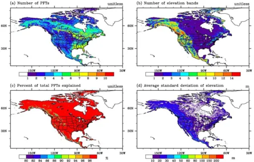
!_!"#$$₌₂₄

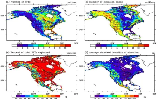
Fig. 4.Optimal classification SGC with maximum-allowed total classes N class₌24 at 0.1◦

resolution.(a)number of dominant PFTs classified for each grid;(b)number of elevation bands classified for each grid; (c) total percentage of PFTs explained by the method; (d) average standard deviation of elevation in each elevation bands in each model gridσ_ep.

(29)