SafeBox: adaptable spatio-temporal generalization for location privacy protection

SafeBox: adaptable spatio-temporal

gen-eralization for location privacy protection

Sergio Mascetti, Letizia Bertolaja, Claudio Bettini

E-mail:{sergio.mascetti, letizia.bertolaja, claudio.bettini}@unimi.it

Abstract. Spatial and temporal generalization emerged in the literature as a common approach to preserve location privacy. However, existing solutions have two main shortcomings. First, spatio-temporal generalization can be used with different objectives: for example, to guarantee anonymity or to decrease the sensitivity of the location information. Hence, the strategy used to compute the generalization can follow different semantics often depending on the privacy threat, while most of the existing solutions are specifically designed for a single semantics. Second, existing techniques prevent the so-calledinversionattack by adopting a top-down strategy that needs to acquire a large amount of information. This may not be feasible when this information is dynamic (e.g., position or properties of objects) and needs to be acquired from external services (e.g., Google Maps).

In this contribution we present a formal model of the problem that is compatible with most of the semantics proposed so far in the literature, and that supports new semantics as well. OurBottomUp

algorithm for spatio-temporal generalization is compatible with the use of online services, it sup-ports generalizations based on arbitrary semantics, and it is safe with respect to the inversion attack. By considering two datasets and two examples of semantics, we experimentally compareBottomUp

with a more classical top-down algorithm, showing thatBottomUpis efficient and guarantees better performance in terms of the average size (space and time) of the generalized regions.

1

Introduction

Emerging applications in the area of mobile and pervasive computing have significantly increased the risk of privacy threats by the uncontrolled release of information about the whereabouts of individuals. This information is not only released by the individuals them-selves while using their mobile phones or wearable sensing technology, but in some cases it is published by other users in social applications or transferred by providers to third par-ties. The collection of information about the presence of individuals in certain places at given times can lead to information about their movements, behavioral habits, and can po-tentially be used for unsolicited advertisement, discrimination and even stalking attacks. This risk is not only theoretical: for example, the work of Fattori et al. shows how it is possible (and relatively easy) to violate users’ privacy in existing real-world friend-finder services [7].

the reported geographical area. Temporal generalization introduces uncertainty about the precise time of presence of the user in the reported area, and is usually implemented by delaying the release of the spatio-temporal information and providing a temporal interval or using a coarser granularity instead of a precise timestamp. In this paper we callSafeBox

the spatio-temporal region used to generalize a source point representing the user’s exact location and time of presence.

The Problem

A crucial issue for this approach is deciding how large the SafeBox should be in order to avoid a privacy breach. This decision is not only important for privacy protection, but it also has an impact on the performance and precision of the service being used. The min-imum size of the SafeBox is actually dependent on the context, including the individual’s privacy preference, the application being considered, the time and place of service requests, the adversary model and other parameters. For example, solutions aimed at protecting identity privacy in LBS and adopting techniques inspired byk-anonymity(e.g., [8, 12, 11] ), have the goal to identifythe smallestSafeBoxes that contain at leastkother users in addition to the issuer of a LBS request that may potentially use the same service; by releasing the SafeBox instead of the exact position, a form of anonymity is enforced, since the released information by itself cannot be used to re-identify the individual, even in the case in which the adversary knows the identity of all the users in the reported area. Other generalization solutions, not focused on identity privacy but more on hiding the presence of an individ-ual in a potentially sensitive place (e.g., [6]) have a different optimization criteria for the dimension of their SafeBoxes. In some cases they wantthe smallestregions that include at leastkother venues, as pubs, shops, offices, in order to enforce uncertainty about the actual venue where the user is/was located. Increasing the temporal size helps keeping the spa-tial size small but it should satisfy the real-time constraints that the considered application may have.

Each of the proposed techniques is somehow specialized to optimize the generalization with respect to the specific semantics of privacy preservation (counting users, venues, cat-egories of venues, . . . ). Hence, one problem we would like to address in this paper is to have a generalization scheme solution that is parametric with respect to acounting function, and hence independent from the actual semantics of privacy preservation.

and separate calls are needed to get details (e.g., the opening hours). Each call can require up to2seconds to have a response, depending on the connection, and, moreover, only1000

calls can be performed daily without special permissions. In this scenario, evaluating pri-vacy conditions based on counting may become impractical with generalization strategies that operate top-down, because counting for large areas may be very time-consuming, if possible at all.

Hence, the second problem we are addressing in this paper is devising a new method to compute the SafeBox, compatible with the typical constraints involved in querying external services to obtain updated information on geo-referenced objects.

Contribution

Our solution to the second problem described above is a generalization algorithm that operatesbottom-up: It builds the SafeBox starting from the actual position and timestamp of the user, and, by adopting a specific data structure, recursively enlarges the spatio-temporal region until the counting constraints are satisfied, while maintaining protection against the “inversion” attack.

The main contributions of this paper are the following:

• By providing a general notion of object counting function supporting different se-mantics we capture in a single problem formalization several location privacy prob-lems previously considered in the literature and enable capturing privacy preferences not considered in previous generalization approaches.

• We design a generalization algorithm supporting arbitrary counting functions that operates bottom-up, enabling the verification of privacy conditions through public online services. To our knowledge this is the first safe generalization algorithm adopt-ing a bottom-up strategy.

• We implemented the BottomUpalgorithm and applied it to two different datasets, presenting a detailed comparison in terms of precision and performance, both with its top-down counterpart and with algorithms proposed in related work. The results confirm that our algorithm is effective, superior, and possibly the only alternative when access to updated external data is limited.

The rest of the paper is structured as follows. In Section 2 we discuss related work. In Sec-tion 3 we formalize the privacy problem and we define the two semantics of the counting function that we use in our experimental evaluation. Section 4 presents the newBottomUp

algorithm and compares it with one following the more traditional top-down approach. The experimental evaluation is reported in Section 5, and Section 6 concludes the paper.

2

Related Work

Some contributions in the literature adopted spatio-temporal generalization to enforce users’ anonymity while others used this technique to decrease the sensitivity of location informa-tion. One of the first techniques aimed at guaranteeing anonymity through spatial and temporal cloaking was proposed by Gruteser and Grunwald [10]. The idea is to guarantee a form ofk-anonymity in such a way that the issuer of a location-based service request cannot be identified.

“inversion” or “reciprocity”, has been addressed in [12, 11]. These two papers propose two analogous formal properties of the generalization function. Intuitively, a generaliza-tion funcgeneraliza-tionG meets these properties if each point contained in any generalized region

rcomputed byG is generalized toritself. The two papers prove that, if a generalization algorithm meets this property, then it is safe with respect to the inversion problem. In this contribution we propose a different property (see Section 3) that intuitively states that a generalized regionr computed by a generalization function G should contain at least k

objects that, if used as source points, are generalized toritself. The difference is that, in this new property, we only require that some points ofr(i.e., not necessarily all of them) generalize toritself. Hence this is clearly a looser property to meet but, as we prove in this contribution, it still guarantees the safety of the generalization algorithms with respect to the inversion problem. This new definition is required by ourBottomUpalgorithm that does not meet the properties defined in [12, 11] but instead meets the new property de-fined in this contribution and hence it is safe with respect to the inversion problem. The main problem with the generalization algorithms proposed in [12, 11] is that both require the knowledge of all the objects to be counted and hence are impractical when retrieving this information is costly, like, for example, in one of our experimental settings (see Sec-tion 5.3.4).

Other solutions proposed in the literature present the problem above. Among the others we can mention the technique proposed by Gedik et al. that has the advantage of allowing each user to choose a personalized value ofk[8], the solution by Abul et al. that makes it possible to anonymize a dataset of trajectories [1] and the solution by Mascetti et al. that addresses the issue of anonymity in location based services when different requests can be associated to the same user [13].

In the contribution by Ghinita et al. the objective of the spatial generalization is not to provide anonymity rather to decrease the sensitivity of the location information [9]. The technical problem is that, given two generalized spatio-temporal regions representing the location of a user, an adversary can be able to exclude part of them as possible user position if the maximum velocity for that user is known. The solution by Ghinita et al. does not investigate how the generalized spatio-temporal regions should be created, which instead is the focus of our contribution. We believe that extending our solution with a technique like the one presented in [9] is an interesting future work.

Other contributions share the same objective of decreasing the sensitivity of the location information. Some of them are specifically designed for the so-called friend-finder services [14, 16, 18] while others focus on how to let the user specify the desired level of privacy pro-tection [2]. None of these contribution focus on how to create generalized spatio-temporal regions that contains a minimum number of objects.

problem.

Finally, the solution by Damiani et al., takes into account the “semantic location” i.e., specific locations where the user does not want to be reported [6]. This is an innovative approach and it has two main differences with respect to ours. First, the generalization ap-plies to the entire map and is computed off-line. Vice versa, in our solution we generalize the location of the user on-the-fly, so the generalization function can use dynamic infor-mation. The second difference is that in the solution by Damiani et al. a user’s location is generalized only if it falls into an “obfuscated location” i.e., a sensitive location or its sur-roundings. This can lead to disclose which are the sensitive locations of a user, which we believe should be considered private information. To avoid this problem, in our solution we propose generalization functions that can be used to generalize requests from every location.

3

Problem Formalization

We address the problem ofgeneralizingthe information about a specific location and times-tamp into a geographical area and a time interval so that the resulting spatio-temporal information is still useful to obtain geo-referenced and timely services but not sensible any-more in terms of privacy. Since privacy is a subjective matter, the way generalization occurs not only has to be safe but should also be adapted to the user preferences. Our framework captures all preferences that can be expressed as a guarantee of presence in the released area of enough elements to sufficiently decrease the sensitivity of the spatio-temporal in-formation being released.

In the following of this section we first formally describe the general problem and then discuss the properties of the SafeBoxes that our techniques can return, depending on the different semantics associated to the function used to count the elements they contain.

3.1

Adversary model

The generalization techniques proposed in this contribution can be used to protect users’ privacy in different system architectures. Indeed, the generalization function can be com-puted either by the user’s mobile client or by a trusted generalization server. In both cases, the source point (i.e., the exact user’s position at a certain time) is not disclosed to any non trusted entity. Instead, the generalized location is disclosed.

The “adversary” is any entity that can potentially have access to the generalized spatio-temporal location. It can be, for example, a provider of a Location Based Service (LBS), an eavesdropper that intercepts the communication towards the LBS service provider, a hacker that violates the service provider system hence acquiring its stored data or even a govern entity that forces the service provider to disclose its stored information.

SafeBox), they can either be system parameters (hence easily discovered by an adversary) or, more likely, user-defined parameters. In the latter case it is still possible for an adver-sary to infer their value, possibly with some form of approximation (consider Example 1). Finally, for what concerns the knowledge of the counting function, in some case this can be public information (as in Example 1) and, if not, it can be inferred, possibly introducing some approximation in the computation, like in Example 1.

Example 1. Alice uses a privacy-aware LBS. Before issuing any service request, the client generalizes Alice’s spatio-temporal location so that it contains at leastkopen shops where

kis a user-defined parameter having values in[2,20].

Suppose that an adversary can observe a request issued by Alice from a generalized spatio-temporal regionA. Since inA there are6 open shops, the adversary can exclude that the parameterk chosen by Alice is larger than6. The adversary can also compute that, for any value ofk in[2,4], any request issued from a source point p ∈ Awould be generalized to region smaller thanA. Hence the value ofkis either5or6.

Now, suppose that the generalization algorithm used to generateAis not safe. It could happen that, for a given pointp∈ A, a request issued frompwith value ofkequals to5

returns an area different fromAand that the same holds for a request issued frompwith

k= 6. In this case the adversary can excludepfromI(A)even without knowing the exact value ofk.

It is important to note that in this paper we consider the spatio-temporal generalization of single requests and we do not address the problems arising when correlation among different requests is possible. Consequently, the direct application of our techniques is subject to two attacks known in the literature.

The first is the “velocity attack” that can lead the adversary to exclude the presence of the user in a given area at a given time, hence possibly restricting the generalized spatio-temporal region [9]. Since at the moment our generalization algorithms do not provide protection with respect to the velocity attacks, they should not be used in case of continu-ous disclosure of location information. Indeed velocity attack is ineffective if the location information is sporadically disclosed.

The second attack is aimed at violating “historical k-anonymity” and takes place when the counting function is used to count the users and is aimed at guaranteeing the issuer’s anonymity [13]. In this case, if it is possible to “link” different generalized regions to the same (anonymous) user, the adversary can intersect the “anonymity sets” hence possibly restricting the possible identity of the user to a set with cardinality smaller thank. Since our generalization algorithms do not take this attack into consideration, if the counting function is used to count users with the aim of providing anonymity, it should be guaranteed that no set of generalized regions can be associated to the same user for example by artificially changing the IP address used in the corresponding service requests.

3.2

Basic definitions

We assume that users and (possibly moving) objects are located in a finite bi-dimensional spatial domainSand we consider their positions in a finite interval of timeT. We denote withS1 andS2 the two dimensions ofS and withpa spatio-temporal point (or “point”, when no confusion arises). Formally,p∈S×T =S1×S2×T.

One of the required properties for the generalization is to guarantee that the resulting area “contains” at leastkobjects. We use the function Ωto count the number of objects contained in a given area. Formally, given a set of (possibly moving) objects and a spatio-temporal areaA,Ω(A)is a non-negative integer value representing the number of spatio-temporal points corresponding to positions and associated timestamps of the objects inA. The counting functionΩ(A)can also be applied whenAis a set of possibly non-contiguous spatio-temporal points. The specification ofΩincludes the set of objects to be considered (e.g., users, shops, taxis, etc.) as well as the actual semantics of the counting operator. In Section 3.3 we report two examples of its semantics. Note that the source point being generalized can be the position of one of the objects (as in the case of the source point is the position of a user and the objects are all users) but can also be an unrelated point (as in the case of objects being pubs and the user not being positioned in any of them). Note also that the results we present in this paper assume only that the counting function is monotonic with respect to the areas.

Definition 2. A counting functionΩis monotonic if, for each pair of spatio-temporal areas

AandA′_{such thatA⊆A}′_{it holds thatΩ(A)≤Ω(A}′_).

Monotonicity captures an intuitive property. For example, if in the main square of a city there are100 people at given moment, by considering at the same moment a larger area that includes the square, we will count100or more people.

When a spatio-temporal area contains at leastk objects, we say it is a “SafeBox”. Intu-itively, the user considers herself to be “safe” by releasing this spatio-temporal information because the source pointpcan be confused with the positions and timestamps associated to at leastkobjects.

Definition 3. Given a non-negative integerkand a counting functionΩ, a spatio-temporal areaAis aSafeBoxifΩ(A)≥k.

As observed in the literature [11, 12], even if a generalization function returns a SafeBox according to Definition 3, an adversary may still be able to rule out some of the objects considered in the counting if he knows the generalization function itself, since he may re-apply the generalization function to each candidate source point and compare the result with the area that has been released. In principle, by knowing the generalization function the adversary may also be able to identify the source pointpthough the so calledinversion attack[12]. Consider Example 4.

Example 4. Let’s consider Figure 1: the spatial and temporal domain is partitioned into four areas. The number in the top right of each area represents the value of Ω(). The objective of the generalization is to have a SafeBox with at least8objects. Let’s consider a naive generalization function that, given any source point inA2, generalizes it toA2. Similar forA3. SinceΩ(A1)is less than 8, A1 is not a SafeBox and hence the algorithm generalizes any source point inA1 to the SafeBoxA1∪A2. Similarly, any source point in

A4is generalized toA3∪A4.

Now, consider an adversary that knows the generalization function and the values ofΩfor each area. If this adversary observes the SafeBoxA1∪A2than he can exclude that the source point is inA2, because in this case the generalization would beA2itself. Consequently the adversary infers that the source point is inA1that, however, is not a SafeBox.

A

A

A

A

20 5

Figure 1: Spatio temporal domain partitioned into four areas.

Definition 5. Given an areaAand a generalization functionG, theinversionfunctionIis defined as:

IG(A) ={p∈A|G(p) =A}

When no confusion arises, we simply denoteI(A)omitting the generalization function. We can now define the notion of safety for generalization functions.

Definition 6. Given a non-negative integerkand a counting functionΩ, a generalization functionGissafeif, for each spatio-temporal pointpsuch thatG(p)is defined, it holds that:

Ω(I(G(p)))≥k

Example 7. Let’s continue with Example 4. We show that the generalization function is not safe according to our model. Indeed, for any pointpinA1, the generalization of that point isA1∪A2. The inversion ofA1∪A2isA1(indeed the generalization of any point inA2is

A2itself). Consequently,Ω(I(G(p))) = Ω(A1) = 5<8. Consequently, by applying Defini-tion 6, the generalizaDefini-tion funcDefini-tion is not safe, in accordance with the intuiDefini-tion presented in Example 4.

Let’s now consider a different generalization function that generalizes any source point ofA2inA2and similar forA3. Also, the generalization of any source point inA1orA4is the entire spatio-temporal domain (i.e.,A). This is actually a safe generalization function. Indeed, for any source pointpin A2 it holds that its generalization isA2 and also that

I(A2) = A2. ConsequentlyΩ(I(A2)) ≥ 8. Similar forA3. Vice versa, for any pointpin

A1andA4, the generalization yieldsA. In this caseI(A) =A1∪A4. Hence we have that

Ω(I(G(p))) = Ω(A1∪A4) = 10≥8. Note that in this last case (i.e., any source point inA1or

A4), it is actually possible to use the inversion attack to restrict the area (fromAtoA1∪A4), but this does not affect the safety of the technique, sinceA1∪A4still contains a sufficiently large number of objects.

Property 1. Any safe generalization functionG returns a SafeBox for any source pointp

such thatG(p)is defined.

Proofs of formal results are reported in Appendix A.

3.3

Supporting different semantics for the counting function

Ω

the sensitivity of the location information. Also, by counting different types of shops, it is possible to enforce a property similar tol-diversity.

In the following we first specify theappearancesemantics (that can be used for example to guaranteek-anonymity) and then we specify thepersistencethat is original, to the best of our knowledge.

3.3.1 Appearance semantics

This semantic captures the counting of distinct objects that happen to be within a spatial areaAS in any time instant during a temporal interval AT. Each object is “counted” if

it happens to be located withinAS at least during one time instant ofAT. Each object is

counted at most once, independently from how much time it spends withinAS and even

if the object enters and exits several times fromASduringAT.

In order to define this semantic, we first introduce the functionloc()that we use to model the position of an object at a given time instant.

Definition 8. Given the setOof objects we define a partial functionloc:O×T →Ssuch that,loc(o, t)is the spatial position of objectoat timet.

We are now ready to define theappearance counting semantics.

Definition 9. Given the set of objectsO, an areaAand its projectionsAS,AT on the

spa-tial and temporal domain, respectively, thecounting functionΩwithappearance semanticsis defined as follows:

Ω(A) =|{o∈Os.t.∃t∈AT withloc(o, t)∈AS}|

Example 10. Suppose thatASis a city’s park andAT is from 2 pm until 2.30 pm. Given that Ois the set of users of a location based service, theΩ()counting function with appearance semantics counts how many of these users report their location in the park at least once between 2 pm until 2.30 pm.

Any specification of theΩ()counting function should be shown to be monotonic for our algorithms to be sound.

Property 2. The counting functionΩ()with appearance semantics is monotonic.

3.3.2 Persistence semantics

According to the appearance semantics each object is counted once independently on how long it has been located within the spatial areaAS during the time intervalAT. In some

applications it can be desirable to count more than once those objects that are located in

AS for a “sufficiently long time” duringAT. This semantics captures the intuition that

a spatio-temporal area containing some shops for a period of2hours provides more pri-vacy protection than a spatio-temporal region that contains the same shops but that has a duration of10minutes.

Given a persistence interval duration D, the intuition of the persistence semantics is to count, for each object, for how many persistence intervals duringAT that object is located

inAS.

Definition 11. Given the set of objectsO, an areaAwith its projectionsAS,AT on the

spa-tial and temporal domain, respectively, andIthe set of persistence intervals with duration

D, thecounting functionΩwithpersistence semanticsis defined as follows:

Ω(A) =X

o∈O

|{i∈Is. t.∃t∈(i∩AT)andloc(o, t)∈AS}|

Example 12. Suppose we are computingΩ()for the center of Milan, for the interval from

7pmto11pmof a given day, counting the number of open pubs. A pub that is always open in this time interval is counted4times if the persistence interval durationDis1hour. IfD

is15min it will be counted16times, but it will be counted14times ifDis15minutes and it closes at10:30. Intuitively, the pub may be a possible location for the user in each of the persistence intervals contained in the considered temporal interval if it is actually open at that time. The condition on the opening time is captured in Definition 11 by the predicate

loc(o, t)∈AS. The number of persistence intervals intuitively gives a value for a “temporal

obfuscation” metrics.

Property 3. The counting functionΩ()with persistence semantic is monotonic.

4

SafeBox computation

In this section we present two safe generalization algorithms that share the main data struc-ture, that we callgeneralization tree, but have a different conceptual approach to the gener-alization process.

TheTopDownalgorithm starts by considering the entire space and time (the “top”) and then “moves down” from the root of the generalization tree searching for a node corre-sponding to the “smallest” spatio-temporal region that guarantees the safety property of the algorithm. In contrast, theBottomUpalgorithm starts from the leafs of the generaliza-tion tree, which intuitively correspond to small spatio-temporal regions, and then “moves up” in the tree with the same goal.

TheTopDownalgorithm is conceptually more intuitive and, as we will see later, it also has a lower worst-case complexity. The spatio-temporal generalization algorithms proposed so far for location privacy follow this approach. As we detail in this section, guaranteeing the safety property by following theBottomUpapproach is more challenging. However, considering that the counting function must be computed for any candidate region, the

BottomUpalgorithm has the advantage of being a “local” algorithm, in the sense that in many cases it terminates after processing data located in a small spatio-temporal area. Vice versa,TopDownalways starts from the entire spatio-temporal domain and hence it requires information on all the objects.

In the following of this section we first formalize the generalization tree in Section 4.1, and then we present theTopDownandBottomUpalgorithms in Sections 4.2 and 4.3, respectively.

4.1

Data structure: the generalization tree

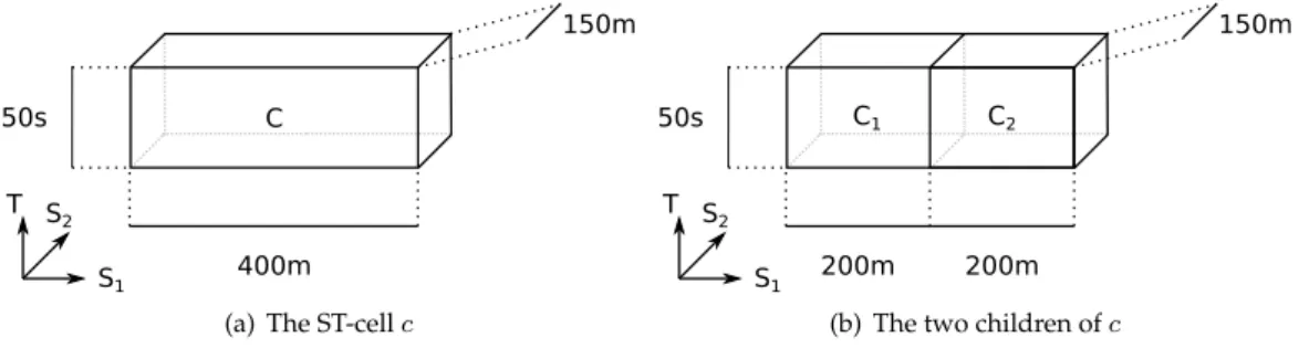
system parameter and the ST-cell associated with the root is the entire spatial and temporal domain (i.e.,S×T). The ST-cell of each non-leaf node is partitioned by the ST-cells of its two children as detailed in the following. Given this construction, it is easily seen that the nodes at a given level partitionS×T.

We now specify how to construct the two children{c1, c2} of any internal nodecin the generalization tree. Intuitively, we splitcalong one of the three dimensions, dividing it in two even parts. Since the two resulting cellsc1 andc2 partitionc, their projection on the other two dimensions is the same as inc, as shown in Figure 2.

S1 S2 T

400m

150m

50s C

(a) The ST-cellc

S1 S2 T

200m

150m

50s C1 C2

200m

(b) The two children ofc

Figure 2: A ST-cellcand its two childrenc1andc2

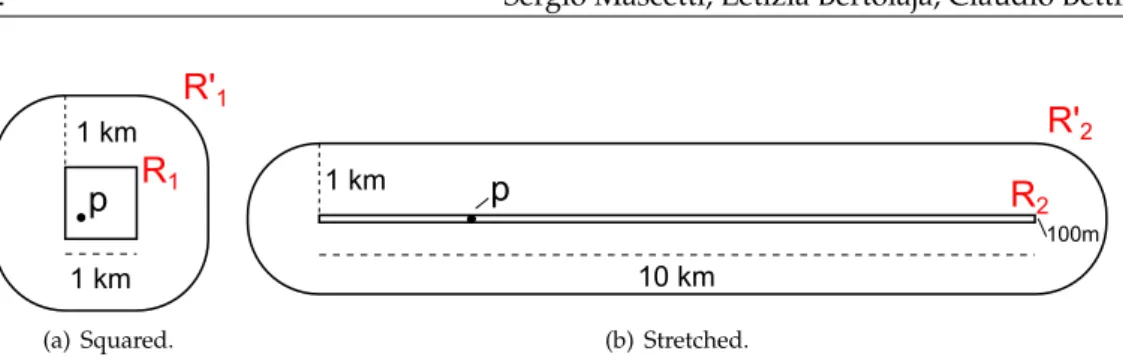
In order to decide along which dimension a cell should be divided, we follow the intu-itive goal of preferring squared ST-cells over stretched ones. We explain this intuition with Example 13.

Example 13. Alice is using a fiend-finder service to be notified when one of her friends is closer than1km. The service is “privacy-aware” and it is designed to receive generalized locations from the users.

To protect Alice’s privacy, her client always generalizes Alice’s location to a regionR con-taining10shops. The server replies with the set of friends closer than1km to any point of

R. Finally the client filters out those friends whose position is not actually closer than1km from the exact Alice’s location.

Suppose that, for a give source position p, there are two different generalization algo-rithms: one returns a squared regionR1, the other the stretched regionR2(see Figures 3(a) and 3(b)). Note that the two regions have the same area of1km2

. Upon receivingR1 and

R2, the service provider would return the friends in the regionsR′

1andR′2, respectively,

withR′

2being more than3times larger thanR′1. Consequently we can expect, on average,

that the generalization toR2incurs into larger communication costs and larger computa-tional costs both on the client and on the server.

p

1 km 1 km

R

R'

(a) Squared.

p

10 km

100m

1 km

_R

2

R'

(b) Stretched.

Figure 3: Comparison between a squared generalized region and a stretched one.

In the following definition, we use the notation|c|Dto denote the projection of a ST-cellc

along dimensionD.

Definition 14. The split dimension of an ST-cell c with time influence parameter α ∈

[0; +∞), denoted withsplitα(c)is defined as:

splitα(c) = 

 

 

S1 if|c|S1≥ |c|S2 and|c|S1≥α· |c|T S2 if|c|S2>|c|S1 and|c|S2≥α· |c|T T otherwise

Finally, we formalize how children are constructed.

Definition 15. Letc be an ST-cell,D1 =splitα(c)be the split dimension ofc,D2 andD3

the other two dimensions,|c|D1 = [min, max)and med =

max+min

2 . Then, the function

childrenα(c)returns the two childrenc1andc2ofcdefined as follows:

|c1|D1 = [min, med)

|c2|D1 = [med, max)

|c1|D2 =|c2|D2 =|c|D2

|c1|D3 =|c2|D3 =|c|D3

In the following, to shorten the notations, given a ST-cell c we denote withsibα(c)its

sibling, and withparα(c)its parent. In these notations we omitαwhen no confusion arises.

4.2

The

TopDown

algorithm

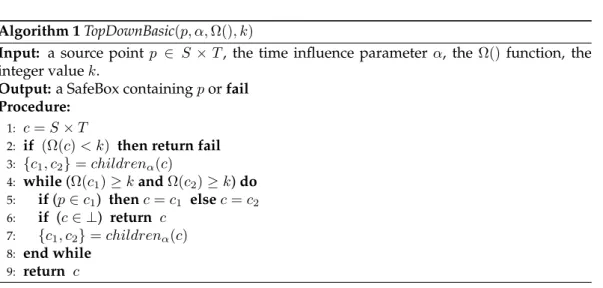
The intuitive idea behind theTopDownalgorithm is to traverse the generalization tree from the root towards the leaf node that contains the source point. The algorithm terminates when it reaches that leaf node or an internal nodecsuch that the counting function of one the children ofcyields a value smaller thank. As shown in the proof of Theorem 20, this termination condition makes this generalization function safe. The basic version of the algorithm is shown in Algorithm 1.

Example 16. Consider a generalization tree like the one in Figure 4. The number reported in each leaf ST-cell indicates the value ofΩfor that ST-cell. Also, consider a source pointp

Algorithm 1TopDownBasic(p, α,Ω(), k)

Input: a source pointp ∈ S×T, the time influence parameter α, the Ω() function, the integer valuek.

Output:a SafeBox containingporfail Procedure:

1: c=S×T

2: if (Ω(c)< k) then return fail

3: {c1, c2}=childrenα(c)

4: while(Ω(c1)≥kandΩ(c2)≥k)do

5: if(p∈c1) thenc=c1 elsec=c2

6: if (c∈ ⊥) return c

7: {c1, c2}=childrenα(c)

8: end while

9: return c

TopDownBasicfirst considers the rootC. Since the value ofΩ(c)for the whole domain is equal to12(the sum of the counting function among all leaf ST-cells), the algorithm does not terminates here with failure (see Line 2) but instead computes the two children ofC

(Line 3). The condition for entering in the loop (see Line 4) is then considered: since ST-cell

C2is such thatΩ(C2)<4, then the algorithm does not enter the loop andCis returned in Line 9 as the SafeBox.

0 1

C7 C8 C9 C10 C11 C12 C13 C14

C3 C4 C5 C6

C1 C2

C

3 4 2 1 1 1

Figure 4: Example of generalization tree

Note thatTopDownBasicreturnsfailonly whenkis larger than the total number of objects to count in the entire spatio-temporal domain. Indeed, in this case it is impossible to find a SafeBox, independently from the generalization function. Vice versa, in all other cases (i.e., whenΩ(S×T)≥k),TopDownBasiccan always find a SafeBox.

Algorithm 1 has a computational issue: each time the algorithm moves one level down in the generalization tree from a ST-cellc, it needs to recompute Ωover the two children of

Algorithm 2 shows the pseudocode for TopDown. Variable c represent the current ST-cell being processed that is set to the entire spatio-temporal domain in Line 1. Then the algorithms enters in awhile loop that traverses the generalization tree towards the leaf ST-cell containing the source pointp. At each iteration, unless the algorithm terminates at that iteration, it only evaluatesΩfor the childc2ofc that does not containp(Line 9). Indeed, ifΩ(c2) ≥ k, the algorithm does notdirectlycheck ifΩ(c1) ≥ k, where c1 is the child ofc containingp. Instead, the algorithm processesc1in the following iteration. If theΩfunction applied to a child ofc1yields a value not smaller thank, then, due to the monotonic property ofΩ(see Definition 2)Ω(c1) ≥ k. In practice, with this approach in most of the cases (i.e., all the cases in which the algorithm continues in the iteration) we have anindirectevaluation of the conditionΩ(c1)≥k.

WhenΩ(c2)< kwe cannot indirectly infer ifΩ(c)≥kand the algorithm explicitly needs

to compute this condition (see Lines 11 to 15). IfΩ(c)≥kthen the result iscitself. Other-wise, due to the termination condition ofTopDownBasic, the result is the parent ofc. In casec

is the entire spatio-temporal domain (i.e., the root of the generalization tree), the algorithm returnsfail. This happens only when theΩfunction applied to the entire spatio-temporal domain yields a values smaller thank.

Finally, there is another termination condition: when the algorithm reaches a leaf ST-cellc

(see Lines 3 to 6). Also in this case it is not possible to indirectly evaluate ifΩ(c)≥k, hence the algorithm explicitly compute this condition and it returnscif the condition is met, the parent ofcotherwise.

Algorithm 2TopDown

Input: a source pointp ∈ S×T, the time influence parameter α, the Ω() function, the integer valuek.

Output:a SafeBox containingporfail ProcedureTopDown(p, α,Ω, k)

1: c=S×T; 2: while true do

3: if(c∈ ⊥)then

4: if(Ω(c)≥k)then returnc

5: else then returnparentα(c)

6: end if

7: c1is the ST-cell inchildrenα(c)such thatp∈c1

8: c2is the ST-cell inchildrenα(c)such thatp6∈c2

9: if(Ω(c2)≥k)then

10: c=c1 11: else

12: if(Ω(c)≥k)then returnc

13: else if(c=S×T)then return fail

14: else returnparentα(c)

15: end if

4.3

The

BottomUp

algorithm

TheBottomUpalgorithm processes the generalization tree from the leaf node containing the source point towards the root.

An intuitive procedure would first identify the leaf node containing the source pointpand recursively move to the parent ST-cell in case the value ofΩfor that ST-cell is less thank, and returning the current node as the SafeBox whenΩis at leastk. We proposed a similar algorithm, calledIncognitus, in a preliminary investigation on this problem [4]. Unfortu-nately, the result obtained with this approach is indeed aSafeBox, but the generalization function is not safe according to our definition, as shown in Example 17.

Example 17. Consider the generalization tree reported in Figure 5, a value ofkequal to4

and a bottom up generalization algorithm that, starting from the leaf ST-cell containing the source point, continues to generalize if the value ofΩfor the current ST-cell is less thank.

C11 C12 C21 C22

C1 C2

C

1 1 5 1

p1

p2

Figure 5: Unsafety of an intuitive bottom-up strategy

The generalization of p1 isC21, since Ω(C21) = 5 ≥ k. If the source point is p2, the algorithm first processesC11but discards this as a SafeBox, becauseΩ(C11) = 1< k. Then the algorithm moves up in the tree, processing ST-cellC1. This is not a suitable SafeBox neither, sinceΩ(C1) = 2 < k. Then the algorithm moves up to cthat is a SafeBox since

Ω(C) = 8≥k.

This algorithm has the same problem illustrated in Example 4. Intuitively, by observing a generalization toC, an adversary may exclude as a candidate source point any point in

C21(since it would be generalized only toC21). Hence the privacy preference of having at leastkobjects around the source point would be violated. Technically this is captured by the fact thatI(C0) =C11∪C12∪C22. SinceΩ(C11∪C12∪C22)< k, this algorithm is not safe.

We first formally describe theBottomUpalgorithm, and then we provide an example of its application. Algorithm 3 starts from the leaf ST-cell containing the source pointp(Line 1) that is also assigned to variablecused in the main loop. IfΩfor that ST-cell is greater than or equal tok, the algorithm returns that ST-cell, since for leaf nodesI(c) = cifΩ(c) ≥ k

(Line 8). If this is not the case, the algorithm enters in thewhile loop that traverses the generalization tree towards the root. If the algorithm actually reaches the root without finding a node that satisfies the termination condition, then it fails since it is not possible to obtain a SafeBox for the given source point with the considered procedure (Line 4). Note that this implies that in some casesBottomUpcould not be able to find a SafeBox while a different algorithm (e.g.,TopDown) actually could. However, this a very rare situation (see Section 5).

Vice versa, if the considered ST-cell (currentST cell) is an internal node, its value is up-dated with the one of its parent node in the generalization tree (Line 5), and the count-ing function is evaluated on the inversion of this new ST-cell, computed through the Bot-tomUpInversionfunction (presented in the following).

Algorithm 3BottomUp

Input:a source pointp, a time influence parameterα, theΩ()function, the integer valuek.

Output:a SafeBox containingporfail Procedure:

1: currentST cellis the leaf ST-cell such thatp∈currentST cell

2: c=currentST cell

3: while(Ω(c)< k)do

4: if(currentST cell=S×T)then return fail

5: currentST cell=parα(currentST cell)

6: c=BottomUpInversion(currentST cell, α,Ω, k)

7: end while

8: return currentST cell

Example 18. Let’s consider again the generalization tree in Figure 4. As in Example 16 the goal is to find the SafeBox containing at least4objects. TheBottomUpalgorithm starts computing the leaf ST-cell containingpin Line 1 (identifying the ST-cellC7shaded in grey in Figure 4). Then it computes the valueΩ(C7) = 3; since the requirement of having at least

4objects is not fulfilled, the algorithm enters the while loop (Line 3). SinceC7 6=S ×T, the algorithm computes the parent ofC7 in Line 5, considering as candidate SafeBox the ST-cellC3in Figure 4. The inversion ofC3, computed by theBottomUpInversionprocedure (Line 6), is the empty set: indeed,C3is the union ofC7andC8, and any point inC8would have as SafeBoxC8 itself because itsΩ()is equal to4. Furthermore any point inC7will have as SafeBox an area greater than the one represented byC3, because otherwise the only candidate source points for the generalization toC3will be the one inC7and the counting in that area is insufficient to guarantee the user privacy preferences. Since the counting for an empty set is zero, the algorithm enters again in the loop. SinceC3 6=S×T the parent ofC3is computed asC1. The inversion ofC1is the union ofC7,C9, andC10since both the

Ωvalue ofC9andC10and theΩof their unionC4are smaller than4, and hence, any point in those ST-cells would have as SafeBox the region corresponding to the nodeC1or to an ancestor ofC1. It is indeedC1 because the counting function gives a value higher than4

algorithm to exit the loop, returningC1as the SafeBox.

Note that in Example 18 we just gave an intuitive motivation for the result of the inversion computation. Two problems arise when trying to directly apply Definition 5 to compute

I(c)for a ST-cell c when the generalization function isBottomUp. First, according to the definition, it would be necessary to computeBottomUpfor each point inc, which is impos-sible if we consider a continuous spatio-temporal domain and impractical even assuming a discrete domain. Second, this would generate a non-terminating procedure. Indeed, ac-cording to Definition 5, for anyp∈cwe need to computeBottomUpwithpas a source point. However, the computation ofBottomUprequires computing the inversion for an area that containsp, which is clearly an endless recursion.

The first problem can be easily fixed. Indeed, in BottomUp all points belonging to the same leaf node are generalized to the same SafeBox. So, instead of checking the inversion property for each point in the current candidate SafeBox, we can choose a representative point for each leaf ST-cell in the candidate SafeBox and check the condition for these points only.

To solve the second problem (non termination), we adopt Procedure 4. The idea is that, instead of directly computing Definition 5, which applies to any generalization function, we adopt Procedure 4 that is specific forBottomUpand that, in the computation, does not require to recursively callBottomUpitself.

Procedure 4BottomUpInversion

Input:a ST-cellc, a time influence parameterα, theΩ()function, the integer valuek.

Output:IBottomUp(c)

ProcedureBottomUpInversion(c, α,Ω, k)

1: res=Residuals(c, α,Ω, k); 2: if(Ω(res)≥k) then return res

3: else return ∅

ProcedureResiduals(c, α,Ω, k)

1: if(cis leaf)then returnc

2: result=∅

3: for eachc′_inchildren α(c)do

4: A=Residuals(c′_{, α,Ω, k)}

5: if(Ω(A)< k) then result=result∪A

6: end for

7: return result

Our solution to compute I(c) consists in the BottomUpInversion procedure (see Proce-dure 4) that usesResiduals, a recursive procedure that computes the set of all points whose generalization is not smaller thanc. If the counting function applied to this set is larger than or equal tok, then this set is returned (Line 2). Indeed, all of these points (res) gener-alize toc. Otherwise, (i.e.,Ω(res)< k), the counting condition inBottomUpfor the points inresis not satisfied and hence the generalization of each of these points is larger thanc. In this case,∅is returned as required by the definition ofI(c).

c′_{ofc,Residualschecks if the counting function applied toResiduals(c}′_{, α,Ω, k)is less than} k. If this is the case, then every point in the result ofResiduals(c′_{, α,Ω, k)is added to the}

result that is being computed forc(Line 5). Otherwise, (i.e.,Ω(Residuals(c′_{, α,Ω, k))≥ k)}

every point inc′_{generalizes to a ST-cell smaller thanc, hence no point ofc}′_{contributes to}

the result.

Example 19. Let’s consider Example 18 that illustrates the application of the BottomUp

algorithm to the generalization tree in Figure 4, and in particular to a source pointpin the ST-cellC7. The algorithm requires the computation ofBottomUpInversion(C3)and of

BottomUpInversion(C1)that we intuitively motivated as equal to∅and to C7∪C9∪C10, respectively. Consider firstBottomUpInversion(C3) 1_{. TheBottomUpInversion procedure,}

first computes the setresthrough theResidualsprocedure. SinceC3is not a leaf, the inner iteration ofResidualsconsiders firstc′ _{=C7and thenc}′ _{=C8. Forc}′ _{=C7,A ={C7}, and}

sinceΩ(A)is less than4,C7is added toresult. Forc′ _{=C8,A={C8}, and sinceΩ(A)is}

greater than4,resultis not modified. TheResidualsprocedure returns the set containing onlyC7, so we have thatres ={C7}. SinceΩ(res)<4, theBottomUpInversionprocedure terminates returning the empty set.

Consider now the computation ofBottomUpInversion(C1). SinceC1is not a leaf, the inner iteration ofResidualsconsiders firstc′ _{=C3 and thenc}′ _{= C4. WhenResidualsconsiders} C3, as we have seen before, it returnsresult={C7}. Then it considersC4 and computes

A = C9 ∪C10 because both of these cells are leaves and the counting function applied to each of them is less than4. SinceΩ(A) = 3is less than4, the procedure returnsC9∪

C10. Consequently, Residuals applied to C1 returns result = C7 ∪C9 ∪C10. Hence in

BottomUpInversion(C1)we haveres =C7∪C9∪C10and sinceΩ(res) = 6, the procedure returnsC7∪C9∪C10, as expected from our intuitive reasoning in Example 18.

4.4

Properties of the

TopDown

and

BottomUp

algorithms

In this subsection we consider the formal properties of the two algorithms that we have presented and we compare their worst-case time complexity.

4.4.1 Safety

In order to show the correctness of the algorithms we have to prove that bothTopDown

andBottomUp compute a safe generalization function. ForTopDown, we first show that

TopDownBasicis a safe generalization function and then we show thatTopDowncomputes the same result asTopDownBasic(henceTopDownis a safe generalization function). This is formally stated in Theorems 20, 21.

Theorem 20. TheTopDownBasicalgorithm computes a safe generalization function.

Theorem 21. For any source pointp, any time influence parameterα, anyΩ()function, and any the integer valuekit holds thatTopDownBasic(p, α,Ω, k)=TopDown(p, α,Ω, k).

Before presenting the formal result forBottomUpin Theorem 22, we first present Property 4 that formally states thatBottomUpInversionactually computes the inversion forBottomUp.

Property 4. LetGbe the generalization function computed byBottomUpwith time influence parameterα, counting functionΩ(), and integer valuek. For each ST-cellc, BottomUpInver-sion(c,α,Ω(),k) computesIG(c).

Theorem 22. TheBottomUpalgorithm computes a safe generalization function.

The formal proofs of the above theorems are reported in Appendix A. Intuitively, the idea of both proofs is the following: we first show that if the algorithm does not returnfail, it returns a ST-cellc that contains the source pointp(this guarantees that the algorithm actually computes a generalization function) and then, according to Definition 6, we prove thatΩ(I(c))is not smaller thank.

4.4.2 Analysis of computational complexity

We first consider the worst-case time complexity. For each iteration of the main loop, the only operation inTopDownthat does not require a constant time is the computation ofΩ(). In the worst-case (i.e., when the algorithm returns a leaf node)TopDowncomputesΩ()once for each level of the tree. Hence the worst-case time complexity ofTopDownis linear in the height of the generalization tree times the complexity of computingΩ.

Before analyzing the complexity of BottomUp, we first introduce a simple but effective optimization. In principle the computation ofBottomUpInversion(c), as described in Proce-dure 4, would require to computeΩfor each node in the subtree with rootc. However, by definition ofBottomUp, ifcis an internal node, we computeBottomUpInversion(c)only if we have already computedBottomUpInversion(c′_{)for one childc}′_{ofc. By storing the result of} BottomUpInversion(c′_{), we avoid to re-process the subtree with root inc}′_{when computing} BottomUpInversion(c). With this optimization, we never computeΩ(c)twice for the same ST-cellc. Consequently, in the worst-case (i.e., whenBottomUptraverses the generalization tree up to the root), we need to computeΩfor each node in the tree.

Comparing the two algorithms, given a generalization tree of heighth,TopDownrequires computingΩa number of times linear inh, sinceTopDown“moves down” in the general-ization tree at each iteration. Vice versa, in the worst caseBottomUpneeds to process all nodes of the generalization tree, hence it is linear in the number of nodes (i.e.,2h_{) and,}

consequently, exponential inh. We recall that, by definition of the generalization tree (see Section 4.1), the height of the tree (and hence the number of its node) is a system parameter. The choice of a value forhis subject to a trade-off. On one side, for higher generalization trees we get smaller bottom ST-cell and this positively impacts on the average size of the generalization regions (this strongly affectsBottomUpand, minimally TopDown). On the other side, for larger values ofhwe have a higher computation time (again, this affects

BottomUpsignificantly and andTopDownonly minimally). In Section 5 we show the impact of this parameter in our experimental setting.

Let’s now consider the worst-case time complexity of the two algorithms by also taking into account the complexity of computing Ω. Clearly, the complexity of Ω depends on the data structure used to store the objects. In our experiments we use two different data structures. As we illustrate in Section 5, by using one of them we have a worst-case time complexity ofΩlinear in the number of leaf ST-cells contained in the considered area. With this data structure, we can evaluate the complexity of the two algorithms in terms of total number of leaf ST-cells that each algorithm needs to process in all the computations of

Ω. According to this metric, givenhthe height of the generalization tree, the worst-case time complexity ofTopDownisO(2h+1

). Indeed, in the first iterationTopDowncomputes

Ωon the entire spatio-temporal domain (i.e., 2h

leaf ST-cells), in the second iteration it computes omega on half of the spatio-temporal domain (i.e.,2h−1_{leaf ST-cells) and so on.}

Consequently, in the worst-case, the number of processed ST-cells isPh i=02

h

= 2h+1_−1.

The worst-case time complexity ofBottomUpisO(h·2h

computes omega for each node of the generalization tree. Since, the union of all the nodes at the same height yields the entire spatio-temporal domain (i.e.,2h

leaf ST-cells), the total number of ST-cells to process is equal toh·2h

. As a result, comparing the worst-case time complexity of the two algorithms,BottomUpis expected to be onlyh/2times slower than

TopDown.

5

Experimental evaluation

In this section we evaluate the SafeBox computation algorithms described in Section 4. Using two different datasets, we first evaluate the effectiveness ofTopDownandBottomUp

algorithms by showing how parameterkimpacts on the data quality, i.e., the spatial size and temporal duration of SafeBoxes. Intuitively, as long as a spatio-temporal region is a SafeBox, it should be as small as possible so as the approximation involved in its use is reduced. Secondly, we empirically evaluate the performance of the two algorithms in terms of computation time. Finally we compareTopDownandBottomUpwith our previous solutionGrid[12].

5.1

Experimental setting

The spatial area in which the experiments have been conducted is the city of Milano and the total size of the map is325 km2_{. In our experiments we use two datasets: the first}

represents the movement of a set of users, as described in Section 5.1.1, while the second dataset includes all the shops in Milano with opening hours (see Section 5.1.2). Hence the “objects” counted byΩ() will be users and shops, respectively. The choice of using different datasets is aimed at testing our algorithms with both dynamic and relatively static data. The results are computed as the average, as well as minimum and maximum, out of

1000runs. In each run, a random source point is chosen. The parameterkrepresents the minimum number of objects that each SafeBox returned by the algorithms should contain. Theαvalue, as described in Section 4.2, determines different ratios between the spatial and temporal sizes of the SafeBox. The choice ofαis strictly related to the application we are using: if we are in a real time environment we need to keep the temporal size, and hence temporal obfuscation, as small as possible, while in other contexts it could be useful to have smaller spatial areas or balance the space and time components. In all the experiments presented in this section we use a value ofα= 1.6×10−5_{such thatα·60s= 0.787km: this}

value, chosen empirically, produces SafeBoxes with a duration that is, on average, under

15minutes. This is a reasonable length if, for instance, we think about a service that uses the position for sharing purposes.

The two algorithms have been implemented in Java. Geographical positions are repre-sented as latitude and longitude values in decimal degrees. The experiments have been conducted is on computer with2.5GHz Intel i5CPU with4GB of main memory.

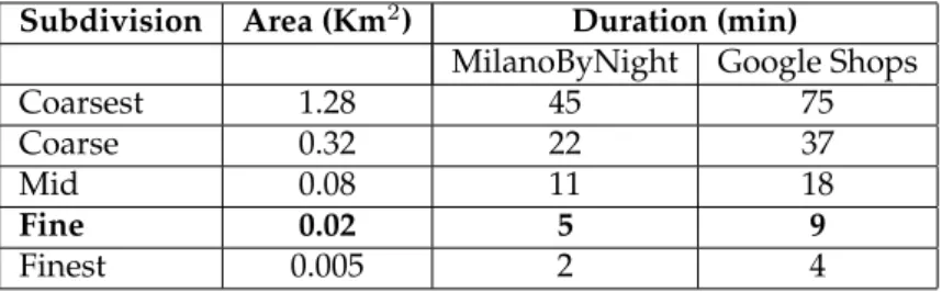
Subdivision Area (Km2

) Duration (min)

MilanoByNight Google Shops

Coarsest 1.28 45 75

Coarse 0.32 22 37

Mid 0.08 11 18

Fine 0.02 5 9

Finest 0.005 2 4

Table 1: Spatial and temporal leaf ST-cell size

5.1.1 MilanoByNight

MilanoByNight is an artificial dataset of user movements obtained using a simulation that reflects a typical scenario of a weekend night in the city of Milano. It includes100,000

potential users, moving to one or more entertainment places in a period of6hours2_.

The average density of the users within this area is465users/km2

. In this scenario, given a ST-cellc,Ωcounts the number of users withinc, according to the appearance semantics described in Section 3.3. In Table 2 the values ofkare summarized.

Parameter Values

k 20,40,60,80,100,120,140,160

Table 2: MilanoByNightkvalues

5.1.2 Google Shops

This dataset considers the same spatial area of MilanoByNight, but instead of considering users as the set of objects, it considers shops. The dataset includes12,958shops whose position and properties were retrieved through Google Places API. An opening timetable is assigned to each shop, using real values when available (about2,000shops) and assigning default opening times in the other cases. The considered temporal domain is10hours long, from9.00AM until19.00PM of a given day.

TheΩ()function counts theopenshops in candidate SafeBoxes. We test our algorithms with both the semantics described in Section 3.3: appearance and persistence. Important parameters for the experiments on this dataset are the numberkof shops and the persis-tence interval durationD. Their considered values are reported in Table 3.

5.2

Computation of the counting function

The efficiency of both algorithms depends on howΩis computed. Several techniques can be used to implementΩand optimizations are possible depending on the application

Parameter Values

k 2,4,6,8,10,12,14,16

D(minutes) 5,15,30

Table 3: GoogleShops parameters values

text. If the objects that the application needs to count are relatively static in both time and space, as for example in the case of train stations, then the value ofΩfor each ST-cell in the whole generalization tree can be pre-computed. This implies that given a ST-cellc,Ω(c)can be obtained in constant time, independently fromcbeing the whole spatial and temporal domainS×Tor a leaf ST-cell.

In contrast, in this experimental evaluation, we assume that the data to be counted is not static and cannot be precomputed. This assumption is reasonable for both datasets we use in our experiments. In the MilanoByNight dataset,Ω()counts users considering their location at given time instants and, hence, it cannot be precomputed because movements are unpredictable. The other dataset includes more than10,000shops with their opening hours, and in a big city like Milano shops can frequently change their presence, location, and opening times, specially in the city center. Hence, for both datasets we assume that counting is performed by accessing an external service as opposed to querying a static internal database and we do not perform any pre-computation ofΩ()for larger areas like the ones corresponding to internal nodes of the generalization tree. Indeed, for the Google shops dataset, we also test the algorithm with online retrieval of data from Google servers. In the MilanoByNight dataset, we store, for each leaf ST-cell, the set of users reported to be in that ST-cell (both in space and time). Consequently in order to computeΩon an area

A, it is necessary to process all the leaf ST-cell contained inA.

In the Google shops dataset we use two different approaches. In the first approach (see Sections 5.3.2 and 5.3.3), we store objects in a data structure build as the spatial projection of the leaf ST-cells (we recall that objects in this dataset are not moving). In each cell of this spatial grid we store the shops whose position is within the cell, each one paired with its corresponding opening hours (stored as a list of intervals). In the second approach (see Section 5.3.4) we computeΩby actually retrieving shops information with online queries to Google servers.

5.3

Evaluation

In this section we analyze and discuss the experimental results. In Section 5.3.1 we present the MilanoByNight results, and in Section 5.3.2 we show the results with the Google shop dataset, both adopting appearance semantics. Experimental results with persistence se-mantics using the Google shop dataset are shown in Section 5.3.3. In Section 5.3.4 we show the results with the online retrieval of the Google Shops dataset, while in the last set of experiments in Section 5.3.5 we compare theTopDownandBottomUpwith theGrid algo-rithm [12].

In all the test we conducted, the percentage offailresult returned byBottomUpis less than

5.3.1 Evaluation with MilanoByNight dataset

The first set of experiments tests the two algorithms’ precision and performance with the MilanoByNight dataset adopting the appearance semantics.

0.01 0.1 1 10 100 1000

20 40 60 80 100 120 140 160

k

TopDown BottomUp min-max BottomUp

Ar

ea

(k

m

2)

(a) SafeBox area,k_varying

100 1000 10000 100000

20 40 60 80 100 120 140 160

D ur at io n (s ) k TopDown BottomUp min-max BottomUp

(b) SafeBox duration,k_varying

2 3 4 5 6 7 8

20 40 60 80 100 120 140 160

S af eB ox si ze k TopDown BottomUp

(c) SafeBox size,k_varying

0 100 200 300 400 500 600 700 800

Coarsest Coarse Mid Fine Finest

C om pu ta tio n tim e (m s) Subdivision TopDown BottomUp

(d) Computation time, subdivision varying

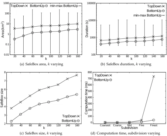
Figure 6: Results with MilanoByNight dataset

In Figure 6(a) we compare the average size of the spatial areas of the SafeBoxes returned byTopDownandBottomUpfor different values ofk. As expected, by increasing the value of

k, slightly larger areas are returned by both algorithms. The comparison between the two algorithms shows that on average theBottomUp algorithm produces much smaller areas (up to an order of magnitude) with respect to theTopDownalgorithm. A similar result is shown in Figure 6(b), in which the duration of the SafeBoxes is compared.

In Figure 6(a), the bars represent the maximum and the minimum size of the areas re-turned byBottomUp. The area’s variance for theTopDownalgorithm is not reported since it is small compared toBottomUpone. The reason of a high variance for BottomUp can find an explanation in the generalization strategy used by the algorithm. Indeed, the algo-rithm takes decisions based on local conditions starting from the leaf nodes. A non-uniform distribution of objects in the considered space leads to significantly different decisions de-pending on the position of the source point leading to significantly different generaliza-tions.

The overall precision, in both time and space, is summarized in Figure 6(c) that compares

of a SafeBox is the level of the SafeBox in the generalization tree described in Section 4.1. This implies that lower is the value, the smaller is the SafeBox in both time and space, and hence the higher is the precision. Figure 6(c) confirms the experimental results of area and duration comparisons: theBottomUpalgorithm produces smaller SafeBoxes up to3levels in the generalization tree, meaning that aTopDownSafeBox can be23

= 8times bigger than aBottomUpSafeBox.

Figure 6(d) shows how the subdivision impacts on the performance of both algorithms. We can observe that the execution time ofBottomUpalgorithm is only slightly affected by the increase of the number of leaf ST-cells, while theTopDownperformance is quite related with it. The execution time is under100milliseconds in the coarsest subdivision and more than700milliseconds in the finest subdivision: this last value can be incompatible with a service that needs to return SafeBoxes in real time.

5.3.2 Evaluation with Google shop dataset with appearance semantics

The second set of experiments tests the two algorithms precision and performance with the Google shops dataset with appearance semantics.

1 2 3 4 5 6

2 4 6 8 10 12 14 16

S

af

eB

ox

si

ze

k

TopDown BottomUp

(a) SafeBox size,k_varying

0 5 10 15 20 25 30

Coarsest Coarse Mid Fine Finest

C

om

pu

ta

tio

n

tim

e

(m

s)

Subdivision TopDown

BottomUp

(b) Computation time, subdivision varying

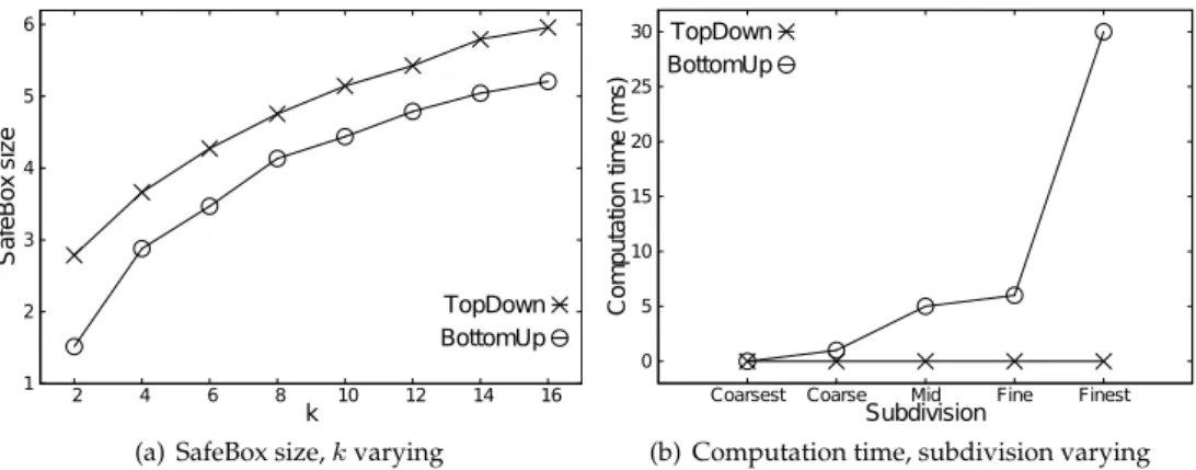
Figure 7: Results with Google Shops dataset - Appearance semantics

Figure 7(a) shows the size of the SafeBoxes returned byTopDownand BottomUp. By in-creasing the value ofk, larger areas are returned by both algorithms. The SafeBox returned byBottomUpis on average smaller in size than the one returned byTopDown, as shown in Figure 7(a). Therefore, we can conclude that theBottomUpalgorithm is preferable since it produces on average smaller SafeBox.

Comparing this result with the one of the MilanoByNight dataset we can observe that the average size of SafeBoxes returned byTopDownwith the Google shops dataset is smaller in comparison with the one returned with MilanoByNight; conversely the average size of SafeBoxes returned byBottomUpis quite the same. The reason is that the distribution of users is less uniform than the distribution of the shops and this negatively affects the per-formance ofTopDown. Vice versaBottomUpis not significantly affected by the distribution of the objects in the space.

subdivisionBottomUptakes up to 30 milliseconds. The difference with respect to the Mi-lanoByNight dataset is due to the different implementation of theΩfunction. In the Google shops setting,TopDownperforms better since the computation ofΩ()is very efficient, while inBottomUpthe computation time is affected by the computation of theResidualsfunction. In any case, the computation time, even with theBottomUpalgorithm, is less than30 mil-liseconds, hence granting a quick response time.

5.3.3 Evaluation with Google shop dataset with persistence semantics

2 3 4 5

5 15 30

S af eB ox si ze D (min) TopDown BottomUp

(a) SafeBox size,D_varying

0 0.5 1 1.5 2 2.5 3

5 15 30

C om pu ta tio n tim e (m s) D (min) TopDown BottomUp

(b) Computation time,D_varying

0 1 2 3 4 5 6

2 4 6 8 10 12 14 16

S af eB ox si ze k

TopDown, D =5 min TopDown, D =15 min TopDown, D =30 min

(c) TopDownSafeBox size,k_varying

0 1 2 3 4 5 6

2 4 6 8 10 12 14 16

S af eB ox si ze k

BottomUp, D =5 min BottomUp, D =15 min BottomUp, D =30 min

(d)BottomUpSafeBox size,k_varying

Figure 8: Results with Google Shops dataset - Persistence semantics

This set of experiments evaluates the two algorithms precision and performance with the Google shops dataset adopting the persistence semantics. Figure 8(a) shows the average SafeBox size ofTopDownandBottomUpalgorithms when varying the persistence interval durationDfrom5minutes to30minutes. As expected, for shorter intervals the SafeBoxes are smaller, on average. This is due to the fact that, for a given ST-cellc, ifDis short, the objects spatially contained incare more likely to be counted more times in the computation ofΩ(c). Clearly larger values ofΩresult, for both algorithms, in smaller SafeBoxes.

is due to the fact that longer persistence interval duration leads to larger SafeBoxes whose computation withBottomUprequires more iterations of the algorithm and hence an increase in the computation time (affected in particular by theResidualsexecution time).

Figure 8(c) shows the SafeBox size by varyingkwith different value of persistence interval durationDfor theTopDownalgorithm. The average size of the SafeBoxes grows with larger value ofkand longer persistence interval durations, confirming both the results shown in Figure 7(a) and in Figure 8(a). Figure 8(d) shows a similar result forBottomUp.

5.3.4 Evaluation with Google shop dataset, appearance semantics and online retrieval of data

Similarly to Section 5.3.2, in this set of experiments we evaluate the performance of Top-DownandBottomUpalgorithms with the Google Shops dataset adopting the appearance semantics and varyingk. In this set of experiments when data is needed to computeΩwe retrieve it from Google servers through the Google Places API. Clearly, in this set of exper-iments the generalization algorithms need to issue a (possibly large) number of requests and this leads, in some cases, to much longer computations. In this set of experiments we give a limit of one minute for each generalization. If the generalization algorithm does not terminate within this time, the generalization procedure is interrupted and it is considered “timed-out”. 0 20 40 60 80 100

2 8 16

C om pu ta tio n tim e > 1 m in (% ) k TopDown BottomUp

(a) Percentage of failed experiments,k_varying

0 5 10 15 20 25 30 35 40 45 50 55

2 8 16

C om pu ta tio n tim e (s ) k TopDown BottomUp

(b) Computation time,k_varying

0 50 100 150 200 250 300

2 8 16

# of re tr ie ve d pl ac es k TopDown BottomUp

(c) Number of Places,k_varying

Figure 9(a) shows the percentage of runs that were timed-out for our proposed algorithms. We can observe that fork= 2this percentage is of about2% and6%, forBottomUpand Top-Down, respectively. When increasing the value ofkup to16the percentage grows, since both algorithms need to retrieve more points (see Figure 9(c)). However, while with Top-Downmore than60% of the generalization runs are timed out withk= 16, withBottomUp

the percentage is much smaller (i.e., less than10%).

Figure 9(b) shows the average computation time computed among the runs that were not timed-out. We can observe thatTopDownhas a much larger computation time than

BottomUpfor different values ofk. The main reason for this result is thatBottomUprequires to retrieve less points. Indeed in Figure 9(c) we can observe that, for all considered values ofk,BottomUprequires about one fifth of the points that are needed byTopDown.

5.3.5 Comparison with Grid algorithm

0.01 0.1 1 10

20 40 60 80 100 120 140 160

A

re

a

(k

m

^2

)

k

TopDown BottomUp Grid

(a) SafeBox size,k_varying

0 10 20 30 40 50 60 70

20 40 60 80 100 120 140 160

tim

e

(m

s)

k

TopDown BottomUp Grid

(b) Computation time,k_varying

Figure 10: Comparison with existing solutions

In this last set of experiments we compare theTopDownandBottomUp algorithms with theGridspatial generalization algorithm, presented in [12]. These experiments have been run with the MilanoByNight dataset adopting the appearance semantics. As in the previ-ous experiments, the spatial domainS is Milano’s area, but the temporal domain consists in only a screenshot of MilanoByNight’s temporal duration, since theGridalgorithm pro-vides only a spatial generalization. We briefly recall thatGridalgorithm adopts a top-down strategy, in which a total order on the data (e.g., users’ locations) needs to be established for computing the generalized area.

In Figure 10(a) we can observe, for different values ofk, that Gridreturns, on average, smaller areas and hence can provide a higher data utility. However Figure 10(b) shows thatGridhas a much higher computation time.