Dual-force ISOMAP: a new relevance feedback method for medical image retrieval.

(1)

for Medical Image Retrieval

Hualei Shen1,3, Dacheng Tao2*, Dianfu Ma1*

1State Key Laboratory of Software Development Environment, School of Computer Science and Engineering, Beihang University, Beijing, China,2Center for Quantum Computation and Intelligent Systems, Faculty of Engineering and Information Technology, University of Technology, Sydney, NSW, Australia,3School of Computer and Information Engineering, Henan Normal University, Xinxiang, China

Abstract

With great potential for assisting radiological image interpretation and decision making, content-based image retrieval in the medical domain has become a hot topic in recent years. Many methods to enhance the performance of content-based medical image retrieval have been proposed, among which the relevance feedback (RF) scheme is one of the most promising. Given user feedback information, RF algorithms interactively learn a user’s preferences to bridge the ‘‘semantic gap’’ between low-level computerized visual features and high-level human semantic perception and thus improve retrieval performance. However, most existing RF algorithms perform in the original high-dimensional feature space and ignore the manifold structure of the low-level visual features of images. In this paper, we propose a new method, termed dual-force ISOMAP (DFISOMAP), for content-based medical image retrieval. Under the assumption that medical images lie on a low-dimensional manifold embedded in a high-low-dimensional ambient space, DFISOMAP operates in the following three stages. First, the geometric structure of positive examples in the learned low-dimensional embedding is preserved according to the isometric feature mapping (ISOMAP) criterion. To precisely model the geometric structure, a reconstruction error constraint is also added. Second, the average distance between positive and negative examples is maximized to separate them; this margin maximization acts as a force that pushes negative examples far away from positive examples. Finally, the similarity propagation technique is utilized to provide negative examples with another force that will pull them back into the negative sample set. We evaluate the proposed method on a subset of the IRMA medical image dataset with a RF-based medical image retrieval framework. Experimental results show that DFISOMAP outperforms popular approaches for content-based medical image retrieval in terms of accuracy and stability.

Citation:Shen H, Tao D, Ma D (2013) Dual-Force ISOMAP: A New Relevance Feedback Method for Medical Image Retrieval. PLoS ONE 8(12): e84096. doi:10.1371/ journal.pone.0084096

Editor:Xi-Nian Zuo, Institute of Psychology, Chinese Academy of Sciences, China ReceivedJuly 19, 2013;AcceptedNovember 12, 2013;PublishedDecember 31, 2013

Copyright:ß2013 Shen et al. This is an open-access article distributed under the terms of the Creative Commons Attribution License, which permits unrestricted use, distribution, and reproduction in any medium, provided the original author and source are credited.

Funding:This work was supported in part by the following projects: 1. National Natural Science Foundation of China under grant number 61003017, 2. Project of State Key Laboratory of Software Development Environment under grant number SKLSDE-2013ZX-30, 3. ARC Discovery Project under grant number DP140102164. The funders had no role in study design, data collection and analysis, decision to publish, or preparation of the manuscript.

Competing Interests:The authors have declared that no competing interests exist. * E-mail: dacheng.tao@uts.edu.au (DCT); dfma@buaa.edu.cn (DFM)

Introduction

Medical image interpretation is a process which incorporates subjective perception and objective reasoning. Typically, radiol-ogists obtain superficial visual features from medical images and render diagnostic conclusions based on personal knowledge and experience. Due to differences of perception, training and fatigue, different conclusions about the same medical image will be drawn by different professionals or by the same professional under different circumstances [1,2]. The goal of content-based medical image retrieval (CBMIR) is to enable radiologists to make better diagnosis about a given case by retrieving similar cases from a variety of semantically annotated medical image archives.

It is well-known that ‘‘semantic gap’’ is one of the issues faced by content-based image retrieval (CBIR). The fact that medical images contain varied, rich and subtle visual features [3] is an additional challenge to the use of CBIR in radiology. Unlike from regular image understanding, medical image diagnosis is depen-dent on case-specific interpretation. It is common for visually similar medical images to convey different semantic meanings, while semantically-alike images have different visual features. Let

us take medical images obtained from IRMA medical image dataset [4] as an example. The IRMA medical image dataset is a widely used test bed for performance evaluation of CBMIR [5–8]. The new version of IRMA dataset [4] contains 12,677 fully annotated gray value radiographs in a training set. These images are categorized into 193 classes according to a mono-hierarchical multi-axial classification standard called the IRMA coding system [9]. The system classifies a medical image from four orthogonal axes: imaging modality, body orientation, body region examined and biological system examined.Figure 1andFigure 2illustrate the scenario of semantic gap. As shown inFigure 1, two chest radiographs have a similar visual appearance, but their semantic meanings are different. The IRMA code [9] of the left image is ‘‘1123-127-500-000’’, while the IRMA code of the right image is ‘‘1123-110-500-003’’. By contrast, though their visual appearance is different, the two mammograms shown inFigure 2have the same IRMA code ‘‘1124-310-610-625’’.

(2)

retrieval system to refine the retrieval results. The basic process of RF in CBIR is as follows: 1) the retrieval system returns the initial retrieval results to the user; 2) the user labels query-relevant images and query-irrelevant images as positive feedback and negative feedback, respectively; 3) based on the labeled feedback, the retrieval system learns to improve the retrieval performance and returns new results; 4) if the user is satisfied with the new results, the RF process ends; otherwise, go to 2).

Over the past decades, many representative RF approaches have been proposed in the context of CBIR [13–23]. A comprehensive survey of these methods can be found in [11,24]. In [25], RF methods are categorized into four groups: subspace selection-based schemes, support vector machine (SVM)-based schemes, random sampling-based schemes and feature reweight-ing-based schemes. Performance evaluations of several RF approaches are reported in [26,27].

Many RF methods have also appeared in CBMIR in recent years. Rahman et al. [28] utilized positive feedback to update the optimal query point for medical image retrieval. They proposed a RF-based dynamic similarity fusion approach for biomedical image retrieval [29] in which RF information is utilized to reweight features at each iteration. Xu et al. [30,31] utilized RF to update feature weights for X-ray image retrieval. To solve the small sample size problem, Hoi et al. [32] proposed a method called semi-supervised SVM batch mode active learning for both medical and regular image retrieval. In addition, Ko et al. [33] integrated the RF scheme into CBMIR to boost retrieval performance. Though the approaches mentioned above achieve promising results, there is room for performance enhancement because most of these methods do not consider the manifold structure of low-level image features.

In this paper, we formulate a new RF method termed dual-force ISOMAP (DFISOMAP) for CBMIR. DFISOMAP is proposed in the context of precisely exploring the manifold structure of low-level image visual features [34–36]. DFISOMAP operates in the following three stages: 1) the local geometry preservation stage, 2) the margin maximization stage, and 3) the similarity propagation stage. First, the local geometry of the positive examples in the high-dimensional feature space is preserved according to the isometric feature mapping (ISOMAP) criterion [37]. To precisely model the geometric structure of positive examples in the low-dimensional embedding, a reconstruction error constraint accord-ing to locally linear embeddaccord-ing (LLE) [38] is also added. Second, negative examples are pushed away from positive examples by a force driven by the maximization of average pairwise distances between the positive and negative examples. Finally, negative examples are pulled into the negative sample set by another force

generated by similarity propagation. We conduct experiments to demonstrate the effectiveness of DFISOMAP. Compared to conventional RF methods, e.g., linear discriminant analysis (LDA) [39], locality preserving projections (LPP) [40], biased discriminant analysis (BDA) [21], constrained similarity measure using support vector machine (CSVM) [18], ISOMAP and exponential locality preserving projections (ELPP) [41], DFISO-MAP differ in the following ways: 1) DFISODFISO-MAP precisely preserves the geometric structure of positive feedback examples, and 2) DFISOMAP does not suffer from the undersampling problem.

Dual-Force ISOMAP

In this section, we detail the proposed DFISOMAP. To better present the method,Table 1lists important notations used in this paper.

Consider a set of medical imagesI~_½~_x_x₁, ,~xxN[Rh|N in low-level feature space, and a query image~xxq[I:Following the query-by-example paradigm of the CBIR system, there are top n

returned images for each query, from which we obtainnzimages

which are from the same semantic class as~xxq: We term them positive examples:~xxq1, ,~xxqnz:Putting these examples together, we get apositive feedback setXz~½~xx_q1, ,~xxqnz:Meanwhile, we obtain n{ images, which are from different semantic classes with respect

to~xxq:We term themnegative examples:~xxq1, ,~xxqn{:Putting these examples together, we get a negative feedback set

X{~½~xxq1, ,~xxqn{:The relevance feedback setX is constructed by putting ~xxq1, ,~xxqnz and ~xxq

1, ,~xxqn{ together as X~_½~_x_xq1, ,~xxqnz,~xxq

1, ,~xxqn{: where the first nz are positive examples and the remaining n{ are negative examples,

nzzn{~n: For convenience, we use~xxi(1ƒiƒn) to represent

all examples, and denoteX~_½~xx1, ,~xxn,Xz~½~xx1, ,~xxnz,and X{~½~xx1znz, ,~xxn{znz:

DFISOMAP assumes that medical images lie on a low-dimensional manifold Rl and are artificially embedded in a high-dimensional ambient space, i.e., the low-level feature space Rh:The objective of DFISOMAP is to learn a mapping functionF

from Rh to Rl, based on the relevance feedback set X: The learned mappingF should effectively separate positive examples from negative examples. For simplicity, we assume thatFis linear. The problem of DFISOMAP is then converted to find a projection

Figure 1. Visually similar medical images contain different semantic meanings.The chest radiographs shown in this figure have a similar visual appearance but belong to different semantic categories. Images are taken from IRMA medical image dataset.

doi:10.1371/journal.pone.0084096.g001

(3)

matrixU[Rh|lthat mapsX[RhtoY[Rl,i.e.,Y~UT_X_,_where l%h:Here, each column ofYis~yyi~UT_~_x_xi_:

DFISOMAP operates in three stages which containing two forces to separate negative examples from positive examples. In the first stage, the local geometric structure of the positive examples is preserved according to the ISOMAP criterion [37]. To make the local geometry preservation more precise, an error reconstruction constraint is added. This stage is termed ‘‘local geometry preservation’’. In the second stage, a margin maximization function is defined to maximize the gap between positive examples and negative examples. The margin maximization function acts as a force to push negative examples away from positive examples, and this stage is termed ‘‘margin maximization’’. In the final stage, termed ‘‘similarity propagation’’, the similarity propagation technique [42] is employed to build a similarity matrix which quantifies similarities between the intraclass examples contained in the relevance feedback set. Based on the similarity matrix, the distance between the intraclass examples is minimized to shrink the distance between image pairs from the same semantic class. The procedure acts as another force to pull negative examples away from positive examples.

2.1. Local Geometry Preservation

ISOMAP preserves the local geometry of positive examples by the following objective function [37]

arg min

~y_yi,1ƒiƒnz

X nz

i~1 X

nz

j~1

(dG(~xxi,~xxj){dE(~yyi,~yyj))2, ð1Þ

wheredG(~xxi,~xxj)is the geodesic distance between image~xxiand~xxj

in high-dimensional spaceRh:AnddE(~yyi,~yyj)is the corresponding Euclidean distance between image~xxiand~xxjin low-dimensional embeddingRl,~yyi~UT_~_xi_x_,_~_y_yj_~_UT_~_x_xj_:

Let us denote½DG_ij~dG(~xxi,~xxj), ½DE_ij~dE(~yyi,~yyj):Where DG

andDEarenz|nzmatrices. According to [37],DGandDEcan be

converted to inner product matrixt(DG) andt(DE),respectively. Operatort(D)is defined as

t(D)~{1

2HDDH~ , ð2Þ

H~Inz{

1

nz

~eenz~ee

T

nz, ð3Þ

½DD~_i_,_j~½D2_i_,_j: ð4Þ

whereInz is annz|nz identity matrix,~eenz~(1,. . .,1) T_[

Rnz : Thus, equation (1) can be transformed to

arg min

~y_yi,1ƒiƒnz

X nz

i~1 X

nz

j~1

(dG(~xxi,~xxj){dE(~yyi,~yyj))2

~ arg min

~y_yi,1ƒiƒnz

t(DG){t(DE)

k k2

~arg min

Yz

t(DG){YzTYz

2

~arg min

Yz

tr½t(DG)t(DG)T{2Yzt(DG)YzTzY

T

zYY

T

zY,

ð5Þ

wheretr½.stands for the trace operator,Yz~UTXz:Assuming

thatYT

zY is a constant matrix, equation (5) can be converted to

Table 1.Important notations used in this paper.

Notation Description Notation Description

I medical image dataset N _{similarity matrix}

Rh _{high-dimensional ambient space} _~_x_x_i _the_i_th_{medical image contained in}_X

Rl low-dimensional embedding ~yyi theithmedical image contained inY

X relevance feedback set inRh _d_G₍_~_x_x_i_,_~_x_x_j₎ _{geodesic distance between}_~_x_x_i_and_~_x_x_j Xz positive relevance feedback set dE(~yyi,~yyj) Euclidean distance between~yyiand~yyj

X{ negative relevance feedback set nz size ofXz

Y relevance feedback set inRl n{ size ofX{

U projection matrix,Y~UT_X _~_ee _{identity vector}

I identity matrix a trade-off parameter

W reconstruction coefficient matrix in LLE b trade-off parameter

t(D) linear product matrix ofD c margin factor

(4)

arg min

~y_yi,1ƒiƒnz

X nz

i~1 X

nz

j~1

(dG(~xxi,~xxj){dE(~yyi,~yyj))2

~arg min

Yz

tr½{2Yzt(DG)YzT

~arg max

U

tr½UTXzt(DG)XzTU

~arg max

U

tr½UTAU,

ð6Þ

whereA~Xzt(DG)XzT:

To minimize reconstruction error of the local geometry preservation presented above, we further assume each ~yyi[Y_z can be reconstructed by its neighbors. Thus, we have

arg min

~y_yi,1ƒiƒnz

X nz

i~1

~yyi{ X

1ƒjƒnz,j=i

Wi,j~yyj

2

~arg min

Yz

tr½Yz(I{WT)(I{WT)TYzT

~arg min

U

tr½UTXz(I{WT)(I{WT)TXzTU

~arg min

U

tr½UTBU,

ð7Þ

where B~Xz(I{WT)(I{WT)TXzT,I is annz|nz identity

matrix.Wi,jis obtained via locally linear embedding (LLE) [38]: Figure 3. Relevance feedback-based medical image retrieval framework.

Figure 4. Examples of images in IRMA medical image testbed.

Figure 5. Examples of query image.

(5)

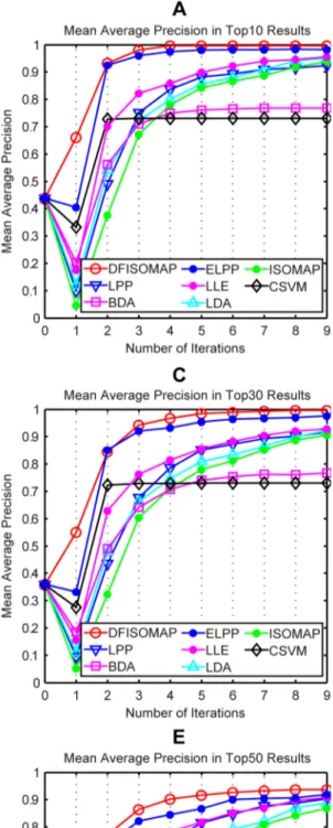
Figure 6. MAP values of DFISOMAP, LPP, BDA, ELPP, LLE, LDA, ISOMAP and CSVM.Subfigures (A), (B), (C), (D) and (E) detail MAP values in the top 10, top 20, top 30, top 40 and top 50 results, respectively.

(6)

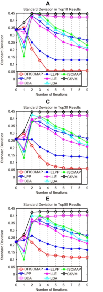
Figure 7. SD values of DFISOMAP, LPP, BDA, ELPP, LLE, LDA, ISOMAP and CSVM.Subfigures (A), (B), (C), (D) and (E) detail SD values in the top 10, top 20, top 30, top 40 and top 50 results, respectively.

(7)

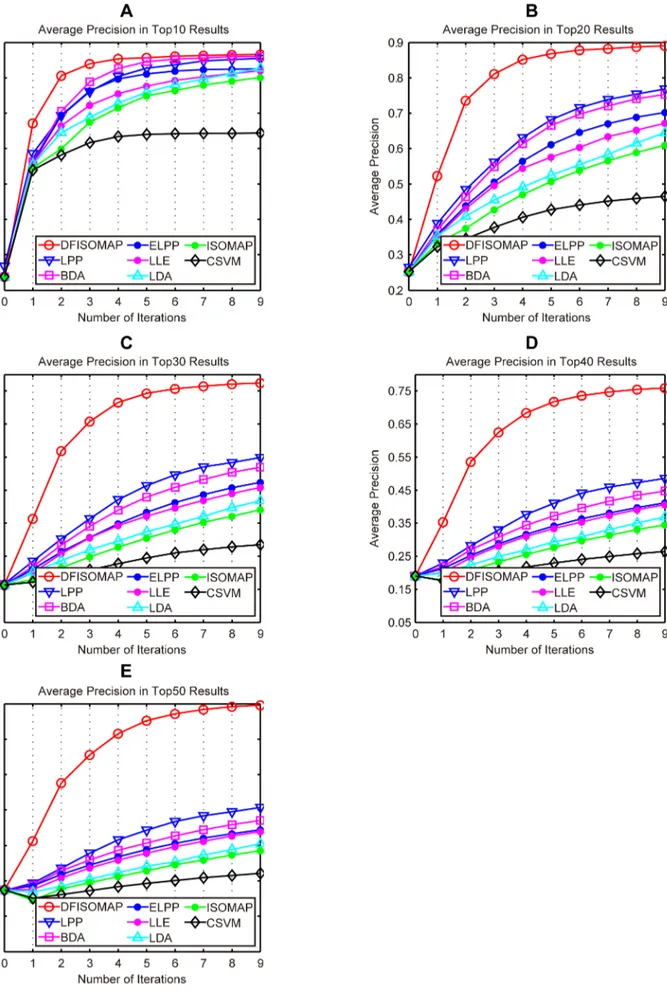
Figure 8. AP of DFISOMAP, LPP, BDA, ELPP, LLE, LDA, ISOMAP and CSVM.Subfigures (A), (B), (C), (D) and (E) detail AP in the top 10, 20, 30, 40, and 50 results, respectively.

(8)

Wi,j~ arg minWi,j P nz

i~1

~xxi{ P 1ƒjƒnz,j=i

Wi,j~xxj 2 ,P

jWi,j~1,i=j

0,i~j

: 8 > < > : ð8Þ

Putting equation (6) and (7) together, we obtain the objective function for local geometry preservation

arg max

U

tr½UT(A{aB)U, ð9Þ

wherea§0is the trade-off parameter.

2.2. Margin Maximization

In the low-dimensional embedding, we expect that the average pairwise distances between negative and positive feedback examples will be as large as possible, and the average pairwise distances among positive feedback examples will be as small as possible, i.e.,

arg max

~y_yk,1ƒkƒn

1

nz|n{

X nz

i~1 X n{ znz

j~1znz

~yyi{_~yyj 2 { h nz|nz

X nz

i~1 X

nz

j~1

~yyi{_~yyj 2 : ð10Þ

Whereh§1is the gap factor. Considering~yyi~UT_~_x_xi_,_equation

(10) reduces to:

arg max

~y_yk,1ƒkƒn

1

nz|n{

X nz

i~1 X n{ znz

j~1znz

~yyi{_~yyj 2 { h nz|nz

X nz

i~1 X

nz

j~1

~yyi{_~yyj

2

~arg max

U

1

nz|n{

X

~x_xi[Xz

X

~ x xj[X{

UT_(~_x_xi_{_~_x_xj₎ 2 { h nz|nz

X

~x_xi[Xz

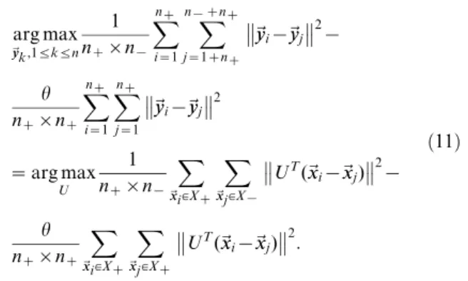
X

~ x xj[Xz

UT(~xxi{_~xxj) 2 : ð11Þ

2.3. Similarity Propagation

Equation (11) only takes into account the distances between the positive examples and coarsely treats negative examples. To remedy this, we need the average pairwise distance among the intraclass examples to be rendered as small as possible.

The straightforward way to shrink the pairwise distance between interclass examples is to minimize the average weighted square distance between all sample pairs(~yyi,~yyj),0ƒi,jƒn,in the low-dimensional embedding:

arg min

Y

1

n|n Xn

i~1 Xn

j~1

~yyi{~yyj

2

Ni,j

~arg min

U

1

n|n Xn

i~1 Xn

j~1

UT_(~_x_xi_{_~_x_xj₎

2

N_i_,_j

~arg min

U

1

n|n X

~x_xi[X X

~ x xj[X

2

N_i_,_j,

ð12Þ

whereN[Rn|n_{is termed similarity matrix.} In this paper, we defineN_as

Table 2.Average precision of top ranked results for different methods after fifth feedback.

Methods top10 top20 top30 top40 top50

DFISOMAP 0.9571 0.8676 0.7931 0.7180 0.6530

LPP 0.9270 0.6818 0.5138 0.4107 0.3435 BDA 0.9459 0.6652 0.4785 0.3726 0.3067 ELPP 0.9112 0.6120 0.4332 0.3629 0.3054 LLE 0.8766 0.5757 0.4211 0.3341 0.2782 LDA 0.8586 0.5253 0.3742 0.2937 0.2420 ISOMAP 0.8491 0.5064 0.3548 0.2763 0.2285 CSVM 0.7396 0.4269 0.2951 0.2290 0.1926

doi:10.1371/journal.pone.0084096.t002

Table 3.Average precision of top ranked results for different methods after ninth feedback.

DFISOMAP 0.9660 0.8901 0.8246 0.7587 0.6965

(9)

Figure 9. AR of DFISOMAP, LPP, BDA, ELPP, LLE, LDA, ISOMAP and CSVM.Subfigures (A), (B), (C), (D) and (E) detail AR in the top 10, 20, 30, 40, and 50 results, respectively.

(10)

N~ exp ({ ~xxi{_~xxj

2

2t2 ),if~xxi,~xxj[Xzor~xxi,~xxj[X{

0,otherwise : 8 < : ð13Þ

N_{quantifies the similarity relationship among positive and}

negative examples, respectively. In our implementation, we settas 0.5.

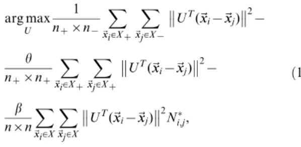
Putting equation (11) and (12) together, we have

arg max

U

1

nz|n{

X

~x_xi[Xz

X

~x_xj[X{

UT_(~_x_xi_{_~_x_xj₎ 2 { h nz|nz

X

~x_xi[Xz

X

~x_xj[Xz

UT(~xxi{_~xxj) 2 { b n|n

X

~x_xi[X X

~x_xj[X

UT(~xxi{_~xxj)

2

N_i_,_j,

ð14Þ

wherebw0is the trade-off parameter. Let us denote

Mi,j~

{ b

n|nN

i,j{ h

nz|nz

, if 1ƒiƒnz,1ƒjƒnz

{ b

n|nN

i,jz

1 nz|n{

,if 1ƒiƒnz,1znzƒjƒn{znzor 1znzƒiƒn{znz,1ƒjƒ1znz

{ b

n|nN

i,j,others

8 > > > > > > > < > > > > > > > : :ð15Þ

Then equation (14) can be rewritten as

arg max

U

1

nz|n{

X

~x_xi[Xz

X

~x_xj[X{

UT(~xxi{_~xxj) 2 { h nz|nz

X

~x_xi[Xz

X

~x_xj[Xz

UT_(~_x_xi_{_~_x_xj₎ 2 { b n|n

X

~x_xi[X X

~x_xj[X

UT(~xxi{~xxj)

2

Ni,j

~arg max

U Xn

i~1 Xn

j~1

2

Mi,j

~arg max

U

2tr½UTX(L{M)XTU

~arg max 2

U

tr½UTCU

~arg max

U

tr½UTCU,

ð16Þ

whereC~X(L{M)XT_,_L_{is a diagonal matrix,}_Li

,i~Pnj~1Mi,j:

Combining equation (9) with (16), we obtain the objective function of DFISOMAP

arg max

U

tr½UT₍_A_{_a_B₎_U_z_c_tr_½_UT_CU

~arg max

U

tr½UT₍_A_{_a_B_z_c_C₎_U

~arg max

U

tr½UT_EU_,

ð17Þ

wherec§0is the margin factor,E~A{aBzcC:

Because the real matrixE is symmetric (the proof is given in Appendix S1),U can be solved by standard eigenvalue decom-position onE:By imposingUUT_~_Il_{on (17),}_U_{is formed by the}_l

eigenvectors associated with the firstllargest eigenvalues.

CBMIR Framework

We utilize the framework depicted in Figure 3for CBMIR. Any RF feedback algorithm can be integrated into this framework. As shown in this figure, when a query image is provided, its low-level visual features are extracted. All images contained in the medical image database are then sorted in ascending order according to their distance from the query image measured by Euclidean metric. If the user is not satisfied with the result, s/he labels some semantically relevant images as positive feedback examples and some semantically irrelevant images as negative feedback examples. Based on these feedback examples, a RF model can be trained. All images, including the positive feedback, the negative feedback and the remaining images contained in the medical image database, are re-sorted based on the updated similarity metric and the top-ranked images are returned. If the user is not satisfied with the result, the RF process is repeated.

For DFISOMAP, we learn a projection matrixU according to equation(17). Then we useU to project all the images to the low-dimensional embedding. In the projected embedding, each image is re-sorted in ascending order with respect to its Euclidean distance from the query image and the top-ranked images are returned to the user. The RF procedure stops when the user is satisfied with the results.

We use LBP [43], SIFT [44] and pixel intensity descriptors respectively to extract features from the medical image. For the

Table 4.Average recall of top ranked results for different methods after fifth feedback.

DFISOMAP 0.0985 0.1758 0.2351 0.2746 0.3025

(11)

LBP descriptor, we divide each medical image into 363 equal

regions. On each region, a 59-bin LBP histogram is built. Then we concatenate these 59-bin LBP histograms into a 531-D vector. For the SIFT and intensity descriptors, we follow bag of features [45] scheme to represent the image. In detail, we first densely sample each image with SIFT and the intensity descriptor, respectively. We set the sampling space as 8, and the patch size as 16616. Then

we use K-means clustering to learn two 500-word dictionaries, i.e., SIFT and intensity visual word dictionary. Finally, for each image, we obtain a 500-bin SIFT and intensity histogram, respectively.

We represent each image by concatenating the 531-bin LBP histogram, 500-bin SIFT histogram and 500-bin pixel intensity histogram into a 1531-D long vector. To get rid of redundant information contained in the concatenated vector and reduce the computational complexity in the next section, we normalize the concatenated 1531-D vector into a normal distribution with zero mean and one standard deviation. Then we use principal component analysis (PCA) to reduce the normalized vector to a 500-D feature vector.

Performance Evaluation

In this section, we report performance of the proposed DFISOMAP for CBMIR comparing with that of other methods, i.e., LDA, LPP, BDA, CSVM, ISOMAP, LLE and ELPP.

This section is organized as follows. In section 4.1, we introduce the dataset used for evaluation. Section 4.2 presents experimental setup. In section 4.3, we compare DFISOMAP with other RF approaches using mean average precision (MAP) and standard deviation (SD). Section 4.4 reports performance evaluation results of RF methods in terms of precision and recall. Finally, we explore effects of parameters on the performance of DFISOMAP in section 4.5.

4.1. IRMA Medical Image Dataset

The IRMA medical image dataset is widely used for CBMIR evaluation. In our experiment, we select the first 57 categories from the new version of IRMA dataset as test bed. The selected images contain a total of 10,902 images.Figure 4shows example images from the dataset.Figure 5illustrates three query images.

4.2. Experimental Setting

We conduct 338 independent experiments to evaluate perfor-mance of DFISOMAP and other RF methods. In detail, we randomly select 338 images from the IRMA data set as query examples. These images belong to different IRMA categories. In general, five or six images are selected from each IRMA category. In initial retrieval, for each query sample, there are five to eight relevant images in top30 ranked results. For each selected image, a ‘‘leave one out’’ query is conducted: Rest images contained in the data set are ranked according to their Euclidean distance to the query sample.

Different RF algorithms are embedded into the framework depicted inFigure 3. The RF process is automatically performed by the computer. A computer-simulated query for each query image is performed on all the other 10,901 images contained in the dataset. The computer marks all query relevant images as positive feedback in the top 30 images and the rest as negative feedback. In general, we have between two and eight images as positive feedback. The procedure is close to a real-world application scenario, because typically the user does not want to label many feedback examples in the iteration process. We set the number of RF iterations as 10. For the first iteration, the returned images are ranked according to their Euclidean distance from the query

image. Starting from the second iteration, different RF algorithms learn different projection matrices U based on positive and negative feedback, respectively. In the projected low-dimensional embedding, other images in the dataset are re-ranked according to their Euclidean distance from the query image.

We parameterize the settings of all baseline methods according to the descriptions in corresponding papers. In the experiments, the parameters of different methods are tuned to obtain the best results. For CSVM, we choose the Gaussian kernel

K(~xxi,~xxj)~exp ({s~xxi{_~xxj

2

) with s~_0:5: LibSVM [9] is utilized to achieve an optimal hyperplane to separate negative and positive examples. For ELPP, we set parameters as what is described in [41].

4.3. Performance Evaluation Using MAP and SD

In this section, we use MAP and SD to measure the performance of DFISOMAP and other RF algorithms. MAP is the mean of average precision values of the 338 independent queries. MAP value measures the retrieval precision of RF algorithms. SD value is computed from AP values of the 338 independent queries. SD value assesses the stability of RF algorithms.

Figure 6andFigure 7illustrate performance of the proposed DFISOMAP compared to LDA, LPP, BDA, CSVM, ISOMAP, LLE and ELPP-based RF algorithms. InFigure 6, subfigures (A), (B), (C), (D) and (E) show MAP values for the top 10, 20, 30, 40 and 50 results, respectively. The eight curves in each of these subfigures illustrate performance of the RF algorithms. The x-coordinate represents number of iterations, which varies from 0 to 9. Iteration 0 represents the initial retrieval measured by Euclidean distance in the high-dimensional feature space without RF, while iteration 1 refers to the first round RF based on feedback examples labeled in the 0th iteration, and similarly other iterations (from iteration 2 to 9). The y-coordinate indicates MAP values of different RF algorithms after each iteration. In Figure 7, subfigures (A), (B), (C), (D) and (E) detail SD values in the top 10, 20, 30, 40 and 50 results, respectively. SD indicates stability of the RF algorithm: the smaller the SD value, the more stable the algorithm.

From the figure we can see that, in all experiments, and after any number of iterations, the proposed DFISOMAP consistently outperforms other conventional RF algorithms in terms of MAP. The DFISOMAP also shows good stability, as demonstrated by the SD value and tendency of the SD curve. At each level (top 10

Table 5.Average recall of top ranked results for different methods after ninth feedback.

DFISOMAP 0.0993 0.1810 0.2464 0.2931 0.3253

(12)

to 50), it can be seen that SD values of DFISOMAP for further iterations decrease after one iteration, and are much lower than those of other RF algorithms.

4.4. Performance Evaluation Using Precision and Recall In this section, we utilize average precision (AP) and average recall (AR) to evaluate performance of DFISOMAP and other methods. In the context of CBMIR, precision refers to percentage of relevant medical images in top retrieved results. AP is calculated as the averaged precision values obtained via all queries. And recall refers to percentage of relevant medical images in all relevant examples contained in the test bed. AR is averaged recall values of all queries.

Figure 8,Table 2andTable 3show AP of different methods. In detail,Figure 8(A), (B), (C), (D) and (E) present AP of different methods in the top 10, 20, 30, 40, and 50 results, respectively. As we can see from the figure, it is evident that DFISOMAP subsequently outperforms other algorithms. Details of the AP values of top ranked results for different approaches after the fifth and ninth feedback are presented in Table 2 and Table 3, respectively. From these two tables, we can draw the conclusion that DFISOMAP achieves more promising results compared with other methods.

Figure 9, Table 4 and Table 5 present AR of different algorithms. Specifically, Figure 9 (A), (B), (C), (D) and (E) demonstrate AR of different approaches obtained in the top 10, 20, 30, 40, and 50 results, respectively. We can conclude from the figure that DFISOMAP is more effective than the other compared methods. Moreover, AR values of top ranked results for different methods after the fifth and ninth feedback are given inTable 4

andTable 5, respectively. According to these two tables, we can see that DFISOMAP is more effective than other approaches.

4.5. Effects of Parameters

(1) Effects of a. As shown in equation (17), parame-teracontrols the contribution ofBtoE:WhereBstands for utilizing LLE to preserve local geometry of positive feedback examples.

With the same experimental setup detailed above, we conduct experiments to evaluate effects of a:In our experiments, we increaseafrom 0 to 100 with step 10, and setcas 1400.Table 6

andTable 7show AP and AR of DFISOMAP in top50 results, respectively. From which we can draw the following conclusions. 1) DFISOMAP achieves best performance whenais set as 10. 2) With the increasing ofa,performance of DFISOMAP degrades. 3) Whenais set as 0, i.e.,Bhas no contribution toE,performance of DFISOMAP is worst. The conclusion verifies the effectiveness of

iteration 1 2 3 4 5 6 7 8 9

a~0 0.2866 0.4261 0.5004 0.5486 0.5796 0.6043 0.6207 0.6297 0.6369

a~10 0.3124 0.4770 0.5563 0.6164 0.6530 0.6720 0.6839 0.6923 0.6965

a~20 0.3105 0.4759 0.5607 0.6182 0.6488 0.6660 0.6800 0.6870 0.6952

a~30 0.3086 0.4734 0.5617 0.6181 0.6477 0.6660 0.6769 0.6842 0.6886

a~40 0.3072 0.4691 0.5628 0.6204 0.6527 0.6696 0.6796 0.6877 0.6931

a~50 0.3063 0.4670 0.5588 0.6123 0.6442 0.6620 0.6734 0.6821 0.6869

a~60 0.3056 0.4662 0.5557 0.6064 0.6374 0.6543 0.6649 0.6717 0.6766

a~70 0.3047 0.4661 0.5568 0.6091 0.6386 0.6554 0.6689 0.6779 0.6835

a~80 0.3042 0.4639 0.5549 0.6056 0.6358 0.6540 0.6678 0.6775 0.6827

a~90 0.3033 0.4634 0.5549 0.6057 0.6352 0.6521 0.6649 0.6730 0.6782

a~100 0.3026 0.4636 0.5535 0.6073 0.6359 0.6535 0.6658 0.6734 0.6789

Table 7.Average recall of DFISOMAP with differentain top50 results, andaincreases from 0 to 100, with step 10.

iteration 1 2 3 4 5 6 7 8 9

a~0 0.1336 0.1911 0.2244 0.2465 0.2608 0.2727 0.2802 0.2844 0.2879

a~10 0.1467 0.2167 0.2558 0.2850 0.3025 0.3123 0.3186 0.3229 0.3253

a~20 0.1459 0.2161 0.2584 0.2865 0.3018 0.3105 0.3174 0.3212 0.3258

a~30 0.1452 0.2146 0.2585 0.2857 0.3005 0.3104 0.3163 0.3200 0.3222

a~40 0.1447 0.2127 0.2584 0.2870 0.3025 0.3112 0.3167 0.3212 0.3242

a~50 0.1443 0.2121 0.2569 0.2838 0.2992 0.3078 0.3141 0.3192 0.3217

a~60 0.1440 0.2116 0.2552 0.2803 0.2952 0.3033 0.3090 0.3129 0.3155

a~70 0.1437 0.2115 0.2555 0.2819 0.2965 0.3044 0.3112 0.3158 0.3188

a~80 0.1434 0.2108 0.2550 0.2811 0.2962 0.3046 0.3111 0.3162 0.3191

a~90 0.1431 0.2104 0.2551 0.2806 0.2954 0.3032 0.3091 0.3135 0.3163

a~100 0.1428 0.2104 0.2546 0.2810 0.2954 0.3035 0.3095 0.3134 0.3162

(13)

applying LLE to minimize reconstruction error within positive feedback examples.

(2) Effects ofc.Equation (17) demonstrates thatccontrols the contribution ofCtoE:WhereCstands for similarity propagation in positive and negative examples.

With the same experimental setup mentioned above, we conduct experiments to explore effects of c:In our experiments, we increasecfrom 0 to 2000 with step 200, and set as 10.Table 8

andTable 9detail AP and AR of DFISOMAP in top50 results, respectively. From the table we can draw the following conclu-sions. 1) DFISOMAP achieves best performance whencis set as 1400. 2) Whencis set as 0, i.e., there is no similarity propagation, performance of DFISOMAP is worst. The conclusion confirms effectiveness of similarity propagation.

Conclusion

Starting from the assumption that medical images are artificially embedded in a high-dimensional visual feature space, we propose the dual-force ISOMAP (DFISOMAP) to map medical images from high-dimensional feature space to low-dimensional embed-ding. In the framework of CBMIR, DFISOMAP precisely preserves the geometric structure of positive feedback examples

according to the ISOMAP criterion, and effectively separates negative examples from positive examples by utilizing two forces. The evaluation results on a subset of the IRMA medical image dataset show that DFISOMAP outperforms popular dimension-ality reduction-based RF algorithms, e.g., LDA, BDA, LPP, ISOMAP, LLE, ELPP and support vector machine-based RF algorithms, e.g., CSVM.

Supporting Information

Appendix S1 Proof ofEis symmetric. (DOC)

Acknowledgments

We thank Prof. Dr. T. M. Deserno of the Dept. of Medical Informatics, RWTH Aachen, Germany, for providing us with the IRMA medical image dataset. We also thank Mr. Adams Wei Yu at Carnegie Mellon University for his helpful discussions.

Author Contributions

Conceived and designed the experiments: HS DT DM. Performed the experiments: HS. Analyzed the data: HS DT DM. Contributed reagents/ materials/analysis tools: HS DT DM. Wrote the paper: HS DT DM.

Table 8.Average precision of DFISOMAP with differentcin top50 results, andcincreases from 0 to 2000, with step 200.

iteration 1 2 3 4 5 6 7 8 9

c~0 0.2166 0.2867 0.3137 0.3414 0.3562 0.3704 0.3800 0.3862 0.3895

c~200 0.3053 0.4671 0.5520 0.6041 0.6354 0.6556 0.6681 0.6755 0.6800

c~400 0.3080 0.4694 0.5561 0.6117 0.6444 0.6631 0.6733 0.6804 0.6853

c~600 0.3096 0.4720 0.5569 0.6120 0.6470 0.6633 0.6754 0.6834 0.6879

c~800 0.3111 0.4741 0.5578 0.6118 0.6466 0.6645 0.6778 0.6855 0.6920

c~1000 0.3114 0.4781 0.5563 0.6156 0.6508 0.6683 0.6818 0.6897 0.6953

c~1200 0.3118 0.4779 0.5566 0.6128 0.6470 0.6652 0.6785 0.6865 0.6923

c~1400 0.3124 0.4770 0.5563 0.6164 0.6530 0.6720 0.6839 0.6923 0.6965

c~1600 0.3130 0.4779 0.5548 0.6123 0.6482 0.6665 0.6778 0.6859 0.6914

c~1800 0.3132 0.4775 0.5538 0.6120 0.6476 0.6672 0.6790 0.6876 0.6932

c~2000 0.3137 0.4776 0.5546 0.6083 0.6428 0.6618 0.6749 0.6810 0.6859

Table 9.Average recall of DFISOMAP with differentcin top50 results, andcincreases from 0 to 2000, with step 200.

iteration 1 2 3 4 5 6 7 8 9

c~0 0.1060 0.1337 0.1448 0.1557 0.1618 0.1673 0.1705 0.1728 0.1741

c~200 0.1439 0.2122 0.2530 0.2787 0.2941 0.3036 0.3098 0.3139 0.3166

c~400 0.1449 0.2136 0.2549 0.2822 0.2979 0.3075 0.3130 0.3171 0.3199

c~600 0.1456 0.2144 0.2563 0.2836 0.3008 0.3091 0.3153 0.3196 0.3220

c~800 0.1461 0.2153 0.2565 0.2831 0.2994 0.3085 0.3157 0.3201 0.3237

c~1000 0.1463 0.2168 0.2555 0.2848 0.3015 0.3102 0.3173 0.3217 0.3248

c~1200 0.1464 0.2169 0.2560 0.2835 0.3005 0.3098 0.3169 0.3209 0.3242

c~1400 0.1467 0.2167 0.2558 0.2850 0.3025 0.3123 0.3186 0.3229 0.3253

c~1600 0.1469 0.2172 0.2556 0.2837 0.3011 0.3100 0.3156 0.3196 0.3227

c~1800 0.1470 0.2170 0.2551 0.2834 0.3008 0.3106 0.3167 0.3214 0.3247

c~2000 0.1472 0.2171 0.2554 0.2818 0.2988 0.3084 0.3152 0.3186 0.3213

(14)

References

1. Siegle RL, Baram EM, Reuter SR, Clarke EA, Lancaster JL, et al. (1998) Rates of disagreement in imaging interpretation in a group of community hospitals. Academic Radiology 5: 148–154.

2. Barlow WE, Chi C, Carney PA, Taplin SH, D’Orsi C, et al. (2004) Accuracy of screening mammography interpretation by characteristics of radiologists. Journal of the National Cancer Institute 96: 1840–1850.

3. Akgu¨l CB, Rubin DL, Napel S, Beaulieu CF, Greenspan H, et al. (2011) Content-based image retrieval in radiology: current status and future directions. Journal of Digital Imaging 24: 208–222.

4. Deserno TM, Ott B (2009) 15,363 IRMA images of 193 categories for ImageCLEFmed 2009. V1.0 ed. http://www.irma-project.org/datasets_en. php?SELECTED = 00009#00009.dataset.

5. Wang JY, Li YP, Zhang Y, Wang C, Xie HL, et al. (2011) Bag-of-features based medical image retrieval via multiple assignment and visual words weighting. IEEE Transactions on Medical Imaging 30: 1996–2011.

6. Dimitrovski I, Kocev D, Loskovska S, Dzeroski S (2011) Hierarchical annotation of medical images. Pattern Recognition 44: 2436–2449.

7. Yang L, Jin R, Mummert L, Sukthankar R, Goode A, et al. (2010) A boosting framework for visuality-preserving distance metric learning and its application to medical image retrieval. IEEE Transactions on Pattern Analysis and Machine Intelligence 32: 30–44.

8. Deselaers T, Keysers D, Ney H (2008) Features for image retrieval: an experimental comparison. Information Retrieval 11: 77–107.

9. Lehmann TM, Schubert H, Keysers D, Kohnen M, Wein BB (2003) The IRMA code for unique classification of medical images. Medical Imaging 2003: PACS and Integrated Medical Information Systems: Design and Evaluation 5033: 440–451.

10. Tao DC, Tang X, Li XL, Wu XD (2006) Asymmetric bagging and random subspace for support vector machines-based relevance feedback in image retrieval. IEEE Transactions on Pattern Analysis and Machine Intelligence 28: 1088–1099.

11. Zhou XS, Huang TS (2003) Relevance feedback in image retrieval: A comprehensive review. Multimedia Systems 8: 536–544.

12. Kurita T, Kato T (1993) Learning of personal visual impression for image database systems. Second International Conference on Document Analysis and Recognition: IEEE. pp. 547–552.

13. Fu Y, Huang TS (2008) Image classification using correlation tensor analysis. IEEE Transactions on Image Processing 17: 226–234.

14. Tao DC, Li XL, Wu XD, Maybank SJ (2009) Geometric mean for subspace selection. IEEE Transactions on Pattern Analysis and Machine Intelligence 31: 260–274.

15. Sugiyama M (2007) Dimensionality reduction of multimodal labeled data by local fisher discriminant analysis. Journal of Machine Learning Research 8: 1027–1061.

16. Xu D, Yan SC, Tao DC, Lin S, Zhang HJ (2007) Marginal Fisher analysis and its variants for human gait recognition and content-based image retrieval. IEEE Transactions on Image Processing 16: 2811–2821.

17. Tao DC, Tang XO, Li XL, Rui Y (2006) Direct kernel biased discriminant analysis: A new content-based image retrieval relevance feedback algorithm. IEEE Transactions on Multimedia 8: 716–727.

18. Guo GD, Jain AK, Ma WY, Zhang HJ (2002) Learning similarity measure for natural image retrieval with relevance feedback. IEEE Transactions on Neural Networks 13: 811–820.

19. Yong R, Huang T (2000) Optimizing learning in image retrieval. IEEE Conference on Computer Vision and Pattern Recognition: IEEE. pp. 236–243. 20. Kherfi ML, Ziou D (2006) Relevance feedback for CBIR: A new approach based on probabilistic feature weighting with positive and negative examples. IEEE Transactions on Image Processing 15: 1017–1030.

21. Zhou XS, Huang TS (2001) Small sample learning during multimedia retrieval using BiasMap. IEEE Conference on Computer Vision and Pattern Recogni-tion: IEEE. pp. 11–17.

22. Tong S, Chang E (2001) Support vector machine active learning for image retrieval. Ninth ACM International Conference on Multimedia. Ottawa, Canada: ACM. pp. 107–118.

23. Chu-Hong H, Chi-Hang C, Kaizhu H, Lyu MR, King I (2004) Biased support vector machine for relevance feedback in image retrieval. IEEE International Joint Conference on Neural Networks: IEEE. pp. 3189–3194.

24. Datta R, Joshi D, Li J, Wang JZ (2008) Image retrieval: Ideas, influences, and trends of the new age. ACM Computing Surveys 40: 5–60.

25. Bian W, Tao DC (2010) Biased discriminant Euclidean embedding for content-based image retrieval. IEEE Transactions on Image Processing 19: 545–554. 26. Huiskes MJ, Lew MS (2008) Performance evaluation of relevance feedback

methods. International Conference on Content-based Image and Video Retrieval: ACM. pp. 239–248.

27. Doulamis N, Doulamis A (2006) Evaluation of relevance feedback schemes in content-based in retrieval systems. Signal Processing: Image Communication 21: 334–357.

28. Rahman MM, Bhattacharya P, Desai BC (2007) A framework for medical image retrieval using machine learning and statistical similarity matching techniques with relevance feedback. IEEE Transactions on Information Technology in Biomedicine 11: 58–69.

29. Rahman MM, Antani SK, Thoma GR (2011) A learning-based similarity fusion and filtering approach for biomedical image retrieval using SVM classification and relevance feedback. IEEE Transactions on Information Technology in Biomedicine 15: 640–646.

30. Xu X, Lee D-J, Antani SK, Long LR, Archibald JK (2009) Using relevance feedback with short-term memory for content-based spine X-ray image retrieval. Neurocomputing 72: 2259–2269.

31. Xu X, Antani S, Lee DJ, Long LR, Thoma GR (2006) Relevance feedback for shape-based pathology in spine X-ray image retrieval. Medical Imaging 2006: PACS and Imaging Informatics: SPIE. pp. 61450K–61450K.

32. Hoi SCH, Jin R, Zhu J, Lyu MR (2009) Semisupervised SVM batch mode active learning with applications to image retrieval. ACM Transactions on Information Systems 27: 16:11–16:29.

33. Ko BC, Lee J, Nam J-Y (2012) Automatic medical image annotation and keyword-based image retrieval using relevance feedback. Journal of Digital Imaging 25: 454–465.

34. Zhou TY, Tao DC (2013) Double shrinking sparse dimension reduction. IEEE Transactions on Image Processing 22: 244–257.

35. Liu WF, Tao DC (2013) Multiview hessian regularization for image annotation. IEEE Transactions on Image Processing 22: 2676–2687.

36. Hong ZB, Mei X, Tao DC (2012) Dual-force metric learning for robust distracter-resistant tracker. ECCV 2012: Springer Berlin Heidelberg. pp. 513– 527.

37. Tenenbaum JB, de Silva V, Langford JC (2000) A global geometric framework for nonlinear dimensionality reduction. Science 290: 2319–2323.

38. Roweis ST, Saul LK (2000) Nonlinear dimensionality reduction by locally linear embedding. Science 290: 2323–2326.

39. Duda RO, Hart PE, Stork DG (2001) Pattern classification: Wiley-Interscience. 40. He XF, Niyogi P (2004) Locality preserving projections. Advances in Neural

Information Processing Systems: MIT Press. pp. 153–160.

41. Wang SJ, Chen HL, Peng XJ, Zhou CG (2011) Exponential locality preserving projections for small sample size problem. Neurocomputing 74: 3654–3662. 42. Liu W, Tian XM, Tao DC, Liu JZ (2010) Constrained metric learning via

distance gap maximization. Twenty-Fourth AAAI Conference on Artificial Intelligence: Association for the Advancement of Artificial Intelligence. pp. 518– 524.

43. Ojala T, Pietikainen M, Maenpaa T (2002) Multiresolution gray-scale and rotation invariant texture classification with local binary patterns. IEEE Transactions on Pattern Analysis and Machine Intelligence 24: 971–987. 44. Lowe DG (2004) Distinctive image features from scale-invariant keypoints.

International Journal of Computer Vision 60: 91–110.