www.atmos-chem-phys.net/16/15605/2016/ doi:10.5194/acp-16-15605-2016
© Author(s) 2016. CC Attribution 3.0 License.
The microphysics of clouds over the Antarctic Peninsula –
Part 1: Observations
Tom Lachlan-Cope1, Constantino Listowski1, and Sebastian O’Shea2
1British Antarctic Survey, NERC, High Cross, Madingley Rd, Cambridge, CB3 0ET, UK
2School of Earth, Atmospheric and Environmental Sciences, University of Manchester, Oxford Road, Manchester, M13 9PL, UK
Correspondence to:Tom Lachlan-Cope (tlc@bas.ac.uk)
Received: 15 April 2016 – Published in Atmos. Chem. Phys. Discuss.: 27 May 2016 Revised: 20 October 2016 – Accepted: 25 October 2016 – Published: 19 December 2016
Abstract. Observations of clouds over the Antarctic Penin-sula during summer 2010 and 2011 are presented here. The peninsula is up to 2500 m high and acts as a barrier to weather systems approaching from the Pacific sector of the Southern Ocean. Observations of the number of ice and liquid parti-cles as well as the ice water content and liquid water content in the clouds from both sides of the peninsula and from both years were compared. In 2011 there were significantly more water drops and ice crystals, particularly in the east, where there were approximately twice the number of drops and ice crystals in 2011.
Ice crystals observations as compared to ice nuclei param-eterizations suggest that secondary ice multiplication at tem-peratures around −5◦C is important for ice crystal
forma-tion on both sides of the peninsula below 2000 m. Also, back trajectories have shown that in 2011 the air masses over the peninsula were more likely to have passed close to the sur-face over the sea ice in the Weddell Sea. This suggests that the sea-ice-covered Weddell Sea can act as a source of both cloud condensation nuclei and ice-nucleating particles.
1 Introduction
There have been very few in situ measurements of cloud microphysical properties over the Antarctic conti-nent (Bromwich et al., 2012; Lachlan-Cope, 2010). How-ever, there is evidence, from surface radiation measurements, that clouds are poorly represented within numerical models over Antarctica (King et al., 2015; Bromwich et al., 2013) and over the surrounding oceans (Flato et al., 2013;
Bodas-Salcedo et al., 2014). To correct these errors in climate (and forecast) models, a better understanding of the microphysi-cal processes controlling these clouds is needed. In situ ob-servations of cloud and aerosol properties over the Antarctic continent are required to develop and validate model param-eterizations of these clouds. This paper presents observations that start to address this issue.
The main part of the Antarctic continent is an ice sheet that rises to over 4000 m above sea level (m a.s.l.). Coming off this continental mass and heading north towards South America is the Antarctic Peninsula (see Fig. 1). The Antarc-tic Peninsula is less than 100 km wide for the most part and rises to over 3000 m in places. Although isolated measure-ments have been made over the main continent (Belosi et al., 2014), more measurements have been made over the penin-sula. Measurements of ice-nucleating particles (INPs) have been made at Palmer Station (64◦46′27′′S, 64◦03′11′′W)
liq-Figure 1.(Left panel) The Antarctic Peninsula and flight area in context, with the BAS Rothera station indicated (red cross). On the penin-sula’s eastern side is the ice-covered Weddell Sea. Solid lines indicate topographical features as well as ice shelves’ boundaries. (Right panel) Close-up on the flight area showing the flight tracks of both campaigns of interest with black triangles (February 2010) and red circles (January 2011). Topography derived by Fretwell et al. (2013).
uid drops and ice particles present in the clouds as well as the liquid water content (LWC) and ice water content (IWC).
As observations were made on both sides of the Antarctic Peninsula, there is an opportunity to see if the cloud micro-physical properties vary from one side to the other. The west-ern side of the peninsula is exposed to the Southwest-ern Ocean, which, in the summer at least, is relatively ice-free. However, on its eastern side, the peninsula is bordered by the western part of the Weddell Sea, which remains largely ice-covered for most of the year. If the main source of cloud condensation nuclei (CCN) were from the ocean surface, it would be ex-pected that the total number of liquid droplets would be dif-ferent from one side to the other. This hypothesis is supported by results from the Goddard Chemistry Aerosol Radiation and Transport model (GOCART) simulations (see Fig. 1 of Thompson and Eidhammer (2014)), which show sharp dis-continuity in sea salt aerosols across the Antarctic Peninsula in February, with concentrations on the western side at least twice as large as on the eastern side. However the GOCART simulations do not include sources of aerosol within the sea ice pack that have been suggested by some authors (Yang et al., 2008). This paper is organized as follows: in Sect. 2 the observations obtained from the two aircraft campaigns are presented. The results from both years and both sides of the Antarctic Peninsula for liquid droplets, ice crystals, and aerosols are analysed in Sect. 3. In Sect. 4 the results are discussed and suggestions are made for the most plausi-ble explanations of the temporal and regional differences ob-served in clouds and aerosols across the peninsula. Section 5 summarizes the findings and concludes on the possible im-plications of the results. Part 2 of this paper will look at the application of these observations to numerical modelling.
2 Observations
2.1 Aircraft measurements
Two airborne field campaigns were performed during Febru-ary and March 2010, and JanuFebru-ary and FebruFebru-ary 2011, based at Rothera Research Station (67◦
34′
S, 68◦
08′
W) on the Antarctic Peninsula. During these two periods, flights were made to study a variety of meteorological phenomena, in-cluding boundary layer (Fiedler et al., 2010), orographic flow (Elvidge et al., 2014), and cloud studies. A total of 64 flights were completed during these periods. This paper mainly con-siders 24 of these flights (12 per year) where detailed cloud microphysical measurements were collected. Fig. 1 shows the flight tracks of these 24 cloud flights over the two periods. The sampling took place on both sides of the peninsula, fly-ing between 61 and 73◦W. The predominant cloud types by
far were stratus or altostratus, normally in multiple thin lay-ers. A cross-section, across the peninsula, of the flight tracks is shown in Fig. 2. It should be noticed that the flights in 2010 did not go as far west and that sampling on the western side of the peninsula was largely limited to altitudes below 2000 m west of 69◦
W.
The observations were made with the British Antarc-tic Survey’s instrumented Twin Otter aircraft (see King et al., 2008). This aircraft is fitted with a variety of instru-ments to measure temperature, humidity, radiation, turbu-lence, and surface temperature. The aircraft was also fitted with a Droplet Measurement Technology Cloud, Aerosol, and Precipitation Spectrometer (CAPS) (Baumgardner et al., 2001) carried on a wing-mounted pylon.
Figure 2.Latitudinal cross-section of flight tracks showing altitudes probed on both sides of the peninsula. February 2010 (black trian-gles) and January 2011 (red circles). The grey shaded area delimits the maximum and minimum topography height (at 5 km resolution) between 68 and 67◦S, and the grey dashed line shows the
aver-age topography height across the latitudes 68 to 67◦S. The
verti-cal dashed lines delimit the western (74–67◦W) and eastern (65–
60◦W) regions of the peninsula as defined in this study.
LWC sensor were only used in this study to help validate the CAS data. The CAS and CIP are described in turn below.
The CAS measures the diameter of particles between 0.5 and 50 µm at a frequency of 1 Hz. While the CAS used in this campaign did not have a full anti-shatter inlet, some modifi-cations had been made to reduce the effect of shattering on the inlet by removing the shroud that was originally fitted to the inlet. A previous study (Grosvenor et al., 2012) has already looked at a small subset of these data and reported errors with the data from the CAS instrument. In particular, it appeared to be over-counting when integrated water con-tent from the CAS was compared with the LWC sensor. After investigation this was found to be due to the air accelerating in the tube of the CAS instrument. Studies in the Cambridge University Markham wind tunnel using a fine pitot tube to measure the speed-up within the tube showed an increase that would result in the count being increased by 1.47, and this has been accounted for in this latest study. When this correction is applied, the liquid water content calculated by integrating the CAS data for most flights agrees within 15 % with the Hotwire LWC Sensor – part of this discrepancy is attributed to the Hotwire LWC Sensor’s tendency to under-read at high values of LWC.
The CIP images particles between a diameter of 25 µm and 1.5 mm, with 25 µm pixel resolution, and had not at the time of this campaign been fitted with anti-shatter tips. How-ever, a study of the particle inter-arrival times indicated very few shattered particle, and these were removed by eliminat-ing particles that arrive within 1 µs. This study only uses data from the CAS and CIP, although the hotwire was used to help validate the CAS data.
The CIP instrument produces shadow images of the larger cloud particles and small precipitation size particles onto a charge-coupled device (CCD) array. Data processing is
per-formed on these images to derive size-segregated ice crystal and large liquid drop number concentrations. Particles that are imaged by the extreme ends of the CCD array are re-jected, and this means that the effective collection volume, used to calculate the concentration, gets smaller as the parti-cles get larger. Further details concerning the data processing and quality control of the CIP images can be found in Crosier et al. (2011). Particles are separated into ice and liquid cate-gories based on their circularity,C:
C=P2/4π A,
whereP is the measured particle perimeter andAis the mea-sured particle area (a minimum area of 50 pixels – equivalent to a spherical particle with a diameter of 200 µm – is used as smaller particles are not sufficiently resolved to discrimi-nate between drops and crystals). Following previous studies (Crosier et al., 2011; Taylor et al., 2016), particles with cir-cularities between 0.9 and 1.2 are classified as circular and therefore liquid drops. For particles with values from 1.2 to 1.4 the decision on whether to count the particles as liquid or ice was made on a flight-by-flight case after looking at images. Particles with values over 1.4 were always counted as ice. The efficacy of the phase separation and choice of the circularity thresholds was confirmed by examining the sorted images “by eye”. The ice water content was calculated us-ing the Brown and Francis mass-dimension parameterization (Brown and Francis, 1995).
For this study it has been assumed that the clouds are mostly mixed-phase clouds and that the particles observed by the CAS (less than 50 µm) are all liquid, while the CIP parti-cles are characterized as either liquid drops or ice depending on the value of their circularity (see above). The number of large liquid drops (greater than 50 pixels – 200 µm equivalent diameter) seen by the CIP is very small on all flights. The to-tal number of particles seen by the CIP is much lower than that observed by the CAS, and the number of particles seen by the CIP (less than 50 pixels – equivalent to a circular drop of 200 µm diameter) is for all flights less than 2–3 % of the number seen by the CAS; thus we have ignored these parti-cles whose phase we do not know. The version of the CAS probe used for this study was not able to measure polariza-tion, and so it was not possible to attempt to discriminate between solid and liquid with the CAS. However, it seems likely that the assumption that all CAS particles are liquid is valid since we find that the liquid water calculated assuming the CAS particles are all liquid agrees reasonably with that calculated from the hotwire probe on the CAPS (as stated above). Moreover we see a distinct peak (not shown) in the CAS size spectra when in mixed-phase clouds, indicative of drop formation.
Figure 3.Mean sea level pressure from the ERA-Interim reanalysis for the periods of the aircraft campaign in 2010 (left) and 2011 (right).
show a large number of points as most flights will have data in this bin. For the cloud parameter graphs there are fewer points as it was normal to avoid clouds during take-off and landing and flying close to the mountains.
The CAS instrument has also been used to examine the aerosol concentrations outside clouds. To improve statistics, all flights made in the study area during 2010 and 2011 when the CAPS probe was operational have been used. This in-cludes an extra 31 flights that were conducted primarily to investigate the boundary layer or the large-scale flow but still had clouds present in the sky. To ensure that these measure-ments only include cloud-free conditions, the data were fil-tered by removing periods when there were particles larger than 1 µm. The CAS instrument only measures particle larger than 0.5 µm and so only gives us a measure of the larger aerosols, but it is assumed that this will bear some relation to the number of CCN and INPs available. In the case of INPs the relationship between aerosols greater than 0.5 µm and INPs is represented in the parameterizations developed by DeMott et al. (2010).
2.2 Meteorological conditions
Figure 3 shows the mean sea level pressure from the ERA-Interim reanalysis for the periods of the two campaigns. The flow during 2010 is generally slack, while in 2011 the Amundsen Sea low to the west of the Antarctic Peninsula has intensified and moved east. This brought a more northerly flow across western side of the peninsula, and this could be expected to bring warmer air. However, looking at the tem-peratures as a function of longitude from the aircraft flights in Fig. 4, we see that 2011 is actually colder in the west, and this is also seen in the temperature fields from the ERA-Interim reanalysis as well as in the radiosonde ascents
per-Figure 4.Atmospheric temperature as measured by the aircraft (◦C)
as a function of longitude, averaged in 1◦longitude bins. The
flight-averaged values are overplotted as black triangles (2010) and red circles (2011). Solid lines represent the average of these averages in each longitude bin. Shaded grey (2010) and red (2011) areas indi-cate the spread of these averages across the peninsula. The vertical dashed lines delimits the western and eastern regions of the penin-sula as defined in this study.
Figure 5.Same as Fig. 4 but for the relative humidity.
Figure 6.Same as Fig. 4 but for the liquid droplet number concen-tration (cm−3).
3 Results on clouds and aerosol measurements 3.1 Liquid phase in clouds
The number concentration of liquid drops (cm−3)averaged first over 1◦longitude bands for each flight as well as each
band averaged for the 2 years is shown in Fig. 6. This means that each flight has the same weight, giving a more repre-sentative final value. This averaging method also means that a long flight in a particular longitude bin does not dominate the overall average. Each year is plotted separately with 2010 in black and 2011 in red. At each longitude bin the average from each individual flight is shown as a point – the small number of points at each longitude means that it is not rea-sonable to calculate the standard deviation, but the spread of the points gives some idea of the data variability. To improve statistics the data were binned further into two large bins, one on each side of the peninsula: one from 67 to 74◦W and one
from 60 to 65◦W. These values, along with their standard
deviations, are reported in Table 1. The CAS size spectrum showed peaked distributions around 8–12 µm, illustrating the condensational growth of supercooled droplets (not shown). The average number of droplets varies from around 60 to over 200 cm−3 (Fig. 6), which is typical of concentrations found over the open ocean away from possible sources of CCN from continental land masses (Pruppacher and Klett,
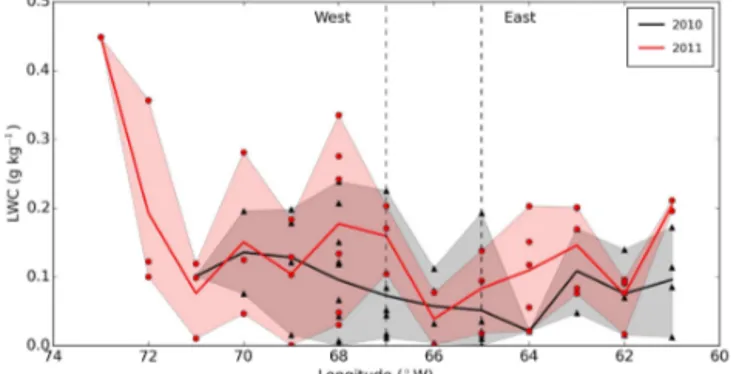
Figure 7.Same as Fig. 4 but for the liquid water content (LWC, g kg−1).
Figure 8.Same as Fig. 4 but for the number concentration of ice crystals (L−1).
1997; Chubb et al., 2016). Table 2 gives the statistical sig-nificance of differences between both sides of the peninsula as well as differences between both years, using at test. The most significant difference (at the 99 % level) for liquid drops is in the east of the peninsula between 2010 and 2011. A less significant but still noticeable difference exists between ei-ther side of the peninsula in 2011 (90 %). These relationships were not found in 2010 (< 80 %).
The LWC in clouds averaged by longitude for the 2 years is shown in Fig. 7. Again to get better statistics, the values of LWC have been averaged on both sides of the peninsula using the same size longitude bins that were used for liquid drop numbers. A significant difference between the 2 years is found at the 90 % level in the east and 95 % level in the west (see Table 2), although the east–west difference in both years is not significant. The single point of high LWC in 2011 at 73◦
W is the result of a small number of flights into active frontal systems with large amounts of liquid water.
3.2 Ice phase in clouds
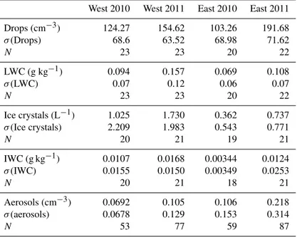
Table 1.Average values for cloud measurements and out-of-cloud aerosols for both years and both sides of the peninsula.σ(x) refers to the standard deviation of the variablex, andNthe number of flight averages available for the global eastern or western averages. LWC refers to liquid water content, and IWC to ice water content.
West 2010 West 2011 East 2010 East 2011
Drops (cm−3) 124.27 154.62 103.26 191.68 σ(Drops) 68.6 63.52 68.98 71.62
N 23 23 20 22
LWC (g kg−1) 0.094 0.157 0.069 0.108 σ(LWC) 0.07 0.12 0.06 0.07
N 23 23 20 22
Ice crystals (L−1) 1.025 1.730 0.362 0.737 σ(Ice crystals) 2.209 1.983 0.543 0.771
N 20 21 19 21
IWC (g kg−1) 0.0107 0.0168 0.00344 0.0124 σ(IWC) 0.0155 0.0150 0.00349 0.0253
N 20 21 18 21
Aerosols (cm−3) 0.0692 0.105 0.106 0.218 σ(aerosols) 0.0678 0.129 0.153 0.314
N 53 77 59 87
Table 2.Statistical significance of the differences between either year on either side of the peninsula as obtained from thettest performed for the four cloud variables and the aerosols (see text for details). Values greater than 90 % are highlighted in bold.
N(drops) LWC N(ice) IWC N(aerosols)
W2010–W2011 83 % 96 % 71 % 79 % 93 % E2010–E2011 99 % 94 % 91 % 85 % 98 % E2010–W2010 68 % 78 % 77 % 94 % 88 % E2011–W2011 93 % 89 % 96 % 50 % 99 %
Figure 9.Same as Fig. 4, for the ice water content (IWC, g kg−1).
number of ice particles observed is roughly 5 to 6 orders of magnitude lower than the number of cloud droplets, and the relative amplitude of the variability higher (the standard de-viation of liquid droplet number concentration is about 50 % of the average values, while it is as high as or higher than averages for ice crystal number concentrations). Also, not all the clouds investigated were glaciated to any extent, and
so there are slightly fewer measurements (Table 1) for ice crystals than for the drops – except for the east of the penin-sula in 2010 when there was an observation of a completely glaciated cloud. First looking at the number concentration of crystals, Fig. 8 and Table 1 show that in 2011 there were more crystals on both sides of the peninsula than in 2010. However, Table 1 shows the standard deviation of the crystal numbers is large. Table 2 shows that differences are not significant be-tween the 2 years (< 80 %) in the west, but significant in the east (90 %). Differences are also significant between either side of the peninsula in 2011 (at the 95 % level), however not in 2010 (77 %).
The ice water content (Fig. 9) shows a similar trend to crystal numbers in Fig. 8. However, in this case using the averaged values on each side of the peninsula (Table 1), the difference between both sides in 2010 is significant at the 90 %level.
The distribution of crystals with atmospheric temperature for the 2 years is shown in Fig. 10. Median ice crystal number concentrations have been derived over 0.5◦C bins along with
Figure 10.Distribution of ice crystals (L−1) as a function of atmo-spheric temperatures for 2010 (top row) and 2011 (bottom row), for the western side (left column) and for eastern side (right column). The median of the number concentrations was derived per 0.5◦C
bins. The dotted and dashed lines show the predicted number of pri-mary ice particles from two parameterization schemes (see text for details). The shaded area represents the median absolute deviation from the median value. West refers to 74–67◦W, and east refers to
65–60◦W.
are very different in the 2 years and between the east and west of the peninsula. In the west, both years have a peak ice num-ber concentrations around−5◦C. As reported by Grosvenor
et al. (2012), for some of the 2010 flights only, this peak is most probably related to a secondary ice production process known as the Hallett–Mossop process (Hallett and Mossop, 1974). This consists of droplets shattering upon freezing when impinged by existing crystals (riming process), thus causing a cascade of crystals. This process only operates ef-ficiently in a narrow temperature range (approximately−3 to
−8◦
C) with an optimum around−5◦
C and requires a large enough ratio of number concentrations of small drops (nS; < about 13 µm) to large drops (nL; > about 24 µm) (Mossop, 1985). Typical observed concentrations by Mossop (1985) of large (small) drops were 10–80 cm−3(5–60 cm−3), with the ratio nS/nL ranging between 0.1 and 5. In the present work, median values per flight for nS, nL, and nS/nL (where peaked concentrations are observed at−5◦C) are in the
fol-lowing respective ranges: 16–90 cm−3, 9–33 cm−3, and 0.5– 13 (with flight minima always above 0.1). Note that no con-strain is available in the present dataset to properly estimate the velocity of the riming particles. However, Mossop (1985) suggests that splintering can occur at velocities as low as 0.2 m s−1 and observes no abrupt drop of splinter
produc-tion from 1 to 0.55 m s−1, meaning that the rimer veloc-ity does not show a lower cut-off preventing the Hallett– Mossop process from happening. In addition, other mech-anisms known to trigger ice multiplication do not operate in the−8 to−3◦C temperature range but at colder temperatures
(<−10◦C), for example ice–ice collision (Takahashi et al.,
1995 and Yano and Phillips, 2011); freezing of large drops with ice spicules formation (Lawson et al., 2015); or breakup of crystals, which preferably requires irregular shapes like dendrites that are favoured at low temperatures (Bacon et al., 1998). The main limitation to an absolute identification of the process as Hallett–Mossop is the resolution (both tempo-ral and spatial) of the CAPS probe to observe the process in detail from its start as only the resulting larger crystals are observed and not the first ice.
In the east there is no clear peak at the high temperatures (>−10◦C) in 2011; there is only a small peak in 2010. It
sug-gests that relatively less secondary ice production is observed for the eastern side of the peninsula. It can be seen that dur-ing 2011 the number of ice crystals increases from−10◦C
to around−20◦C, and this probably corresponds to primary
ice production (where an INP active at a given temperature interacts with a droplet or vapour to form one crystal). Ice nu-clei parameterizations relying either only on the temperature (Cooper, 1986) or on both the temperature and the aerosol (> 0.5 µm) concentration (DeMott et al., 2010) are plotted in Fig. 10. They are meant to account for primary ice nucle-ation and predict increasing INP concentrnucle-ations from−10 to−20◦
C. For the DeMott et al. (2010) parameterization, aerosol concentrations bracketing the present average obser-vations (Sect. 3.3, Fig. 11) were used as input. Comparing the trends of either of the parameterizations to the ice crystal distributions also strengthens the idea that the ice crystal dis-tributions peaking around−5◦C are related to secondary ice
production processes.
3.3 Aerosols out of clouds
Figure 11. Same as Fig. 4 but for the number concentration of aerosols larger than 0.5 µm and smaller than 1 µm in diameter (cm−3). Fifty-five flights are considered here (31 flights from both campaigns equipped with the CAPS probe but not intended for cloud measurements in addition to the 24 cloud flights) to increase the statistics and give better overview of the aerosol population across the peninsula for both years. See text (Sect. 3.3) for more details. The vertical dashed lines delimit the western and eastern regions of the peninsula as defined in this study.
and is considered an anomaly), the 2 years to the west of the peninsula are very similar. To the east there is a sig-nificant difference between the 2 years (at the 95 % level), with 2011 having almost twice the concentration of aerosol as 2010. In 2011 there is also a significant difference between the east and west sides of the peninsula (at the 99 % level), with twice the concentration of aerosol in the east as in the west of the peninsula. Importantly, the same conclusions are drawn when using the 24 cloud flights only.
4 Discussion
The variability of cloud droplets and ice concentration ob-served in this study is quite large, and the number of flights is small, compared to the number of measurements that have been made at mid-latitudes. This makes identifying statisti-cally significant changes between geographical areas or be-tween years difficult. This problem has been dealt with by first averaging the data into longitudinal bands (Figs. 6–9 and 11). Although this allows some of the differences of interest to be observed, there are still too few points to determine if these differences are significant. To help with this, averages were taken of all the data on each side of the peninsula (Ta-ble 1), and in this case clear statistical differences can be seen (Table 2).
4.1 Aerosol source regions and liquid droplets
The average number of cloud droplets in the clouds (see Fig. 6) varies over a large range from just a few to almost 300 cm−3, and this probably reflects the large range in CCN found in the coastal areas of Antarctica. The mean droplet number concentration on each side of the peninsula is not untypical of values found in the mid-ocean (Pruppacher and
Figure 12.Location and altitudes (colour-coded, in m) of low-altitude (≤300 m above ground) air masses 48 h prior to reaching a flight track (from either of the 55 flights used in Fig. 11) west (left column) or east (right column) of the peninsula. Over-plotted is the monthly averaged sea ice fractional coverage as obtained from Nimbus-7 SMMR daily data at 25 km resolution (see text for refer-ence) (lightest blue is>90 %, darkest blue is 50 %, dark magenta is 25 %, and lightest magenta is below 1 %). West refers to 74–67◦W,
and east refers to 65–60◦W.
Klett, 1997; Chubb et al., 2016) and reflects the position of Rothera exposed to air masses with origins in the South Pa-cific. Table 2 shows that it is only in the east that there is a significant difference (at the 99 % level) between the 2 years in the aerosol concentration, and this might be a result of the different source regions for particles between the 2 years.
Table 3.Relative proportion of low-altitude (< 300 m) air masses passing over sea-ice-covered regions with respect to the total num-ber of low-altitude air masses along all back trajectories derived from the HYSPLIT model for 55 flight tracks from both campaigns (see text for details). In parentheses, the same percentages but for the 24 flights only. Relative proportions are indicated for both years and both sides of the peninsula, with the side referring to the (start) ending point of the air mass (back) trajectory. Percentages are com-puted over different time ranges, prior to reaching a given point of a flight track on either side. A region is considered as covered by sea ice as long as the sea ice concentration from the NIMBUS-7 SMMR is larger than 1 % (see Sect. 4.1 for reference).
East 2011 East 2010 West 2011 West 2010
Last 72 h 61 % (43) 35 % (47) 37 % (21) 24 % (9) Last 48 h 58 % (80) 45 % (60) 37 % (22) 25 % (8) Last 24 h 48 % (94) 68 % (91) 34 % (26) 26 % (8) Last 12 h 97 % (100) 90 % (98) 33 % (19) 15 % (7)
Figure 13. Averaged vertical profiles of number concentration of aerosols (cm−3) on both sides of the peninsula over all the flights (as for Fig. 11). Shaded areas indicate the spread of the data between absolute minimum and maximum values at each level. West refers to 74–67◦W, and east refers to 65–60◦W.
appears between 2010 and 2011, with 2011 showing more sources above the sea ice. Table 3 summarizes the relative proportion of air masses passing above sea ice compared to above open water/ice shelf (referred to as “other”) among all low-altitude air masses (i.e. below 300 m, approximate boundary layer height; Fiedler et al., 2010) and along all the back trajectories. The relative proportions are also indicated for the case when only the 24 cloud flights are used (number in parentheses in Table 3). We first comment on the anal-ysis using the 55 flights. A sea-ice-covered region was de-fined as a region where fractional coverage is larger than 1 % (however the sea ice regions of interest in Table 3 normally
have much larger values; see Fig. 12). These low-altitude air masses will have greater sensitivity to surface aerosol emis-sions. The statistics integrated over different durations are shown to illustrate the consistently dominating or increasing trends of the relative contributions of sea-ice low-altitude air masses among all low-altitude air masses. Whatever the time interval, low-altitude air masses sampled to the east of the peninsula always overpass sea ice regions relatively more of-ten than they overpass other regions – with the influence of the sea ice being greater in 2011. Looking at Table 3, we can see that the sea ice has most influence, over most time pe-riods, in the east in 2011, then less in the east in 2010, less again in the west in 2011, and least in the west in 2010. Thus, Table 3, along with Fig. 12, shows that (a) air sampled in the east is more sea-ice-influenced than air sampled in the west in both years, (b) air sampled in the east in 2011 has had a rel-atively longer sea ice track at low altitudes than in 2010, and (c) air sampled in the west in 2011 is more sea-ice-influenced than in 2010. Looking at the analysis restrained over the 24 cloud flights only, the above (b) statement becomes less clear as only the analysis over the period covering the previous 48 h shows a clear increase of sea ice influence in the east in 2011 (Table 3, second line), compared to 2010, but statement (a) and (c) still prevail and are even strengthened when con-sidering these smaller statistics. Overall clear differences ap-pear in the origin of the air masses when splitting the analysis into west–east and 2010–2011 comparisons. The larger con-centration of aerosols in 2011, especially on the eastern side (Fig. 11), compared to 2010 (Table 2) could be explained by more air masses having longer tracks at low level over sea-ice-covered regions of the Weddell Sea. It is possible that sea salt on the snow-covered surface of the sea ice could easily be lofted into the air as blowing snow which sublimes to form sea salt aerosol. This has been suggested as an efficient mech-anism for getting sea salt aerosol, which could act as CCN, into the boundary layer (Yang et al., 2008). This suggests that the increase in droplet number concentrations seen in 2011 on the eastern side of the peninsula (Fig. 6) could result from the increase in aerosol numbers. Figure 13 shows aver-age vertical profiles of aerosol number concentration on both sides of the peninsula for 2010 (blue circle) and 2011 (red tri-angles), for the 55 flights used in Sect. 3.3 (note that the same vertical profiles plotted with the 24 cloud flights show similar differences between the years). The corresponding shaded ar-eas indicate absolute minimum and maximum (non-null) val-ues at each altitude level over the respective campaigns. Like the latitudinal averages of aerosols shown in Fig. 11, Fig. 13 shows that the interannual differences in aerosol concentra-tion on the eastern side are much more pronounced (see the 99 % significance level in Table 2) than on the western side (93 % significance level). Interestingly, these differences oc-cur almost exclusively below 2000–2500 m. Above that al-titude, the concentration of aerosols is similar between both years and both sides (around 0.1–0.2 cm−3). The central part of the peninsula between 67◦
W and 65◦
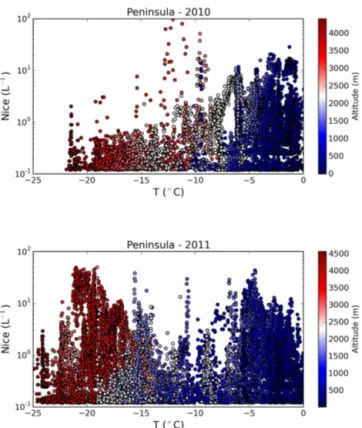
character-Figure 14.Distribution of all measurements of ice crystals (g−1) as a function of atmospheric temperatures for 2010 (top) and 2011 (bottom) for the whole peninsula. Colour indicates the altitude of the measurement, with light to dark red referring to increasing alti-tudes above≈2500 m and colours from light to dark blue referring to altitudes decreasing below≈2250 m.
ized by this concentration of about 0.1 cm−3 (not shown). This suggests that a homogeneous mixture of aerosols (at least in terms of number concentration, if not nature) pre-vails at altitudes above the height of the peninsula mountain barrier. Conversely, at lower levels, the Antarctic Peninsula barrier would help sustain different pools of aerosols on ei-ther of its sides. These aerosol pools could give rise to differ-ent cloud microphysics on either side of the peninsula, and a possible interpretation of the observations is that the in-creased number of droplets in the east in 2011 compared to 2010 could be the result of an environment more influenced by particle originating from sea ice regions.
4.2 Ice production, altitude ranges, and aerosols Interestingly, the ice crystal number concentration (Fig. 8) does not follow the same pattern as the liquid droplets. A significant difference (at the 95 % level) is seen between the 2 years in the west, and a similar significant difference is also seen between both sides of the peninsula in 2011. How-ever, this is not unexpected as, while aerosols are the source of CCN and INPs so that a correlation between the numbers of liquid drops and ice crystals might be expected, there is
another process going on to create ice crystals. This is the secondary ice production due to the Hallett–Mossop pro-cess for temperatures warmer than −10◦C (introduced in
Sect. 3.2). The peak of ice crystal numbers at temperatures above −10◦C can be clearly seen (Fig. 10), especially in
the west, where as might be expected the temperatures are warmer. This is illustrated by Fig. 4, which shows each year’s temperatures averaged by latitude along the aircraft tracks. In the east there is much less evidence of secondary ice forma-tion for both years (Fig. 10), and this correlates with the sim-ilarly lower temperatures in both years (Fig. 4). At tempera-tures below−10◦
C (Fig. 10) it can be seen that in 2011 there is a distinct peak in ice concentration, which suggests more primary ice production (see Sect. 3.2) in both the west and the east at temperatures approximately ranging between−10
and−20◦C, while there is almost virtually no primary ice
production peak in 2010. Figure 14 shows the entire dataset of crystal distribution with temperatures for the 2 years (both sides at the same time) colour-coded with the altitude of the observation. The primary ice production mainly occurs at al-titudes above roughly 2500 m, while the secondary ice pro-duction occurs almost exclusively below 2000 m – this of course is related to atmospheric lapse rate. This means that the primary ice production peak presence cannot be solely related to the increase of aerosols, which is observed mostly below 2500 m (see Sect. 4.1). As such, the lower primary ice production in 2010, and its presence in 2011 on both sides of the peninsula, can be linked to the colder 2011 tempera-tures compared to the 2010 temperature above 2500 m (not shown). Another possible factor in the lower ice production in 2010 is the different nature of INPs due to different air mass histories. It can be seen that in 2011 more air masses were coming from above sea ice regions (see Sect. 4.1). It has been suggested that biogenic particles found in sea ice could act as INPs (Burrows et al., 2013), and the same method for transferring from sea ice to the atmosphere (as the sea salt) could explain the different nature of INPs found in 2011 above 2500 m, leading to more primary ice production in 2011.
5 Summary and conclusion
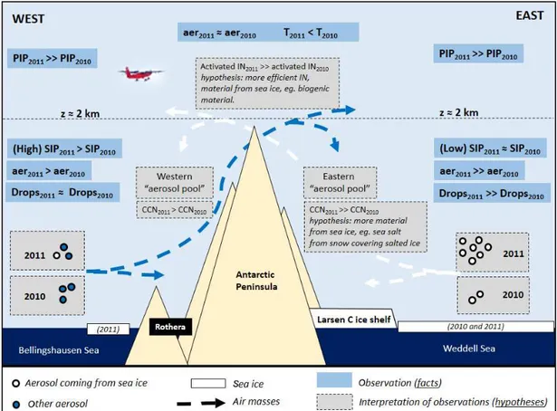
Figure 15 summarizes the results reported in this paper. Our observations show the significant differences in cloud prop-erties between the two measurement periods, February 2010 and January 2011, and between measurements made to the east and to the west of the Antarctic Peninsula, and they present some possible explanation for those.
Figure 15.Schematic summarizing main observations from aircraft measurements from both periods of interests (February 2010 and January 2011) and on both sides of the Antarctic Peninsula (blue rectangles), as well as hypotheses (grey-framed rectangles) proposed to explain observations, as presented in the Discussion (Sect. 4). PIP refers to primary ice production, while SIP refers to secondary ice production, as presented in Sect. 3.2.
2011, relatively more air masses were coming from the sea ice, and relatively more on the eastern side than on the west-ern side. This brings a possibly interesting explanation to the twice-larger number of droplets in 2011 in the east (approx-imately 200 cm−3)compared to 2010 in the east, and also 50 % larger than 2011 in the west.
The Hallett–Mossop secondary ice multiplication (at tem-peratures warmer than−10◦C, peaking around−5◦C)
pro-cess seems to be key to the ice production mechanism be-low 2500 m on both sides of the peninsula, and mainly on the warmer western side. In contrast above 2500 m the pri-mary ice production mechanism is expected to dominate. The larger production of primary ice crystals (at tempera-tures colder than −10◦
C, peaking around −20◦
C) above 2500 m in 2011 compared to 2010 on both sides of the penin-sula is due to colder temperatures (activating more INPs) and the possibly different nature of INPs (coming relatively more from above sea ice regions). Indeed, there is only a small increase in number concentration of large (> 0.5 µm) aerosols in 2011 above 2500 m. This is why the increase in aerosol number supports the larger amounts of liquid droplets but does not seemingly support the larger number of pri-mary ice seen above 2500 m in 2011 on both sides of the
peninsula. These observations show that the concentration of large aerosols (> 0.5 µm) is fairly similar across the peninsula (about 0.1–0.2 cm−3) at altitudes higher than the mountain barrier where dynamics would sustain a well-mixed aerosol population. Conversely, the mountains would favour the cre-ation of so-called aerosol pools on either side of the penin-sula, with different concentrations and nature that would be responsible for a different microphysics. Similarly, ice pro-duction is affected by the temperatures prevailing on ei-ther side of the peninsula, with little secondary ice produc-tion occurring on the eastern (colder) side and more on the (warmer) western side. The mountain’s height controls the altitude at which both sides display similar primary ice pro-duction peaks above 2500 m, because of similar population of aerosols.
global climate models (Flato et al., 2013; Bodas-Salcedo et al., 2014). Given that, in winter, sea ice can extend up to 60◦S and even 55◦S in some regions, sources of CCN and
INPs related to the sea ice could potentially have a large im-pact on the microphysics of clouds forming over the Southern Ocean, as they seem to have across the Antarctic Peninsula.
The present study is the very first of its kind attempting to depict cloud microphysics and aerosols across the Antarc-tic Peninsula from a small amount of flights; the scenario we suggest hopefully will stimulate other studies and measure-ments to better assess the plausibility of our interpretations.
6 Data availability
The data are being formatted for inclusion in the Polar Data Centre and will be available soon.
Acknowledgements. This work would not have been possible without the help of the scientists and support staff who helped in the Antarctic. We thank the editor and two anonymous reviewers for their comments, which helped improve the manuscript. The work was funded by UK Natural Environment Research Council with core funding and under grant NE/K01305X/1 and under NERC grant NEB1134.
Edited by: M. Krämer
Reviewed by: two anonymous referees
References
Bacon, N. J., Swanson, B. D., Baker, M. B., and Davis, E. J.: Breakup of levitated frost particles, J. Geophys. Res., 103, 13763–13775, 1998.
Baumgardner, D., Jonsson, H., Dawson, W., O’Connor, D., and Newton, R.: The cloud, aerosol and precipitation spectrometer: a new instrument for cloud investigations, Atmos. Res., 59–60, 251–264, doi:10.1016/S0169-8095(01)00119-3, 2001.
Belosi, F., Santachiara, G., and Prodi, F.: Ice-forming nuclei in Antarctica: New and past measurements, Atmos. Res., 145–146, 105–111, doi:10.1016/j.atmosres.2014.03.030, 2014.
Bodas-Salcedo, A., Williams, K. D., Ringer, M. A., Beau, I., Cole, J. N. S., Dufresne, J.-L., Koshiro, T., Stevens, B., Wang, Z., and Yokohata, T.: Origins of the Solar Radiation Biases over the Southern Ocean in CFMIP2 Models*, J. Climate, 27, 41–56, doi:10.1175/JCLI-D-13-00169.1, 2014.
Bromwich, D. H., Nicolas, J. P., Hines, K. M., Kay, J. E., Key, E. L., Lazzara, M. A., Lubin, D., McFarquhar, G. M., Gorodetskaya, I. V., Grosvenor, D. P., Lachlan-Cope, T., and Van Lipzig, N. P. M.: Tropospheric clouds in Antarctica, Rev. Geophys., 50, 1–40, doi:10.1029/2011RG000363, 2012.
Bromwich, D. H., Otieno, F. O., Hines, K. M., Manning, K. W., and Shilo, E.: Comprehensive evaluation of polar weather research and forecasting model performance in the Antarctic, J. Geophys. Res.-Atmos., 118, 274–292, doi:10.1029/2012JD018139, 2013.
Brown, P. R. A. and Francis, P. N.: Improved Measurements of the Ice Water Content in Cirrus Using a Total-Water Probe, J. Atmos. Ocean. Tech., 12, 410–414, doi:10.1175/1520-0426(1995)012<0410:IMOTIW>2.0.CO;2, 1995.
Burrows, S. M., Hoose, C., Pöschl, U., and Lawrence, M. G.: Ice nuclei in marine air: biogenic particles or dust?, Atmos. Chem. Phys., 13, 245–267, doi:10.5194/acp-13-245-2013, 2013. Cavalieri, D. J., Parkinson, C. L., Gloersen, P., and Zwally, H.
J.: Sea Ice Concentrations from Nimbus-7 SMMR and DMSP SSM/I-SSMIS Passive Microwave Data, Version 1, Sea Ice Con-centrations from Nimbus-7 SMMR, Boulder, CO, USA, NASA National Snow and Ice Data Center Distributed Active Archive Center, available at: doi:10.5067/8GQ8LZQVL0VL (last access: January 2016), 1996.
Chubb, T., Huang, Y., Jensen, J., Campos, T., Siems, S., and Man-ton, M.: Observations of high droplet number concentrations in Southern Ocean boundary layer clouds, Atmos. Chem. Phys., 16, 971–987, doi:10.5194/acp-16-971-2016, 2016.
Cooper, W. A.: Ice Initiation in Natural Clouds, Meteor. Mon., 21, 29–32, doi:10.1175/0065-9401-21.43.29, 1986.
Crosier, J., Bower, K. N., Choularton, T. W., Westbrook, C. D., Con-nolly, P. J., Cui, Z. Q., Crawford, I. P., Capes, G. L., Coe, H., Dorsey, J. R., Williams, P. I., Illingworth, A. J., Gallagher, M. W., and Blyth, A. M.: Observations of ice multiplication in a weakly convective cell embedded in supercooled mid-level stratus, At-mos. Chem. Phys., 11, 257–273, doi:10.5194/acp-11-257-2011, 2011.
DeMott, P. J., Prenni, A. J., Liu, X., Kreidenweis, S. M., Petters, M. D., Twohy, C. H., Richardson, M. S., Eidhammer, T., and Rogers, D. C.: Predicting global atmospheric ice nuclei distributions and their impacts on climate, P. Natl. Acad. Sci. USA, 107, 11217– 11222, doi:10.1073/pnas.0910818107, 2010.
Elvidge, A. D., Renfrew, I. A., King, J. C., Orr, A., and Lachlan-Cope, T. A.: Foehn warming distributions in nonlinear and linear flow regimes: a focus on the Antarctic Peninsula, Q. J. Roy. Me-teor. Soc., 142, 618–631, doi:10.1002/qj.2489, 2014.
Fiedler, E. K., Lachlan-Cope, T. A., Renfrew, I. A., and King, J. C.: Convective heat transfer over thin ice covered coastal polynyas, J. Geophys. Res., 115, C10051, doi:10.1029/2009JC005797, 2010. Flato, G., Marotzke, J., Abiodun, B., Braconnot, P., Chou, S. C., Collins, W., Cox, P., Driouech, F., Emori, S., Eyring, V., For-est, C., Gleckler, P., Guilyardi, E., Jakob, C., Kattsov, V., Rea-son, C., and Rummukainen, M.: Evaluation of Climate Mod-els, Clim. Chang. 2013 Phys. Sci. Basis. Contrib. Work. Gr. I to Fifth Assess. Rep. Intergov. Panel Clim. Chang., 741–866, doi:10.1017/CBO9781107415324, 2013.
Bedmap2: improved ice bed, surface and thickness datasets for Antarctica, The Cryosphere, 7, 375–393, doi:10.5194/tc-7-375-2013, 2013.
Grosvenor, D. P., Choularton, T. W., Lachlan-Cope, T., Gallagher, M. W., Crosier, J., Bower, K. N., Ladkin, R. S., and Dorsey, J. R.: In-situ aircraft observations of ice concentrations within clouds over the Antarctic Peninsula and Larsen Ice Shelf, Atmos. Chem. Phys., 12, 11275–11294, doi:10.5194/acp-12-11275-2012, 2012. Hallett, J. and Mossop, S. C. C.: Production of secondary ice particles during the riming process, Nature, 249, 26–28, doi:10.1038/249026a0, 1974.
King, J. C., Lachlan-Cope, T. A., Ladkin, R. S., and Weiss, A.: Airborne Measurements in the Stable Boundary Layer over the Larsen Ice Shelf, Antarctica, Bound.-Lay. Meteorol., 127, 413– 428, doi:10.1007/s10546-008-9271-4, 2008.
King, J. C., Gadian, A., Kirchgaessner, A., Kuipers Munneke, P., Lachlan-Cope, T. A., Orr, A., Reijmer, C., van den Broeke, M., van Wessem, J., and Weeks, M.: Validation of the summertime surface energy budget of Larsen C Ice Shelf (Antarctica) as rep-resented in three high-resolution atmospheric models, J. Geo-phys. Res., 1335–1347, doi:10.1002/2014JD022994, 2015. Lachlan-Cope, T.: Antarctic clouds, Polar Res., 29, 150–158,
doi:10.1111/j.1751-8369.2010.00148.x, 2010.
Lachlan-Cope, T. A., Ladkin, R., Turner, J., and Davison, P.: Obser-vations of cloud and precipitation particles on the Avery Plateau, Antarctic Peninsula, Antarct. Sci. 13, 339–348, 2001.
Lawson, R. P., Woods, S., and Morrison, H.: The Microphysics of Ice and Precipitation Development in Tropical Cumulus Clouds, J. Atmos. Sci., 72, 2429–2445, doi:10.1175/JAS-D-14-0274.1, 2015.
Mossop, S. C.: Secondary ice particle production during rime growth: the effect of drop size distribution and rimer velocity, Q. J. Roy. Meteol. Soc., 111, 1113–1124, 1985.
Pruppacher, H. R. and Klett, J. D.: Microphysics of Clouds and Pre-cipitation, Kluwer Academic Publishers, Dordrecht, the Nether-lands, 1997.
Saxena, V. K.: Evidence of the Biogenic Nuclei Involvement in Antarctic Coastal Clouds, J. Phys. Chem., 87, 4130–4134, 1983. Stein, A. F., Draxler, R. R., Rolph, G. D., Stunder, B. J. B., Cohen, M. D., and Ngan, F.: NOAA’s HYSPLIT atmospheric transport and dispersion modeling system, B. Am. Meteorol. Soc., 2015, 2059–2077, doi:10.1175/BAMS-D-14-00110.1, 2015.
Takahashi, T., Nagao, Y., and Kushiyama, Y.: Possible High Ice Particle Production during Graupel–Graupel Collisions, J. Atmos. Sci., 52(24), 4523–4527, doi:10.1175/1520-0469(1995)052<4523:PHIPPD>2.0.CO;2, 1995.
Taylor, J. W., Choularton, T. W., Blyth, A. M., Liu, Z., Bower, K. N., Crosier, J., Gallagher, M. W., Williams, P. I., Dorsey, J. R., Flynn, M. J., Bennett, L. J., Huang, Y., French, J., Korolev, A., and Brown, P. R. A.: Observations of cloud microphysics and ice formation during COPE, Atmos. Chem. Phys., 16, 799–826, doi:10.5194/acp-16-799-2016, 2016.
Thompson, G. and Eidhammer, T.: A study of aerosol impacts on clouds and precipitation development in a large winter cyclone, J. Atmos. Sci., 71, 3636–3658, doi:10.1175/JAS-D-13-0305.1, 2014.
Yang, X., Pyle, J. A., and Cox, R. A.: Sea salt aerosol production and bromine release: Role of snow on sea ice, Geophys. Res. Lett., 35, L16815, doi:10.1029/2008GL034536, 2008.