Precificação da opção de recompra nas operações de venda descoberta: abordagem empírica...

(1)

Universidade de São Paulo

Faculdade de Economia, Administração e Contabilidade

Departamento de Economia

Programa de Pós-Graduação em Economia

Short Selling Recall Option Pricing:

empirical and theoretical approaches

Precificação da Opção de Recompra em Operações de Venda Descoberta:

abordagens empírica e teórica

Leonardo Viana de Almeida

Dissertação apresentada ao Programa de Pós-Graduação em Economia do Departamento de Economia da Faculdade de Economia, Administração e Contabilidade da Universidade de São Paulo, como requisito parcial para a obtenção do título de Mestre em Ciências.

Orientador: Prof. Dr. Fernando Daniel Chague

Versão Corrigida

(versão original disponível na Faculdade de Economia, Administração e Contabilidade)

São Paulo

(2)

Universidade de São Paulo

Faculdade de Economia, Administração e Contabilidade

Departamento de Economia

Programa de Pós-Graduação em Economia

Short Selling Recall Option Pricing:

empirical and theoretical approaches

Precificação da Opção de Recompra em Operações de Venda Descoberta:

abordagens empírica e teórica

Leonardo Viana de Almeida

Dissertação apresentada ao Programa de Pós-Graduação em Economia do Departamento de Economia da Faculdade de Economia, Administração e Contabilidade da Universidade de São Paulo, como requisito parcial para a obtenção do título de Mestre em Ciências.

Orientador: Prof. Dr. Fernando Daniel Chague

Versão Corrigida

(versão original disponível na Faculdade de Economia, Administração e Contabilidade)

São Paulo

(3)

(4)

Prof. Dr. Marco Antonio Zago Reitor da Universidade de São Paulo

Prof. Dr. Adalberto Américo Fischmann

Diretor da Faculdade de Economia, Administração e Contabilidade

Prof. Dr. Hélio Nogueira da Cruz Chefe do Departamento de Economia

Prof. Dr. Márcio Issao Nakane

(5)

Dedicatória e Agradecimentos:

• Agradeço meu Orientador, Prof. Dr. Fernando Daniel Chague, pela força desprendida nesta empreitada.

• Agradeço meus pais, Ana Luiza d’Ávila Viana e Márcio Wohlers de Almeida por me acompanharem ao longo deste grande desafio.

• Dedico este trabalho aos meus avôs, Prof. Dr. Valdemar Ferreira de Almeida e

(6)

ABSTRACT

Short selling is important for price efficiency as it helps negative information to be incorporated into prices. As short selling requires borrowing stock in advance, the equity lending market plays a central role in price efficiency. For instance, when the costs of borrowing certain equities are high, these stocks are likely to be overpriced. Unfortunately, not much is known about the equity lending market, particularly the Brazilian market. Here, we have investigated a particular feature of the equity lending contract, namely, the lender recall option. Lending contracts either i) allow the lender to recall the stock at an earlier date than initially agreed, or ii) allow no early recall, that is, they are fixed term contracts. We have derived a simple model for recall option pricing and confirmed the model empirically.

(7)

Precificação da Opção de Recompra em Operações de Venda Descoberta:

abordagens empírica e teórica

RESUMO

A venda descoberta desempenha uma importante participação na eficiência da precificação de ativos, pois permite incorporar informações negativas aos seus preços. Como a venda descoberta requer que um ativo seja alugado previamente, o mercado de aluguel de ativos tem um papel central na formação eficiente de preços. Por exemplo, quando os custos de aluguel são altos, ativos estão provavelmente sobrevalorizados. Infelizmente pouco se conhece a fundo sobre o mercado de aluguel de ativos. Neste artigo, investigamos uma característica do aluguel de ações, propriamente dita, a opção de liquidação antecipada pelo doador. Contratos de aluguel, quanto a este aspecto, podem i) permitir que o doador requeira suas ações antes do prazo acordado ou ii) não permitir esta opção, possuindo prazo fixo. Derivamos um modelo simples de precificação desta opção e confirmamos o modelo empiricamente.

(8)

List of Figures

Figure 1: Monthly proportion of recall option...………..…..…….….. 10

Figure 2: Borrower’s preference value: recall probability variation

among several loan fee drifts………...………..………..……... 17

Figure 3: Borrower’s preference value: recall frequency variation,

fixed loan fee drift, different loan fee shares ………...……...…….….. 18

Figure 4: Borrower’s preference value: loan fee drift variation

among different recall probabilities……….……….…...……. 18

Figure 5: Borrower’s preference value: stochastic share variation,

fixed loan fee drift, different recall probabilities.…………...……...…….….. 19

Figure 6: Four-step binomial tree stock price process ………....…….…. 21

Figure 7: Lender preference value: expected return, risk-free rate variation

among several loan fees.……...………...……….… 24

Figure 8: Lender’s preference value: expected return, loan fee variation

among several risk-free interest rates..……….…... 24

Figure 9: Lender preference value: expected return, volatility variation…………..… 25

Figure 10: Lender preference value: multiple expected returns, risk-free

rate variation…….………..……….………….….... 25

Figure 11: Lender preference value: negative expected return, risk-free

rate variation…….……….. 26

Figure 12: Lender preference value: negative expected return, risk-free

(9)

List of Tables

Table 1: Brazilian loan market: Annual aggregate figures…………..…………..…….. 7

Table 2: Brazilian loan market: Participation in 2015 according to investor type……. 7

Table 3: Herfindahl-Hirschman index: Cross-sectional descriptive statistics

in terms of the 55 most liquid tickers ………...……..………. 32

in terms of the 100 most liquid tickers………...….…………. 32

in terms of the 150 most liquid tickers…….…………..………...………. 32

Table 6: Regression results for Equation 14 in terms of the 55 most liquid

stocks………….……….………..……….. 35

stocks……….………...………... 36

stocks………..…………..……….. 37

Table 9: Regression results for Equation 14 in terms of 150 most liquid

stocks…….………..….…….……….………..……....…. 37

stocks……….……….………….………..………..… 38

stocks……….…….……….………….…..……….… 38

Table 12: Regression results for Equation 16, in terms of the 55 most liquid

(10)

stocks…………..………..………… 39

stocks………..………..… 39

stocks………..………..……… 40

Table16: Regression results for Equation 17 in terms of the 100 most liquid

stocks………...………..…… 41

Table17: Regression results for Equation 17 in terms of 150 most liquid

stocks………..……..………..………….………….………… 41

Table 18: Main statistics for the 150 most liquid tickers: loan fee statistics

(11)

List of Symbols and Abbreviations

BM&F BOVESPA: Brazilian Securities, Commodities and Futures Exchange (Bolsa de Valores, Mercadorias e Futuros de São Paulo)

FE: Fixed Effect

HHI: Herfindahl-Hirschman Index

𝜇, 𝜎 : Normal distribution with mean 𝜇 and variance 𝜎

(12)

Summary

1. Introduction……….. 1

2. The loan market……….……..…….. 5

2.1 American and Brazilian loan markets………...……… 5

2.2 Loan market data: variables and features……….…………..……. 8

2.3 The Variable Recall option.……..………..……….……. 10

3. Theoretical model……….…… 12 3.1 Borrower’s Preference Value………..………....……. 13

3.2 Borrower’s Preference Value Simulation…...………..………..…… 17

3.3 Lender’s Preference Value…………..……….………..………. 20

3.4 Lender’s Preference Value Simulation………..…………..…..……… 23

3.5 Equilibrium model………..……….……..………...…. 28

4. Empirical analysis……….... 30

4.1 Initial results………..……….……. 30

4.2 Market concentration index……….……….… 31

4.3 Regression analysis……….. 33

5. Robustness……… 37

6. Concluding remarks……….……… 42

7. Bibliography………..……… 43

(13)

1

1. INTRODUCTION

Short selling is important for price efficiency as it helps negative information to be incorporated into prices. As short selling requires borrowing stock in advance, the equity lending market plays a central role in price efficiency. For instance, when the costs of borrowing certain equities are high, these stocks are likely to be overpriced. Unfortunately, not much is known about the equity lending market, particularly the Brazilian market. Here, we have investigated a particular feature of the equity lending contract, namely, the lender recall option. Lending contracts either i) allow the lender to recall the stock at an earlier date than initially agreed, or ii) allow no early recall, that is, they are fixed term contracts. We have derived a simple model for the recall option pricing and confirmed the model empirically.

From the lender’s perspective, the recall option is desirable as it allows the lender to sell the re-called stock at any time. As such, the lender would agree with a lower loan fee to have the recall option available. In turn, from the borrower’s perspective, the recall option is not desirable as an early recall by the lender means that the borrower will have to locate another owner willing to lend it or, as a last resource, buy it in the spot market. In this case, the borrower would also require a lower loan cost (fee) for recall option. Thus, from an economic perspective, loan contract with recall option available should have lower loan fees, that is, ceteris paribus.

In order to show that loan contracts with recall option actually present lower loan fees, we used a comprehensive data set containing all stock loan contracts closed in Brazil from January 2009 to July 2011. Interestingly, our panel regressions show that the recall option does involve lower loan fees, but only in some circumstances. For instance, the recall option is to be priced in deals closed only when the conditions of equity lending market are unfavorable to the borrowers. That is, the loan fee is lower for deals in which recall option is available only when borrowers are likely to have a hard time locating new lenders.

(14)

2 and brokers offering a large quantity of stock, the index approaches zero, whereas when there are fewer lenders and brokers the index approaches one. At the limit the index is set to one, corresponding to a case of monopoly. The market concentration index, in this case, is a measure of how hard it is for borrowers to find a particular stock available for loan, like a loan search cost proxy.

An interactive variable, combining the market concentration index with the lender recall option dummy, which assigns 1 to re-callable cases or zero otherwise, has been shown to be significant after being regressed by the loan fee as a dependent variable. The negative coefficient demonstrates that lenders accept a lower loan fee while borrowers demand a lower loan cost (fee) if loan is re-callable and market is scarce. We performed regressions by using different market concentration indexes for both lender and brokers as well as at monthly or weekly aggregated concentrations. Assuming that the market is highly concentrated, the recall option price varies from 0 to 3% a year.

To give some theoretical foundation for these empirical findings, we have proposed a theoretical pricing model which involves two different preference values before outputting the recall option price; one preference value obtained under the

borrower’s perspective and the other under the lender’s perspective (the latter being based on a particular rationale of an American option pricing model). The borrower’s preference value framework refers to his perspective and corroborates our empirical findings.

The borrower’s preference value approach is a flexible framework developed to accommodate the market concentration index, since it interferes with the impact of recall option on the loan fee. This framework establishes a loan fee process resulting in a new loan fee in the case of recall. The new fee changes in terms of both level and volatility, making use of market concentration as an argument. Through this new fee, the borrower can re-loan the stock after it is re-called, thus changing its final pay-off. The expected pay-off difference in such scenarios sets the preference value.

(15)

3 stock option. Both frameworks support our empirical results, as well as the variable impact dynamics.

A short sale position, simultaneously held with a long position, can be justified by a distinct expectation formed by investors regarding future returns. Short positions increase the spot market supply as its curve shifts towards right, hence lowering the asset prices. Therefore, short selling restrictions may lead to asset over-valuation (Miller, E.,1977).

The global financial crisis in 2007-2009 and its repercussions in the present day have frightened many market regulators around the world, who in response have restricted or even banned short selling positions. However, there are still major controversies among researchers about its impact on the market, which enhances the debate (Chague, F.; et al., 2014).

Duffie, Gârleanu & Pedersen (GDP model, 2002) proposed a model which includes the cost for finding assets available for renting (search cost) and therefore lenders may act as local monopolists, which results in positive loan fees, even in the presence of loan supply excess.

Kolansiski, Reed & Ringgenberg (KRR model, 2013) suggested proxies for search costs, such as firm’s size, bid-ask spread and stock concentration among lenders, and found that these variables raise both level and dispersion of loan fee as they intuitively increase search costs.

In 2015, Prado empirically tested the GDP model and observed that financial institutions increase their long positions as the loan fees of shares are raised, incorporating loan income into stock prices. As a final result, asset owners take into account loaning as a possible dividend gain, which raises the asset values (Prado, M., 2015).

(16)

4 opportunity for significant gain obtained by short selling 30-year new treasury bonds combined with buying (long position) 30 year-old bonds.

The evidence about the Brazilian equity lending market is incipient. Chague et al. (2015) have shown that the stock lending market is a market-based relationship, where low-cost borrowers (borrowers who face lower loan fees) are well connected to brokers who, in turn, are well connected to lenders who hold a large share of the lending market. The Brazilian stock loan market is highly inefficient. Our data show that some loan fees are three times higher than others for the same stock in similar quantities and on the same day.

In the American market, Avellaneda (2009) has proposed a model based on hard-to-borrow stocks (those which face regulatory short-selling restrictions or insufficient float available for lending): a dynamic model correlating stock price and buy-in rate (i.e. when the clearing chamber issues a buy order to the seller who has failed to deliver a previously sold stock). The author showed empirical evidence that buy-ins are followed by price jumps (Avellaneda, M., 2009).

(17)

5

2. THE LOAN MARKET

2.1 American and Brazilian Loan Markets

The Securities and Exchange Commission defines short sale as selling an asset (e.g. equity, private or public bonds) which does not currently belong to the seller or is not intended for delivery. Hence, in order to perform a short sale, the seller must rent it (D’Avolio, G., 2002).

One of the first large data collections from the American equity lending market was conducted by D’Avolio between April 2000 and September 2002, who combined data from several institutions and brokers intermediating loan contracts. The main empirical results are summarized bellow (D’Avolio, G., 2002):

• The aggregate loan market is quite liquid for lending any stock, whose average cost is 0.25% per year, and about 7% of the supply is in fact loaned.

• Most liquid stocks in the spot market are available for lending. Those unavailable for lending represent less than 1% of the market in value and are traded for very low nominal prices per share.

• Stocks of low nominal values with low liquidity are almost never loaned despite being available, representing 10% of the loan market in value.

• Institutional investors who lend abundant stocks usually offer large companies stocks with high liquidity, indicating that they are large passive funds that follow market indexes.

• 91% of the loans cost less than 1% per year, whereas the remaining 9% cost in average 4.3% per year.

• Some stocks are excessively expensive for lending; in general, they are of small companies with low cash-flow, high managerial turnover and poorly specified accounting books.

• Recall option is rarely taken; the monthly average is about 2% of the stocks loaned. The average time for recall option is 23 business days before contract expiry date. Within such events, the market volume may double and the short seller’s gains diminished, on average (D’Avolio, G., 2002).

(18)

6 database containing information such as offers available for loaning, volume, quantity, financial intermediates, deals closed, loan and brokerage fees, and investor type. This contrasts with most of the lending markets, which are decentralized with only partially available information.

Studies on these data are relatively recent, whereas empirical analyses of American data began decades ago.

The Brazilian equity loan market features a singular micro-structure, where all transactions are centralized through BM&F BOVESPA, the world’s fourth biggest stock exchange for equities, public and private bonds, future currency contracts, commodities, indexes and all sorts of derivatives.

The loan market is regulated by the Brazilian Securities and Exchange Commission and by the National Monetary Council.

Any asset traded by the stock exchange is available for loan, whose parties (i.e. lender and borrower) are intermediated by BM&F BOVESPA authorized brokers. The loan market has grown significantly in Brazil over the last decade. In 2011, transactions involved 290 companies per month involving individuals (40%), foreign investors (35%) and funds (25%) as lenders as well as funds (70%), foreign investors (25%) and individuals (5%) as borrowers (Chague, F.; et al., 2014).

As advertised by the Brazilian BM&F BOVESPA, equity or asset-rental activity increases the market liquidity, thus enhancing price efficiency and flexibility, which benefits investors with both short- and long-term strategies. A short sale trade requires the asset to borrowed, either in advance or after selling it on the spot market, by rewarding the lender with a loan fee freely settled between lender and borrower. The market requires mechanisms to balance the price settlement accordingly, with asset renting and short selling making a significant contribution.

Formally after lending the asset, the owner is no longer entitled to it and therefore does not receive any designated rights from the issuing company. The loan system is, however, in charge of reimbursing the lender on the same date with the same amount, just as it would be if the lender owned the asset. Similarly, the loan system also withdraws this amount from the borrower.

(19)

7

Table 1. Brazilian loan market’s annual aggregate figures

Year Volume (mi R$) Volume (mi US$) Number of Deals Number of Intermediates Number of Traded Assets

2006 109,674.05 50,496.18 271,210 1,002 1,869

2007 272,473.06 142,106.28 568,592 998 2,639

2008 303,505.51 174,568.50 627,414 1,000 3,006

2009 258,912.60 137,483.77 711,987 990 2,887

2010 465,605.78 265,892.32 971,558 999 3,125

2011 732,750.51 436,302.09 1,417,787 1,046 3,327

2012 785,927.87 405,854.85 1,313,355 1,019 3,322

2013 1,006,836.85 468,628.79 1,693,151 965 3,500

2014 735,017.70 321,967.85 1,518,369 935 3,481

2015 665,732.25 203,569.14 1,519,445 870 3,358

Source: BM&F BOVESPA (home/services/asset loan/variable income)

A significant market increase can be observed over the past decade until 2013, whether in volume, deals or traded assets, when the loan market roughly matched the spot market in volume (R$ 1.8 trillion). The reverse tendency occurred in the last two years due to the Brazilian economic recession in 2014 and 2015. The volume in US$ decreased even more severely due to the depreciation of the Brazilian currency.

Table 2. Brazilian loan market participation in 2015 according to investor type

Year Type Individuals Commercial Banks Social Retirement Funds Mutual Funds Other Civilian Social Associations Foreign Investors Private Enterprises

2015 Lender 15.59% 0.20% 1.59% 44.21% 1.09% 35.60% 1.71% Borrower 2.61% 2.37% 0.00% 48.25% 0.17% 45.83% 0.76% Source: BM&F BOVESPA (home/services/asset loan/variable income)

Table 2 shows that mutual funds are the main participant in the loan market, followed by foreign investors, both acting as lenders and borrowers, whereas individuals participate mostly as asset lenders.

The Brazilian market involves mainly over-the-counter transactions (90% of the deals), with only a few deals being made through electronic means, where offers are available.

(20)

8 found no evidence that such transactions manipulate the market or make prices unstable. Finally, there are indeed signs that privileged information benefits short seller agents (Chague, F.; et al. 2013 and 2014). Chague et al. have also shown that the use of electronic means by the loan market reduces both loan fee and volatility, thus encouraging its use in a market shadowed by the over-the-counter practice (Chague, et al., 2015, Brazilian equity lending market).

2.2 Loan Market Data: Variables and Features

The available data present all loan offers to both lenders and borrowers registered in Brazil from January 2009 to July 2011 on a daily basis (i.e. 3,359,354 offers). For every lender’s or borrower’s loan offer there is a unique offer code, including date, ticker code (i.e. firm’s share code), quantity (number of shares offered), loan fee, brokerage fee, lender’s, borrower’s and broker’s identification numbers (formed by a random number invariant over time which uniquely identifies investor or intermediate), offer status (closed, available, partially available, or canceled due to some specific reason), time length, investor type, lender recall option, and borrower return option. Lender recall option means that the lender is able, although not obliged, to request their shares prior to the loan expiration date. Borrower return option means that the borrower is able, although not obliged, to deliver their loaned shares prior to the loan expiration date.

In general, we can identify the following approximate participation according to investor type:

• Lenders: 41% of individuals, 33% of funds, 15% of foreign investors.

• Borrowers: 45% of funds, 30% of individuals, 16% of foreign investors.

As our dataset presents both lender’s and borrower’s offers, every closed deal (closed offer) is exhibited at least as a duplicate observation. Moreover, several

different borrowers may accept one lender’s offer, which explains the excess of total

borrower offers in our data set (56%).

(21)

9 These features have imposed filters for data treatment before our empirical analysis, meaning that we were restricted to lender closed offers only.

Almost 100% of the borrower offers are settled, thus allowing the borrower to have a return option in advance (> 99.9%), which makes us unable to analyse their impact on the market.

Meanwhile, the lender recall option increased over time, that is, from 10% in January 2009 to 50% in July 2011.

As previously mentioned, in order to avoid duplicity and promote coherence, our data were restricted to lender closed offers only, resulting in 1,065,425 offers.

Due to tax arbitrage to be mentioned, a window formed by 4 days prior to and 4 days after the equity capital interest payment date was removed, including the day itself.

In Brazil, share owners entitled to capital interest payments, usually taxed by 15%, make an arbitrage gain by loaning shares to a mutual fund. Mutual funds pay taxes at another instance (liquidation day), therefore the capital interest payments are not taxed by 15%, even when the shares are borrowed (due to a flaw in the tax system). This means that both parties may collect extra gains without risk by lending each other the asset only during the interest payment day or around it, which increases transactions enormously in our data set, providing misleading information for our empirical analysis.

Liquidity filters were also applied. Among the 425 different tickers borrowed in the period (Jan/2009-Jul/2011), more than 200 of them involved less than 100 transactions (less than once a week, on average).

After a rough overview, we observed high intraday loan fee dispersion (same stock, same day and similar quantities) measured by both standard deviation and range (see Appendix 1):

• High loan fee dispersion in time (same stock).

• High loan fee dispersion across stocks.

(22)

10 Average loan fees in time (for most liquid stocks) were, however, higher for offers with recall option (both adjusted or not by loan size) than without. Deal-by-deal regression using loan fee as dependent variable and recall option (dummy) and loan size as independent variables, as well as firm and time fixed effects, exhibited a positive coefficient, a finding contradicting our above-mentioned prediction.

These findings may be related to the fact that borrowers may have faced many liquidity problems for re-loaning, as well as to the remarkable opacity of the loan market.

2.3 The Variable Recall Option

Our dataset shows recall option as a variable of YES or NO string. We performed a proportional overlook without liquidity or capital gain filters in order to investigate its rough proportions. The graphic below shows its monthly proportion without and with weighted values regarding the quantities loaned. Only lender closed offers were considered due to previously explained reasons.

Figure 1. Monthly proportion of recall option

(23)

(24)

12

3. THEORETICAL MODEL

Our model framework begins by questioning what impacts of a recall event might be on a lender or on a borrower regarding their gains.

The recall option represents a security for lenders, allowing them to re-establish their stock prior to the loan expiration date. On the other hand, the recall possibility represents a great risk for borrowers, obligating them to re-loan the stock or buy it from the spot market in order to deliver it to its owner.

The theoretical model here proposed points out the different views on how to value an increase or reduction of that risk. After measuring these different values, we came up with a simple equilibrium model.

Although any option presents a unique price, a recall event involves different responses whether you are a lender or a borrower. If a lender recalls the stock, the borrower assumes all the risk of not being able to delivery it.

In order to support such a distinct view, we proposed a pay-off expectation exercise, where each investor looks first at one’s preference value, which quantitatively expresses how the recall option is worth according to one’s expectation. We named such values as Investor (Lender/Borrower) Preference Value.

Lender Preference Value = ₌ [ 𝑦 ℎ] − ₌ [ 𝑦 ℎ ] (eq.1)

Borrower Preference Value = ₌ [ 𝑦 ℎ ] − ₌ [ 𝑦 ℎ] (eq.2)

Once the recall option has been available for the lender, the expected pay-off will be equal or greater, meaning that the lender’s preference value is positive. On the other hand, the recall option represents a risk for borrowers and thus their expected pay-off will be equal or lesser than otherwise. Therefore, both equations 1 and 2 were structured for a positive preference value.

(25)

13

3.1 Borrower’s Preference Value

The borrower’s preference value was developed based on the fact that, according to our empirical results, the recall option has positive values only in particular situations. Such situations are characterised by fewer owners or brokers offering shares for loaning. If loan availability is scarce in the market, borrowers are likely to be worried about finding new shares for loaning if these are to be recalled. When loans are in abundance, however, it is easy to re-loan stocks and recall situations are solved without cost. Therefore, the valuing framework incorporates the borrowers’ concern about having their shares recalled or not, which may obligate them to re-loan the recalled shares by paying a new loan fee.

The valuation model was projected to accommodate the variables found to impact the recall price in our regression studies. The main variable is the market concentration index, which indicates whether the recall option is worth using or not, and even how valuable it may become.

The borrower valuation model establishes the following simple assumptions: . Once the borrower’s shares have been recalled by the lender, the borrower may re-loan them from another owner by offering a new loan fee.

. Investors (borrowers) are risk-neutral, i.e., linear utility function, = .

As a recall event takes place only once during a loan contract, a summarised three-period process is assumed to set the loan fee ( ).

The three periods are:

= : ₌ = Loan fee at the contract’s beginning.

= : ₌ = Loan fee at a recall event, with probability .

= = : Expiration date.

(26)

14 The loan market concentration, measured by the Herfindahl-Hirschman index (HHI) and largely explained in Section 4, is assumed to act as an argument that generates the loan fee process by increasing (or reducing) constant, 𝜇. We will call this constant as loan fee process drift, since it raises (or reduces) the loan fee level in the next period ( ₌ = ). Initially, we propose a linear function as simple as

𝜇 − −

− = 𝜇, where is an adjusting constant. The term

− −

− may be either positive or negative, causing the loan fee to increase or decrease, respectively; so that the drift 𝜇 becomes coherently positive or negative ( ).

We also suppose HHI to be an argument of the loan fee volatility function, 𝜎 − −

− = 𝜎, in a similar way. The process variables act as follows:

₌ = → = + 𝜇 + 𝜎𝜀 (eq. 3)

𝜀 ~ , ,

As the recall option is valued by the borrower’s pay-off difference between contracts without and with recall option, the latter must be equal or less than the former in terms of expectation, so we have:

Pay-off Π) at = without recall option:

Π = − − − (eq. 4)

Pay-off Π) at = after recall at = :

Π ′ = − − − − − (eq. 5)

where:

= , = , = : stock prices at respective times.

, : loan fees at respective times. : risk-free interest rate

(27)

15 sum after loan fee shifted from to and thus the pay-off results will not be the same. Indeed, but the annual loan fee rates are usually 0 to 5%, on average, (see Appendix 1), and during a standard loan contract (34 days), such rates will be less than one tenth of that. It is easy to demonstrate that the difference between a discrete rate sum and a continuous rate calculation will be very small (0.1 to 1%) when very low rates are considered (0 to 1%).

Therefore, the valuation rationale will be the difference between (expected) pay-offs:

Pay-off difference:

Π − Π ′ = − − − − [ − − − − − ]

From this point on, we establish an assumption that acts as an acceptable reasonable approximation, = . The stock price is not actually supposed to be the same at a recall event; we largely agree that it does change. However, from the

borrower’s perspective, after having the shares recalled the borrower is not obligated to buy them from the spot market priced by , instead the borrower can re-loan shares from another owner by offering a new loan fee, , according to our model. In order to assume that = , we propose an adjusted loan fee, _̃, which aggregates the stock price movement in percentage, ̃ = − . Thus, this adjusted loan fee incorporates the stock price change. We then continue calling the adjusted loan fee as for simplification, assuming that the additional share is present within its drift, 𝜇.

After this proposal, the pay-off difference expression becomes simplified as follows:

Pay-off difference = − + − .

We now turn to the expected difference:

Expected pay-off difference = ₌ [Π − Π ′] = ₌ [ − + − ] =

− + = [ ] − , since and are known at = .

As = + 𝜇 + 𝜎𝜀 with probability and = with probability − , the

(28)

16 We have ₌ [ ] = ₌ [ 𝜇+𝜎𝜀 + ] and 𝜀 ~ , , with 𝜇 and 𝜎 being the model-adjusting constants, so 𝜇 + 𝜎𝜀 + is also normally distributed. According to normal distribution: if 𝑋~ 𝜇, 𝜎 then [ 𝑋] = 𝜇+𝜎

Finally: ₌ [ 𝜇+𝜎𝜀 + ] = 𝜇+𝜎 + + 𝜎 = (𝜇+𝜎+

𝜎 ₎₊

Therefore, the expected pay-off difference may be expressed, without expectancy, as follows:

Borrower Preference Value = − + (𝜇+𝜎+ 𝜎 ₎₊

− (eq. 6)

Model Parameters:

𝜇 , = − = ̃ = 𝜇 : loan fee drift.

We call this as 𝜇 because we simply test different values directly for it.

𝜎 = = 𝜎 : loan fee stochastic share.

(29)

17

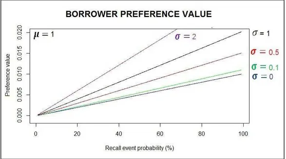
3.2 Borrower’s Preference Value Simulation

We start by analysing the model parameter impacts (𝜇 , loan fee drift (𝜎), loan fee stochastic share; andrecall event at = probability.

The initial loan fee, , was set to 1%, which is reasonable according to our empirical data (Appendix 1). Initial stock price was normalised as = .

In the first graph, we simulated the process without stochastic share, 𝜎 = , with recall probability varying from 1% to 99% among several loan fee drifts, 𝜇 (-1; 0; 0.1; 0.2; 0.5; 1; and 2).

Figure 2. Borrower’s preference value: recall probability variation among several loan fee drifts.

The preference value rises with recall probability and loan fee drift. Since zero or negative drifts reduce the loan fee, a recall event does not concern the borrower, rendering the recall option worthless.

(30)

18

Figure 3. Borrower’s preference value: recall frequency variation, fixed loan fee drift, different loan fee shares.

Loan fee stochastic share also raises the preference value. The next one inverts the first graph, without stochastic share, by varying the loan fee drift among several recall probabilities ( = ; = . ; = . = .9).

Figure 4. Borrower preference value: loan fee drift variation among different recall probabilities.

(31)

19 Finally, we have set a fixed loan fee drift, 𝜇 = , and varied the loan fee stochastic share among several recall event probabilities ( = ; = . ; = . ; =

. = .9).

Figure 5. Borrower preference value: stochastic share variation, fixed loan fee drift, different recall probabilities.

(32)

20

3.3 Lender’s Preference Value

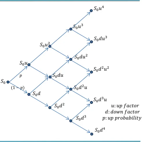
A lender recall option may look like quite similar to a traditional American stock option, whose owner has the right to buy a certain amount of shares for a fixed price at any time until their expiry date. In the recall option, the lender is entitled to recall the loaned shares (at no cost) at any time until the loan expiry date. Therefore, we adapted a binary model, originally proposed for pricing American stock options, to obtain the lender preference value.

One of the simplest, most useful and a very popular technique for valuing an option involves constructing a binomial tree, especially if the option may be exercised at any time until the expiration date.

This American option pricing model proposes a binomial tree which represents different possible paths for stock price over the life of an option. Over each time step, the stock may move up with a certain probability by a certain percentage, or move down by a certain percentage with a certain probability (Hull, J., 2012).

As the time step becomes arbitrarily smaller, this model becomes time-continuous, like the Black-Scholes-Merton model. It can be shown that a European option price given by a binomial tree converges to the Black-Scholes price at the limit, and the only two assumptions required to price an option via a binomial tree are no-arbitrage and risk-neutral valuation (Cox, J.; et al., 1979).

(33)

21 The following diagram illustrates a four steps binomial tree that represents the process followed by a stock price:

Figure 6. Four-step binomial tree stock price process − : : : 𝑦

For solving the American option price, we proceed as follows: at the final node, = , as illustrated above, American and European option prices match its prices; for a call option they value the final stock price minus the strike price, and for a put option they value the strike price minus the final stock price.

At the earlier node, = , as in the example, one can measure the discounted expected future pay-off, after setting the upper node with probability and pay-off as described above, and the lower node likewise. Moving from back-forwards we can set all expected pay-offs and compare them with the given value by immediately executing the option; the greater value establishes the option stop rule.

Our lender preference value framework establishes the following assumptions: . Stock price is driven by a binomial tree process.

. Investors (lenders) are risk-neutral.

(34)

22 . Risk-free interest rate is known and fixed.

As mentioned earlier, the preference value is measured by the difference between lender pay-offs with and without a recall option. The latter must be equal or less than the former. The final pay-off node is set to zero, since the recall option is meaningless at the loan expiration date. Then, we move forwards and compare discounted expected pay-off with immediate pay-off, as in the American option price model. By contrast, in this framework, the lenders balance the earnings from loan fee, , in comparison.

Pay-off without recall option:

Π = − + (eq. 7) Pay-off with recall option:

Π _′ = 𝜏− + _𝜏 < 𝜏 < (eq. 8)

Difference between pay-offs with and without stock recalled at = 𝜏:

Π − Π ′ = 𝜏 − + 𝜏− [ − + ] = 𝜏 − + 𝜏 −

At each node, the lender compares today's with tomorrow's pay-offs:

1. Today: 𝑦 _=𝜏 = 𝜏 − + _𝜏 − − −𝜏 _=𝜏[ ] (eq. 9) 2. Tomorrow: 𝑦 _=𝜏+ = − Δ [ . 𝑦 + − . 𝑦 ₋ ] (eq. 10)

For that node, we set the lender preference value as the maximum pay-off chosen from the greater value above, restricted to positive values, and move back until = .

Model variables:

: Initial stock price. : Final stock price. : Loan number of periods. 𝜏: Stock price at = 𝜏, 𝜏 .

: Loan fee. : risk-free interest rate. Both as continuously compounded.

𝑦 : Future pay-off at upper node.

𝑦 − : Future pay-off at lower node.

(35)

23

3.4 Lender’s Preference Value Simulation

We have simulated the framework above by a numeric exercise after adopting special values for some parameters, and varying other parameters through a large range of values. Some parameters were fixed or normalised as follows: = (therefore, the preference value relative to the stock price is also normalised); =

+ = , meaning the standard loan period. Although not recorded in our dataset, the loan period standardized by the Brazilian Stock Exchange is 34 days: one month (~21 business days) plus 4 days, which is the time length to re-loan the shares and keep the parties involved; and ∆ = 𝑦 = 𝑦 . Finally, the parameters , , and were allowed to vary in order to measure their impacts.

The preference value was set as the option value at time = , after proceeding back-forwardly in a similar way as for the American option using the binomial tree model, as explained above.

Stock price volatility, 𝜎, is a secondary parameter that enters the model in the following analysis.

The first set of parameters was chosen to obtain zero-expected net return, in other words, the asset returns, in probability, the same return as the risk-free interest rate.

To match volatility, we set = 𝜎√∆ and = −𝜎√∆ .

And to match the stock expected return and risk-free rate, we set = ∆𝑇− − , which comes from a risk-neutral expectation.

We then studied the impact of varying the variables risk-free interest tax, loan fee and asset volatility.

(36)

24

Figure 7. Lender’s preference value: expected return, risk-free rate variation among several loan fees.

Both loan fee and risk-free rate, in this case, have no impacts on the preference value.

The next one varies the loan fee between different risk-free interest rates.

Figure 8. Lender’s preference value: expected return, loan fee variation among several risk-free interest rates.

(37)

25

Again, we notice no parameter’s impact. The last one varies stock price volatility within a set of risk-free interest rates and loan fees, but we obtained the same graph for any value of loan fee and risk-free interest rate combination.

Figure 9: Lender’s preference value: expected return, volatility variation

Since we have again found no response, we altered parameter , leading the stock price process probability to move up or move down from zero-expected net return. We set by adding a new parameter, 𝜀, and varied the risk-free interest rate among different 𝜀 values (-0.2; -0.1; -0.05; 0 and +0.05), which increases or reduces the stock expected return as follows:

= ∆𝑇−

− + 𝜀 (eq. 11)

(38)

26 In this case, the preference value responds to the stock expected returns, reaching positive values only for negative expected returns (as for the risk-free interest rate); the lower the expected return, the higher the preference value. Therefore, for every interest rate we adjust the probability, = ∆𝑇₋− , regardless of

𝜀 value, and the preference value does not change with risk-free interest rate variation, loan fee or stock volatility for similar reasons.

In the next set of simulations, we propose parameter combinations so that stock has zero-expected rough return relative to the risk-free interest rate. In the next graph we set the following combinations: = . ; = .99 = . , with risk-free interest rate varying among different loan fees ( = . %; = . %; = % = %).

Figure 11. Lender’s preference value: negative expected return, risk-free rate variation

We notice that, once the stock has a negative expected return, the preference value rises with the risk-free interest rate and lowers with the loan fee.

(39)

27

Figure 12. Lender’s preference value: negative expected return, risk-free rate variation

(40)

28

3.5 Equilibrium Model

Once we have obtained lender and borrower preference values – the reasonable value each investor believes it is worth the recall option (i.e. taking into account that the recall event either reduces or increases the risk), we propose an equilibrium model to price the recall option seen on our empirical results, that is, its market value.

To begin with, let us think hypothetically that the recall option is set by a regulator authority. For example, the recall option is fixed at 30% of the loan fee freely agreed by lender and borrower for a loan contract without recall option. Therefore, for a 10% loan fee without recall option, the same contract would worth 7% with it.

The lender sees the above recall price (30%) as a discount to be given at the loan fee (reward) in order to settle a loan contract with recall option, thus the lender would wish the cheaper price as possible.

On the other hand, the borrower sees such a price as a bonus to be received, which lowers his loan cost, and thus the borrower would wish the highest price as possible.

Therefore, the preference value represents a preference range (a set): the lender accepts any value between zero and LPV to impose the recall option, whereas the borrower accepts any value between BPV and +∞, which is bounded by the loan fee itself, [𝐵 , _ℎ ].

We have then three possibilities: < 𝐵 > 𝐵 𝑦.

In case, < 𝐵 :

From this condition on, lenders and borrowers will establish an equilibrium point to set the market price. The recall price will be as close as possible to LPV or as

close as possible to BPV, depending on each investor’s market power.

(41)

29 Here, 𝜃 represents the lender’s monopoly power, 𝜃 , indicating that the closer to 1 the higher the monopoly market. We could propose 𝜃 as a function from the lender market concentration index, 𝜃 = . Therefore, the recall price would be:

= + 𝐵 − − 𝜃 = 𝜃. + − 𝜃 . 𝐵 (eq. 12)

In case, > 𝐵 :

In this case, the preference sets overlap each other as any value within the range [𝐵 , ] would be accepted by both investors. Knowing that, each investor

will offer a more advantageous value which still would be within the other’s

preference range. This recursive exercise would repeat itself until an equilibrium is reached according to each investor’s market power.

Where 𝜃 is also the lender monopoly power. Therefore the recall price would be:

= 𝐵 + − 𝐵 − 𝜃 = 𝜃. 𝐵 + − 𝜃 . (eq. 13)

(42)

30

4. EMPIRICAL ANALYSIS

4.1 Initial Results

The first empirical analysis performed aimed to study the recall option impacts on the loan fee. We initiated by producing graphs to show the average loan fee in a given period (whether a day, week or month), separated by loan contracts with and without the recall option. Even after weighting the loan fee according to quantity or volume, the average fee for contracts with recall option tended to be higher than those without, which contradicts our prediction. We, therefore, restricted our graph to only one ticker, and after performing it for the 20 most liquid tickers, one by one, we found almost the same pattern, excluding the cross-sectional variance from our rough analysis.

Next, we performed several regression analyses using the recall option as a dummy variable, assuming values one and zero for deals with and without recall option, respectively. All the result coefficients were positive (meaning a higher loan fee for recallable stock), thus reinforcing the conclusion drawn in the graphs. We then restricted the regressions to loan fee percentiles, obtaining either the same or even worthless results for high and low quartiles of loan fees.

By this point we were quite perplexed with the results, and we decided to ask a few routine questions to market dealers in order to see how the Brazilian loan market functions on the trade floor.

One mutual fund operator told us that, as a frequent short-term seller, he does not mind having to pay any loan fee as long as it seems reasonable or even if the loan contract is recallable. However, the recall option becomes of concern when the loan supply shrinks, or in other words, when it is hard to find brokers with stock available for lending.

(43)

31

4.2 Market Concentration Index

In order to present a scarcity situation for borrowers in which a particular stock is hard to find at a reasonable loan price, we have proposed a market concentration index serving as a proxy for search cost, which has been widely discussed in the recent literature.

A common and simple accepted measure for market concentration is the Herfindahl-Hirschman Index.

This index is obtained by summing up the squares of individual market shares of each firm in the industry. The result is a value between zero and one. The closer a market is to being a monopoly, the higher the market's concentration (and the lower its competition). If, for example, there is only one firm in the industry, this firm would have 100% of the market share ( = ), and the HHI value would be 1, indicating a monopoly (it is also common to consider each market share as a percentage, with HHI values ranging from 0 to 10.000). If there are thousands of firms competing, each one would have nearly 0% of the market share, and the HHI would be close to zero, indicating almost perfect competition.

The U.S. Department of Justice considers a market with a result of less than 0.1 to be competitive, whereas that with 0.18 or greater to be a highly concentrated market. As a general rule, mergers and acquisitions increasing the HHI by more than 0.01 point in concentrated markets raise anti-trust concerns.

In order to measure the scarcity in the loan market, we have proposed the use of the Herfindahl-Hirschman Index, as follows:

, = ∑ , , =

, : Herfindahl-Hirschman index for stock (ticker) at time (month or week). , , : market share of lender (or broker) for stock (ticker) at a given time (month or week) in terms of quantity (proportion of the whole quantity).

: number of lenders (or brokers) offering (closed offers considered only) stock (ticker) during a period of time (month or week).

(44)

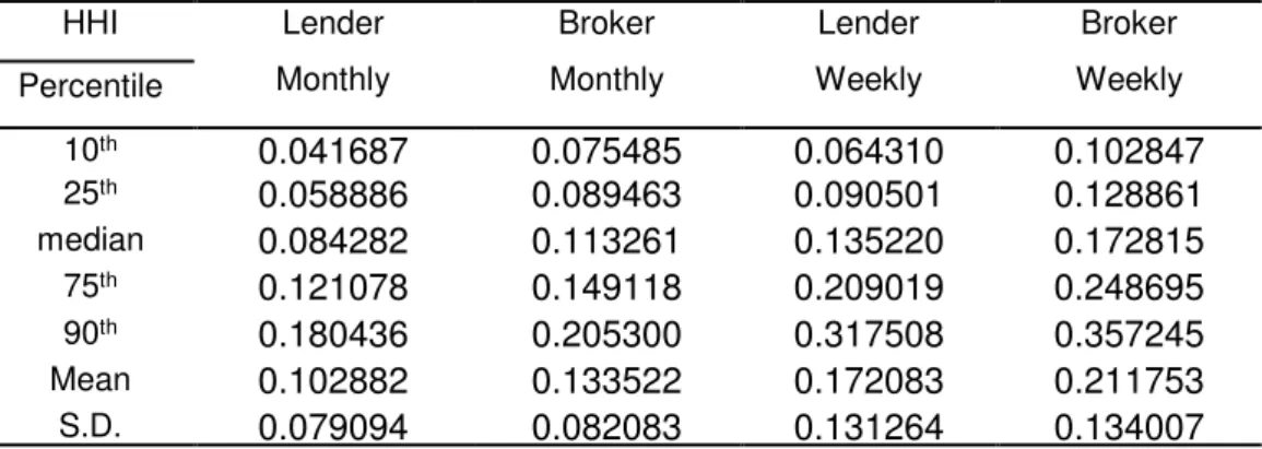
32 The next table summarises some basic statistics for the four different indexes constructed, considering three different liquidity cuts (55, 100, 150).

Table 3. Herfindahl-Hirschman index cross-sectional descriptive statistics in terms of the 55 most liquid tickers.

HHI Lender Monthly Broker Monthly Lender Weekly Broker Weekly Percentile

10th _0.041687 _0.075485 _0.064310 _0.102847

25th _0.058886 _0.089463 _0.090501 _0.128861

median 0.084282 0.113261 0.135220 0.172815 75th _0.121078 _0.149118 _0.209019 _0.248695

90th _0.180436 _0.205300 _0.317508 _0.357245

Mean 0.102882 0.133522 0.172083 0.211753 S.D. 0.079094 0.082083 0.131264 0.134007

10th _0.048958 _0.079199 _0.074145 _0.111299

25th _0.067577 _0.097466 _0.106810 _0.146053

median 0.099186 0.129564 0.168184 0.208466 75th _0.153934 _0.185676 _0.279731 _0.331203

90th _0.248476 _0.310038 _0.463447 _0.537489

Mean 0.135553 0.172499 0.231329 0.277809 S.D. 0.124850 0.137611 0.194928 0.202501

10th _0.054972 _0.084934 _0.083173 _0.120673

25th _0.080596 _0.109910 _0.127213 _0.166270

median 0.131263 0.163832 0.223438 0.270169 75th _0.247591 _0.298822 _0.434279 _0.500370

90th _0.443659 _0.522599 _0.792388 _0.880664

Mean 0.202304 0.244205 0.324269 0.371937 S.D. 0.194574 0.206787 0.268743 0.271288

(45)

33

• All distributions seem to be asymmetric on the left (mean > median).

• Broker deals are more concentrated than the lender ones.

• Weekly aggregations are more concentrated than the monthly ones.

• Bottom (mostly illiquid) shares are more concentrated than the more liquid ones for borrowing.

4.3 Regression Analysis

Once we assembled the four HHI variables, we proposed a way of capturing the interaction between recall option and HHI variables and their loan fee impact. A simple and effective way to do so is to combine the variables by multiplying them. The recall option has value one when it is recallable, whereas HHI has value close to one when the market is highly concentrated. Therefore, the interaction within recallable loans increases as the market concentrates and the option becomes of concern, requiring intuitive direction.

As the HHI concentration indexes are measured for a given period of time (month or week), an observation at the beginning of that period would capture future events via contemporaneous H-H index. Despite this, investors are only able to study past market concentration, which affects the current search cost for a particular stock.

The liquidity filter separates the 55 most frequent tickers accounting for 744,922 observations for monthly aggregation and 761,958 for weekly aggregation on a deal-by-deal basis (i.e. 100 tickers: 904,750 observations for monthly aggregation, and 926,666 for weekly aggregation; 150 tickers: 945,769 and 968,922 observations, respectively). The following equation was performed by using the four HHI variables constructed (monthly and weekly, lender and broker).

The coefficients were estimated by using ordinary least square and its variance-covariance matrix by robust estimation in order to allow variance-covariance between independent variables, as follows:

̂ = ̂ ∑ ̂′_̂

𝑁

=

̂

̂: estimated ordinary variance-covariance matrix.

(46)

34 Equation 14

, ,𝑑 𝑦, = + . , − + . , − . _ 𝑦, ,𝑑 𝑦,

+ . _ 𝑦, , 𝑑 𝑦, + . 𝑦, , 𝑑 𝑦, + 𝑦+

+ 𝜀, ,𝑑 𝑦,

, ,𝑑 𝑦, : loan fee asked by lender , or through broker , for lending stock (ticker) , on business day _𝑦, within deal listed by observation (offer code), which identifies all deals in our data set.

, − : Herfindahl-Hirschman index calculated for stock (ticker) , at the previous period, − (month or week).

_ 𝑦, , 𝑑 𝑦, : recall option dummy (= , if recallable, = , if not); for lender offer, or through broker , for stock (ticker) , on business day _𝑦, within deal listed by observation (offer code).

𝑦, ,𝑑 𝑦, : Loan quantity (number of shares), for lender offer, or through broker , for stock (ticker) , on business day _𝑦, within deal listed by observation

(offer code).

𝑦: Fixed effect for every business day on data set.

: Fixed effect for every stock (ticker) on data cut-off (55, 100 or 150).

𝜀, , 𝑑 𝑦, : regression error.

(47)

35

Table 6. Regression results for Equation 14 in terms of the 55 most liquid stocks. Lender Monthly Broker Monthly Lender Weekly Broker Weekly Lagged HHI ( ) -3.469 -51.000 -1.588 -29.361 -0.658 -19.874 -0.717 -23.853 Lagged HHI*Recall ( ) -3.562 -26.185 -3.481 -28.566 -0.844 -10.677 -1.261 -16.683 Recall dummy ( ) 0.488 33.825 0.580 34.485 0.297 22.530 0.400 25.787 Quantity ( ) 8.25.10-8 _3.525 _7.40.10-8 _3.293 _6.99.10-8 _3.173 _6.91.10-8 _3.148

Constant ( ) 2.184 40.136 2.004 37.229 1.947 36.076 1.958 36.128

Fixed Effectfirm YES YES YES YES

Fixed Effectday YES YES YES YES

R2_(adj.) _0.493988 _0.491534 _0.491187 _0.491607

Obs.: Coefficient estimations on the left and t-statistics on the right within each cell.

Every coefficient turned out to be significant. One may notice that only the recall option points to a coefficient with counter-intuitive direction (positive value), whereas the interaction points to a direction intuitively (negative).

Intuition would suggest that large deals (i.e. involving a large number of shares loaned) come from big investors with extensive market connections and great bargaining power. In the case of short-sellers, these investors may bargain for a reduced loan fee, but in the case of lenders, such investors may bargain for a higher loan fee. This thinking leads to a balance of power within the market. Although significant, the quantity coefficient shows that, on average, quantity barely changes loan fees for contracts lower than 1,000,000 shares, although it does indicate that lenders might have a greater bargaining power than borrowers due to the positive sign.

The lagged HHI alone seems to be counter-intuitive (due to their negative coefficients), indicating that past market concentration accounts for a loan fee reduction. Therefore, we proposed a loan fee dynamics aimed to capture the loan fee increasing. Rapid HHI growth may give investors the impression that the market will soon become scarce, generating concern around recall probability and increasing loan fees. Therefore, we constructed the HHI percentage growth as follows:

∆% = − −

−

(48)

36 Equation 15:

, ,𝑑 𝑦, = + .

, − , −

, − + . , − . _ 𝑦, , 𝑑 𝑦,

+ . _ 𝑦, , 𝑑 𝑦, + . 𝑦, , 𝑑 𝑦, + 𝑦+

+ 𝜀, ,𝑑 𝑦,

We regressed again for the each four HHI variables (monthly and weekly, lender and broker) and obtained the coefficients and t-static estimations shown in the table below:

Table 7. Regression results for Equation 15 in terms of the 55 most liquid stocks. Lender Monthly Broker Monthly Lender Weekly Broker Weekly

− − ⁄ − ) 0.370 67.581 0.400 60.237 0.110 27.688 0.194 30.459

Lagged HHI*Recall ( ) -4.649 -36.755 -3.401 -29.648 -1.057 -14.173 -1.358 -18.793 Recall dummy ( ) 0.578 42.181 0.572 35.711 0.325 25.729 0.417 28.075 Quantity ( ) 4.02.10-8 _1.900 _4.42.10-8 _2.149 _4.85.10-8 _2.286 _3.96.10-8 _1.937

Constant ( ) 1.902 35.297 1.795 33.515 1.843 34.384 1.819 33.648

R2_(adj.) _0.496795 _0.493939 _0.491737 _0.492630

The interactive variable remains significant and intuitive (negative sign). In both equations, the absolute value of the interactive variable coefficient exceeds the coefficient of the recall dummy alone, indicating that recallable loans do indeed accept reduced loan fees. The overall sum demonstrates that the recall option costs from 0 to 4% a year, on average, assuming that the market is highly concentrated. This conclusion may be questioned if one multiplies the interaction variable coefficients by the mean (or median) HHI values. Nonetheless the recall event impacts the loan fee at higher HHI percentiles, probably above the 90th_percentile,

where the coefficient sums are still negative.

Equation 15 points out that such a growth is in line with our previous prediction, showing that as market concentration rises, so does the loan fee.

(49)

37

5. Robustness

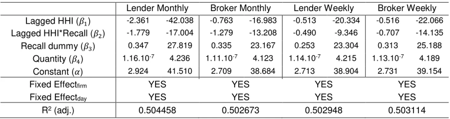
Our first concern about robustness refers to the frequency filter, and thus we applied the 100 and 150 most frequent tickers to Equations14 and 15, respectively.

Equation 14:

, ,𝑑 𝑦, = + . , − + . , − . _ 𝑦, ,𝑑 𝑦,

+ . _ 𝑦, , 𝑑 𝑦, + . 𝑦, , 𝑑 𝑦, + 𝑦+

+ 𝜀, ,𝑑 𝑦,

Table 8. Regression results for Equation 14 in terms of the 100 most liquid stocks. Lender Monthly Broker Monthly Lender Weekly Broker Weekly Lagged HHI ( ) -2.361 -42.038 -0.763 -16.983 -0.513 -20.334 -0.516 -22.066 Lagged HHI*Recall ( ) -1.779 -17.004 -1.279 -13.208 -0.490 -9.346 -0.707 -14.135 Recall dummy ( ) 0.347 27.819 0.335 23.167 0.253 23.304 0.313 25.188 Quantity ( ) 1.16.10-7 _4.236 _1.11.10-7 _4.123 _1.14.10-7 _4.215 _1.13.10-7 _4.189

Constant ( ) 2.924 41.510 2.709 38.684 2.713 38.904 2.731 39.154

R2_(adj.) _0.504458 _0.502673 _0.502948 _0.503114

Table 9. Regression results for Equation 14, in terms of the150 most liquid stocks. Lender Monthly Broker Monthly Lender Weekly Broker Weekly Lagged HHI ( ) -1.935 -41.675 -0.880 -22.779 -0.580 -24.924 -0.595 -27.269 Lagged HHI*Recall ( ) -0.755 -9.741 -0.728 -10.145 -0.212 -4.800 -0.380 -9.053

Recall dummy ( ) 0.259 24.102 0.277 22.747 0.218 21.286 0.259 22.659 Quantity ( ) 1.25.10-7 _4.201 _1.21.10-7 _4.117 _1.22.10-7 _4.148 _1.22.10-7 _4.145

Constant ( ) 2.867 41.445 2.733 39.700 2.726 39.738 2.751 40.106

R2_(adj.) _0.509169 _0.508082 _0.508447 _0.508588

(50)

38 Equation 15:

, ,𝑑 𝑦, = + .

, − , −

, − + . , − . _ 𝑦, , 𝑑 𝑦,

+ . _ 𝑦, , 𝑑 𝑦, + . 𝑦, , 𝑑 𝑦, + 𝑦+

+ 𝜀, ,𝑑 𝑦,

− − ⁄ − ) 0.343 72.304 0.386 66.196 0.101 28.379 0.182 33.110

Constant ( ) 2.585 36.652 2.524 36.055 2.576 37.072 2.576 36.965

R2_(adj.) _0.507524 _0.505258 _0.503386 _0.50405

− − ⁄ − ) 0.322 71.762 0.364 65.867 0.098 28.375 0.179 33.535

Constant ( ) 2.591 37.343 2.538 36.806 2.575 37.603 2.576 37.509

R2_(adj.) _0.511915 _0.510311 _0.508737 _0.509347

Again, we can see the same conclusion as in Equation 14, after comparing the results for Equation 15 applied within the 55 most frequent tickers. The interactive variable remains significant and negative. Its absolute value has also decreased, but it surpasses the recall dummy coefficient.